Aircraft fleet route optimization based on cost and low carbon emission in aviation line alliance network

Abstract

This paper studies the flight path optimization problem of air cargo companies in aviation line alliance. There are two limitations in this paper. One is to limit of the number and location of airbases and capacity in the air network. The other is to limit of flight time and airspace capacity of full cargo aircraft in actual operation. Considering the influence of alliance on operation, the selection probability of air alliance is introduced. It is assuming that all cargo aircraft is one type, the unit transportation cost of every aviation line is the same as each other, the queuing problem of aircraft landing is not considered, and the network transportation demand of itself must be completed by an airline. It proposes a directed aircraft fleet routing problem optimization model (SMDDDAAAFRPTW) with multi-airbase stochastic and time constraints to minimize total operating cost and flight distance. Using the multi-objective optimization algorithm NSGA-II by most scholars, and improving the initial solution generation step, introducing Genetic engineering into cross-mutation to solve the optimal number and location of air bases and fleet routing of multiple aircraft. Comparing with the weighted method and ant colony algorithm, it shows that the improved NSGA-II algorithm is effective and has better computational efficiency. The results show that the more segments are selected for outsourcing, the lowest cost of network and the lowest carbon emission. This kind of decision-making behavior is only suitable for the initial operation phase of the enterprise.

Keywords

Aircraft fleet route optimization multi-airbases stochastic time and capacity constraints improved NSGA-II algorithm

1 Introduction

At present, with the increase of global air cargo demand, the environment also puts forward bigger requirements. China’s low carbon plan proposes to reduce the carbon dioxide emissions of civil aviation units by 11% in 2020. Therefore, under the premise of increasing business demand and air pollution caused by air transport, how to reasonably plan air transport options and fleet routes is an important issue. In this paper, the problem of aircraft fleet route optimization under the airline alliance is studied. Through the airline alliance, the mileage is saved and the number of aircraft usage is reduced, so as to reduce the environmental pollution of air transportation and the business cost of enterprises. At present, there are few researches on the coalition choice of air transportation. Most scholars focus on the impact of the Coalition on customers, the optimization mode of network and the distribution of interests under the coalition. This study is based on the revenue that a cargo airline and other air passenger or cargo companies can obtain according to the transportation choice behavior of different segments under the route alliance to determine the probability of choice behavior.

So the problem of aircraft fleet route optimization with multi-airbases stochastic and time constraints under route alliance can is presented in this manuscript. In this paper, the route alliance is considered to determine the aircraft fleet route optimization problem under self operation selection. Compared with the previous route optimization problem, this paper proposes a new route problem, that is air transportation problem with multiple starting and ending points. It refers to the transportation of each segment as a group of starting and ending points. All requirements are directed. And a new alliance cooperation is introduced to determine the optimal problem. So this paper will perform the following steps. Firstly, the probability function of route alliance selection is introduced. It is assumed that there is only one type of cargo aircraft, the unit transportation cost of each segment is the same, the problem of aircraft landing and queuing is not considered, and the demand of its own network transportation must be completed by one airline. All aircraft can only stay overnight at the base airport, and a double-layer objective optimization model of cost minimization and carbon emission minimization is established. The description of the probability function of route alliance selection is to use the improved prospect theory to analyze the game and determine the transport choice behavior of air freight companies in different segments. Design the adaptive NSGA-II algorithm solution model, and compare with the weighted algorithm, and analyze the case of a domestic air freight company to illustrate the optimal route scheme and route operation selection of the airline.

2 Literature review

(1) Aircraft Fleet Route Literature and Its Limitation

For the research of aircraft fleet route optimization, most scholars have established aircraft fleet route deployment or scheduling model. The main purpose of the study is to minimize the cost, balance the use of aircraft and alleviate congestion.

Evaluation model of route choice. Dipasis B. et al. [1] used a binary logit regression model to determine the choice of routes by the users employing instrument flight rules, was found that operational characteristics, such as distance, commercial flights, and altitudes of the flights are critical.

Mathematical programming model of Cost minimization. Yu Zhuo [2] established aircraft fleet route deployment model with the goal of aircraft use balance and cost minimization, and applied the actual data of airlines to solve the problem, obtained a feasible deployment scheme, which provides decision support for airlines. Feng Xiang et al. [3] solved the problem of inbound flight scheduling under the condition of multiple runways, which required the sum of squares of total flight delay time and total delay cost to be the least. Xu J. et al. [4] quantify the fuel and cost benefits of applying extended formation flight to commercial airline operations.

Mathematical programming model of time minimum. Zhang Wei [5] takes the minimum relative deviation between the actual total flight time and the expected flight time as the objective function to determine the assignment between the aircraft and the flight section on the premise of meeting the aircraft scheduling instructions and the aircraft maintenance plan. Wu Donghua [6] aims to solve the problem of aircraft scheduling with the priority of aircraft flight time balance, aircraft take-off and landing times balance and aircraft waiting time minimum. Wang T.C. et al. [7] established times constraint model to meet both optimal sequence and minimal changes of scheduled time of arrival from estimated time of arrival requirements.

Mathematical programming model of safety factor. Liu Jiapeng et al. [8] considered the safety factor and task completion degree, and applied the weight penalty function to comprehensively consider the influence of various factors to establish the model.

Mathematical programming model of reducing flight delay. Cai K. et al. [9] discusses the problem of alleviating airspace congestion and reducing flight delay simultaneously in air traffic flow management to establish a multi-objective air traffic network flow optimization.

Mathematical programming model of other factors. Wei Xing [10] established a phased aircraft scheduling optimization model. Firstly, the nonlinear model of aircraft integrated scheduling problem is established, and further considering the constraints of aircraft type assignment, route generation and flight restriction, the 0-1 integer optimization model of aircraft integrated scheduling with weekly scheduling period and maintenance opportunity is constructed. Zhong H. et al. [11] established a dual objective integer programming model to solve the problem of flight departure scheduling with partial constraints between adjacent airports. Zhang, Y. et al. [12] based on the route air traffic system model composed of route, waypoint and airport, a route scheduling model is proposed. Under the safety related constraints, such as the capacity of the route and the airport, and the speed of the aircraft, the unit transport flow mechanics model is used to describe the system dynamics. Younghoon C. et al. [13] established a maximum-flight-time-constrained multitrip vehicle routing problem with time windows optimization model by small unmanned aircraft systems. Ho-Huu V et al. [14] present the development of a two-step optimization framework to deal with the design of aircraft departure routes and the allocation of flights to minimize cumulative noise annoyance and fuel burn.

There is less research on the flight route of aircraft in the aviation network such as Vehicle Routing Problems, and there is less research on the service level as the objective function. So the paper will establish flight route of aircraft model to solve the flight route optimization.

(2) Methodology

The solutions to aircraft fleet route optimization problems mainly include accurate algorithms, heuristic algorithms.

Accurate algorithm. Wei Xing [10] adopt branch and bound method to solve Integrated optimization model of aircraft scheduling. Wang Lu et al. [15] study on the accurate algorithm of multi-objective optimization of inbound aircraft scheduling. Zhang y et al. [12] propose Lagrange relaxation method Distributed flight routing and scheduling for air traffic flow management. Zheng Q.M. et al. [16] used a graph model of the airport structure to solve the route segment.

Fuzzy optimization algorithm. Wu Donghua et al. [6] developed fuzzy decision theory based on multi-objective.

Heuristic algorithm. Yu Zhuo and Fan Wei [2] developed flight string generation algorithm airport flight route scheduling optimization management. The papers that are interested in detailed reviews of adaptive genetic algorithm are referred to Liu Jiapeng and Zhang Xuesong [8], Feng Xiang and Yang Hongyu [3], Feng Xinling et al. [17], Li Yaohua and Wang Lei [18], Seongim C. et al. [19]. Most papers putted to use hungarian algorithm [5], particle swarm optimization algorithm [20], tabu search algorithm [11], variable neighborhood search algorithm [21], simulated annealing algorithm [22], separation algorithm [23] to solve aircraft scheduling problem.

Based on previous research, this article will take aviation alliances as a breakthrough, consider alliance selection, cost optimization, and carbon emissions optimization as the basis for decision-making, and improve heuristic solving algorithms to solve problems.

3 Model establishment

In this section, we present the aircraft fleet route optimization model, but needs to be assumed that the demand for all OD demands do not exceed the capacity of one aircraft, the traffic volume response in the flight process, as show in Fig. 1. It is assumed that the aircraft landing takes the same time and staggers the landing time, so there is no queuing problem. Segment capacity and flight time are restricted. Related to the actual flight restrictions, the cargo plane is allowed to fly at most once a day on the same segment. The unit transportation cost of each segment in the transportation process is the same. The unit transportation cost of the aircraft is related to the type of aircraft, assuming that the type of aircraft used is the same. If the segment operation is outsourced, the self operated freight volume of the segment airline is affected by the probability of other airlines flying in the segment.

Fig. 1

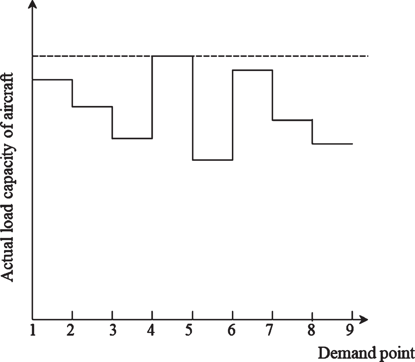
Traffic volume response during aircraft flight.

The problem of aircraft fleet route optimization with multi-airbases stochastic and time constraints under route alliance in the actual problems. The aviation network of airline company has m demand points and multiple alternative aviation bases N. Which the freight demand is D_ij between of each demand points. In the actual flight, the capacity and time constraints on the segment and the capacity constraints of the aviation base are restricted. In addition, airline company adopts alliance each other. When the cost of the segment transportation self operation more than the outsourcing, the segment would take flight outsourcing which demand will be zero. This paper can be regarded as the research on that the optimization problem of aircraft fleet route with time windows and stochastic multiple depots in directed demand and aviation alliance, acroname SMDDDAAAFRPTW, as shown in Fig. 2.

Fig. 2

SMDDDAAAFRPTW problem diagram.

3.1 Problem definition

There are N demand point, the demand and distance of point i to point j are D_ij and d_ij among of them, there are N′ air base. The cost of the airline’s operating process is C_P including the fixed flight cost of the whole cargo aircraft in any segment. The fixed cost is C_FO and unit transportation cost is C_{T
_ij}. C_{W
_ij} represents loading and unloading cost per unit weight. In addition, the takeoff and landing cost of the whole cargo aircraft in any segment is C_PTL[i,j] and each takeoff and landing combined into one and the same. Unit time cost of downtime and waiting is c_w. Unit time penalty cost for early start of service is c_e. Unit time penalty cost of delayed service is c_d.

In addition, the waiting time W_jt of the full cargo t plane for the next segment service at the airport j is related to the total volume of unloading and loading of the aircraft at the airport, among of W_jt equals (D_ijt + D_jit) * ς₁ + ς₂, among of them, ς₁ is loading and unloading time of unit goods, and ς₂ is the fixed value of waiting time, which refers to the maintenance time before the flight of the aircraft. But the cost of waiting at the base airport is not included. Time window of flight allowed in the segment [i, j] is T_[a,b][i,j], the actual starting time $T_{ij}^{t}$ of the full cargo t plane is the sum of the previous takeoff time, the transportation time of the previous segment and the waiting time at the airport. Assuming the average speed of the aircraft is 800 km/h, that is to say $T_{ij}^{t} (2)$ equals $T_{ij}^{t} (1) + \frac{d_{ij} (1)}{800} + W_{jt}$ . The segment of flight time exceeds 24 hours $E_{ij}^{t}$ , obeys the 0-1 distribution, and penalty cost exceeding flight time constraint e. The maximum capacity in the airspace of the segment [i, j] is Q_[i,j]. Airline’s maximum number of aircraft at the airbases n is Q_N. The number of cargo plane is T. Maximum load capacity of the aircraft is Q. On indicators of aviation carbon emissions, γ₁ is the fuel consumption in landing and takeoff stage, which is related to the aircraft type, γ₂ is the fuel consumption per unit time during cruise phase. is the carbon dioxide emission factor of fuel, t_TL is represents the time spent in the landing and takeoff stage. υ is the critical point of self operating probability for alliance.

In the actual operation of one route, airlines can choose alliance self operation or outsourcing according to the freight volume of the segment [i, j]. When airlines choose to join the alliance, the operation choice of different segments is related to their freight volume, freight volume of other cooperative airlines and operation choice of other cooperative airlines. When the airline chooses self operation, the business income is R_{1_ij} = P_x * [t * C_{T
_ij} * d_ij * D_ij - (C_P + C_{T
_ij} * d_ij * D_ij)] + (1 - P_x) * [t * C_{T
_ij} * d_ij * D_ij- $\begin{matrix} (C_{P} + α * C_{T_{ij}} * d_{ij} * D_{ij}) \end{matrix}]$ . When airlines choose outsourcing, the revenue is R_{2_ij} = P_x [A₄ + t * C_{T
_ij} * d_ij * D_ij- $(β * C_{T_{ij}} * d_{ij} * D_{ij})] + (1 - P_{x}) \begin{matrix} A_{8} \end{matrix}$ . Where A₄ and A₈ are the loss value when the airline’s business cannot be carried out normally. Among of them, P_x is the probability of other cooperative alliance companies to choose their own business, D_{1_ij} is point i to point j freight volume of other cooperative Airlines, t is coefficient of return, α is cost sharing coefficient of airline alliance self operation, which 0 < α < 1, β is cost sharing coefficient of airline alliance outsourcing, which β > 1. The probability of airlines choosing alliance self operation is $\frac{R_{1}}{R_{1} + R_{2}}$ , and the probability of alliance outsourcing is $\frac{R_{2}}{R_{1} + R_{2}}$ .

According to the risk aversion problem studied by Rieger, an improved prospect theory of loss value is proposed.

The weight function is used to reflect the degree of risk loss. $π (p) = {\begin{matrix} π^{+} (p) = \frac{p^{ξ}}{{(p^{ξ} + (1 - p)^{ξ})}^{1 / ξ}} \\ π^{-} (p) = \frac{p^{τ}}{{(p^{τ} + (1 - p)^{τ})}^{1 / τ}} \end{matrix}$ (1)

The improved risk-value function is used to describe the risk loss. $v (x) = {\begin{matrix} λ_{1} x, & x \geq 0 \\ - ϑ + ϑ λ_{2} x, & x < 0 \end{matrix}$ (2)

Therefore, the prospect theory function based on the improved risk-value loss is as follows. $V = \sum v (x) π (p)$ (3)

If the decision-maker is more sensitive to the loss, then ϑ > 1. When the loss is not very sensitive, then, ϑ ≤ 1. λ₁ and λ₂ represent the concave and convex degree of the value function in the gain and loss, then 0 < λ₁, λ₂ < 1;p is the probability, ξ and τ represent the change degree of the weight, which also reflects the different attitudes of decision makers towards the gain and risk.

Therefore, A₄ = (- ϑ+ ϑλ₂ * C_W * d_ij * D_ij) * $\frac{((D_{1_{ij}} + D_{ij} - Q) / D_{ij})^{τ}}{{((D_{1_{ij}} + D_{ij} - Q) / D_{ij}^{τ} + (1 - ((D_{1_{ij}} + D_{2} - Q) / D_{ij})^{τ})}^{1 / τ}}$ and A₈ = - ϑ + ϑλ₂ * C_W * d_ij * D_ij.

Among of them, C_W is unit loss cost without carrier. ξ is the change degree of weight when positive income τ is the change degree of weight in case of negative return. ϑ is sensitivity of decision makers. λ₁ is the concave and convex degree of value function in income. λ₂ is the concave convex degree of value function at the time of loss.

3.2 Optimization Model of SMDDDAAAFRPTW

In this paper, multi-objective aircraft fleet route optimization model is established with cost minimization and carbon dioxide emission minimization as objective functions. This problem can be abstracted as a new route optimization problem with time window for multi base random directed demand.

First objective: total cost minimization

The first part is fixed cost, which is the sum of fixed cost of aircraft and fixed cost of base. The second part is the transportation cost, which is obtained by multiplying the driving distance and the unit driving distance rate. The third part is loading and unloading, take-off and landing fees. The fourth part is the cost of waiting, which is obtained by multiplying the waiting time and the unit time rate, and the aircraft waiting at the base does not need to pay the waiting cost. The fifth part is the penalty cost of early service, which is proportional to the time difference. In the sixth part, the penalty cost for delaying service is directly proportional to the time difference. The seventh part is the penalty cost of transportation time, which is caused by the flight start time exceeding 24 hours. The eighth part is the penalty cost of unmanned transportation, that is both sides of the alliance have not allocated transportation capacity to complete the segment transportation.

$\begin{matrix} min Z_{1} = {CF}_{1} + {CF}_{2} + {CF}_{3} + {CF}_{4} + {CF}_{5} \\ + {CF}_{6} + {CF}_{7} + {CF}_{8} \end{matrix}$ (4)

Second objective: carbon emission minimization

According to the International Civil Aviation Organization, the calculation of carbon emissions can be divided into landing and takeoff stage (LTO) and cruise stage [24].

$\begin{matrix} min Z_{2} = \sum_{i = 1, j = 1}^{M} y_{ij} * [γ_{1} * ι + \\ (\frac{d_{ij}}{800} * 60 - t_{TL}) * γ_{2} * ι] \end{matrix}$ (5)

${CF}_{1} = \sum_{t = 1}^{T} C_{P}^{t} + \sum_{n = 1}^{N} {CF}_{O}^{n} * X_{o}$ (6)

$\begin{matrix} {CF}_{2} = \sum_{i = 1, j = 1}^{M} [(α * {CT}_{ij} * d_{ij} * D_{ij} * y_{ij}) \\ + β * {CT}_{ij} * d_{ij} * D_{ij} * (1 - y_{ij}) * P_{x}] \end{matrix}$ (7)

${CF}_{3} = \sum_{i = 1, j = 1}^{M} [({CW}_{ij} * D_{ij} + {CP}_{TL [i, j]}) * y_{ij}]$ (8)

${CF}_{4} = c_{w} * (\sum_{j = 1}^{M} \sum_{t = 1}^{T} W_{jt} - \sum_{o = 1}^{O} \sum_{t = 1}^{T} W_{ot})$ (9)

${CF}_{5} = c_{e} * \sum_{i = 1, j = 1}^{M} \sum_{t = 1}^{T} [max ((a - T_{ij}^{t}), 0)] * y_{ij}]$ (10)

${CF}_{6} = c_{d} * \sum_{i = 1, j = 1}^{M} \sum_{t = 1}^{T} [max ((T_{ij}^{t} - b), 0)] * y_{ij}]$ (11)

${CF}_{7} = \sum_{i = 1, j = 1}^{M} \sum_{t = 1}^{T} E_{ij}^{t} * e$ (12)

$\begin{matrix} {CF}_{8} = \sum_{i = 1, j = 1}^{M} (t * C_{T} + C_{W}) * d_{ij} \\ * D_{ij} * (1 - y_{ij}) * (1 - P_{x}) \end{matrix}$ (13)

$\begin{matrix} s . t . \\ \sum_{i = 1, j = 1}^{M} \sum_{t = 1}^{T} y_{ij} * X_{[i, j]}^{t} * D_{ij} + (1 - y_{ij}) * D_{ij} = D_{ij} \end{matrix}$ (14)

$\sum_{o = 1}^{O} X_{o} = N^{'}$ (15)

$\sum_{i = 1}^{M} X_{[O, i]}^{t} = 1$ (16)

$\sum_{j = 1}^{M} X_{[j, O]}^{t} = 1$ (17)

$\sum_{i = 1}^{M} \sum_{t = 1}^{T} X_{[O, i]}^{t} \leq Q_{N}$ (18)

$\sum_{i = 1}^{M} X_{[i, s]}^{t} - \sum_{j = 1}^{M} X_{[s, j]}^{t} = 0, \forall s \in M$ (19)

$\sum_{i = 1}^{M} \sum_{j = 1}^{M} \sum_{t \in R} X_{[i, j]}^{t} \geq 0$ (20)

$D_{[i, j]}^{t} \leq Q_{[i, j]}$ (21)

$E_{ij}^{t} = {\begin{matrix} 1 \\ 0 \end{matrix}, \begin{matrix} T_{ij}^{t} \geq 24 \\ T_{ij}^{t} < 24 \end{matrix}$ (22)

$y_{ij} = {\begin{matrix} 1 \\ 0 \end{matrix}, \begin{matrix} P_{1} \geq υ, \forall y_{js} = 1 \\ P_{1} < υ \end{matrix}$ (23)

$\sum_{i \in S} \sum_{j \in S} X_{[i, j]}^{T} \leq | S | - 1, \forall t \in R; S \subset V$ (24)

$X_{[i, j]}^{t} \in {0, 1}, \forall i \in V, \forall j \in V, \forall t \in R$ (25)

$X_{o} = {0, 1}$ (26)

Formula (14) indicates that the demand of each segment is met; formula (15) indicates that the number of air bases is limited; formula (16) indicates that all aircraft must start from the air base point; formula (17) indicates that all aircraft must return to the air base point; formula (18) indicates that the aircraft capacity of each base airport is limited; formula (19) indicates that all requirements are met Point service aircraft must leave from this demand point with flow balance constraint; formula (20) indicates that each demand segment can not be serviced; formula (21) indicates that the aircraft’s T carrying capacity in the segment [i, j] does not exceed the aircraft capacity; formula (22) indicates that if the starting flight time exceeds 24 hours, it is counted once, and if it does not exceed 24 hours, it is recorded as 0 times; formula (23) indicates that the segment is or must be completed at that time P₁ ≥ υ. Only the flight can carry out the transportation of the next segment. Select alliance self operation, or alliance outsourcing. Formula (24) (25) (26) is the decision variable, where formula (24) represents the sub path reduction constraint; formula (25) is the decision variable, which indicates whether the segment [i, j] is selected by the aircraft T; formula (26) is whether the point o is the aviation base.

4 Algorithm design

In this paper, the problem of aircraft fleet route optimization is studied, which needs to be solved as follows.

Determine the self operating segment of the alliance.

Determine the number and location of the optimal base of the company.

Flight route of each aircraft.

Because genetic algorithm to solve route assignment problem is used by most scholars, and genetic algorithm is suitable for solving discrete problems. Then the paper select NSGA-II algorithm to solve the aircraft fleet route optimization problem, and the hybrid quantum evolution algorithm is used to solve the directed graph problem of aviation network by matrix coding. The improved NSGA-II algorithm has a relatively strong global search ability, especially when the crossover probability is relatively large, it can generate a large number of new individuals, which improves the global search range. The improved NSGA-II algorithm can improve the rationality of the algorithm The optimization process is shown in Fig. 3.

Fig. 3

Algorithm flow chart.

Step 1: Improve coding form and parameter initialization

Two segment coding form is adopted. The first segment uses chromosome coding, with a total of individuals o, representing alternative aviation bases. The genes on each chromosome represent whether to choose as aviation bases, 1 represents aviation bases, and 0 is not. The second segment uses matrix coding to randomly generate individuals m * m within the feasible region, forming the initial population, in which the previous O individual represents alternative aviation bases. If there are two air bases and 10 demand points, a group of 10*10 will be generated. The numbered of [(1,3), (3,4), (3,4), (4,5), (5,1), (5,1), (2,6), (6,7), (7,8), (8,8, (8,2), (2,1), (1,2), (1,9), (9,10), (9,10),(10,1)] is representing the corresponding solution path, that is three aircraft are needed for transportation, and the service order is route 1 : 1-3-4-5-1, route 2:2-6-7-8-2-1-2, route 3:1-9-10-1.

Step 2: Evaluation of fitness value

According to the aircraft route optimization model, determine the appropriate fitness evaluation function, in this case Fit₁ = Z₁ and Fit₂ = - Z₂. So that the key to the solution lies in the calculation of the probability P₁ of the alliance to select the self-supporting segment, the formation of the path Hamilton circle and the final self-supporting segment under the self-supporting segment.

the probability P₁ that the alliance chooses self operation and determines the self operation segment According to the formula (1) (2) (3), the self selection probability of the alliance among OD demand is calculated. When P₁ ≥ υ, that is recorded as 1, otherwise it is 0, forming a new is matrix A = y_ij[m*m].

Forming the path Hamilton circle under the self-supporting segment

According to the matrix A, several Hamilton cycles are formed and the path is determined. At that time $A = [\begin{matrix} 0 & 0 & 1 \\ 1 & 0 & 1 \\ 1 & 1 & 0 \end{matrix}]$ , it is advisable to $A_{1} = [\begin{matrix} 0 \\ 0 & 1 \\ 1 & 0 \end{matrix}]$ and $A_{2} = [\begin{matrix} 0 & 0 & 1 \\ 1 & 0 & 0 \\ 1 & 0 \end{matrix}]$ , where the marked is the modified submatrix, and the path at this time is 1-2-3-1-3-2-1.

In order to preserve the information of qubit, a new technique of Hamilton circle formation is proposed in this paper. The process is as follows:

The location of the base airport will be determined, and the corresponding rows and columns will be deleted to form a matrix.

If a row with all 0 is found, and the corresponding columns of the row are all 0, then this demand point will be deleted.

The value of diagonal position can only be 0.

If there are more than one 1 in a row of the matrix, take any one as 1, change the other position of the row to 0, and change the other position of the column corresponding to the 1 position to 0.

If there is only one 1 in a row of the matrix, keep it. After traversing all rows, ensure that there is only one 1 in each row.

If there is only one 1 in a column, keep this 1. If there are more than one 1 in a column, randomly select one 1, and move the other 1 to other columns without one. After traversing all columns, ensure that each column has only one 1.

Ensuring that each row and each column have only one 1, forming a sub matrix.

Subtract the submatrix from the matrix to get a new matrix, change all minus one in the matrix to 0, return to step 1, continue to complete the formation of Hamilton circle, until all 1 in the matrix are 0. Then form a group of paths from the first row of the first matrix, and form a chromosome.

Insert the number of the base airport. The first principle is that the time meets the needs. The second principle is that the probability of all bases reaching and transmitting is 1 priority. The third principle is that one base is inserted for every six segments. At insertion, the original segment is repeated and directly the second segment of the next aircraft.

(3) All positions and corresponding segments of 1 are determined as self operation.

(4) calculation of fitness function

According to formula (4) and (5), calculate Fit₁ and Fit₂.

Step 3: Principle of domination

If at least one target of a chromosome p is better than that of the chromosome q, and all targets of the chromosome p are not worse than that of the chromosome q, then the chromosome p dominates the chromosome q, that is p ≥ q, and p₁ > q₁ or p₂ > q₂.

Step 4: Calculate order value By comparing the objective function values of the chromosome p and q, the population ordered was rank_i. If p is dominated q, the order value ratio of p is lower than q. If it is not dominated, it has the same order value. According to the objective function value, select the chromosomes that have not been sequenced, and repeat the process until all the chromosomes in the population are graded.

Step 5: Calculate congestion distance

According to the ascending order of the order values, the target function values are mapped to different edge [-1, 1], and the congestion distance corresponding to the maximum and minimum values of each level is set to inf. For the chromosome not on the edge, the crowding distance is the difference between the two chromosomes, and the crowding distance of chromosome i is calculated according to formula (27) to formula (29).

$crowd_distance 1_{i} = | Fit 1_{i - 1} - Fit 1_{i + 1} |$ (27)

$crowd_distance 2_{i} = | Fit 2_{i - 1} - Fit 2_{i + 1} |$ (28)

$\begin{matrix} crowd_d {istance}_{i} = crowd_distance 1_{i} \\ + crowd_distance 2_{i} \end{matrix}$ (29)

Step 6: Select

According to the calculation results of Step3, Step4 and step5, the tournament method was used to select chromosomes N/2. When rank_i > rank_j, the chromosome j is better than the chromosome i, or when rank_i = rank_j and crowd_distance_i < crowd_distance_j, the chromosome j is better than the chromosome i.

Step 7: Improve crossover, improve variation

According to the crossing probability p_c, using the technology of chromosome recombination and the idea of shear enzyme. First select any segment to cut, and express the cutting site as the cutting gene position, then select any length of the same cutting gene position in other positions of the chromosome to cut, and exchange the positions of the two segments.

Before crossing: 1-4-2-3-1-3-2-4-1-4-3

After crossing: 1-3-2-4-2-3-1-4-1-4-3

According to the mutation probability p_m, it is the same as the improved crossover method. Based on a segment of gene in chromosome, a small segment of gene is selected to mutate. At the same time, after the mutation position, the same gene is selected to connect with the previous segment of gene, and a small segment of gene is mutated with the previous segment of gene.

Before mutation: 1-3-2-3-1-4-2-4-1-4-3

After mutation: 1-4-2-3-1-3-2-4-1-4-3

Step 8: Number of elites

The new population P (t) was formed by combining the chromosomes of parents and children. The next population P (t + 1) was obtained by sequence value, crowding degree and crossing. The chromosomes were selected according to the ascending sequence of fitness value, and finally the chromosomes N were selected.

Step 9: Terminate judgment

When the iterative algebra reaches the expected specification, the program is terminated, and the result is verified. The selected chromosome cannot output the result repeatedly, otherwise, Step2 is returned.

5 Example Analysis

5.1 Parameter setting and basic information

According to the investigation and research of S airline company, The OD matrix of air freight volume of air freight company on a certain day in 2018 is shown in appendix Table A1.

During the actual operation of S airlines, the number of alternative bases is N = 7, The unit transportation cost is 330yuan/ton per 100 km, the maximum carrying capacity of the aircraft is Q = 30 tons, the fixed expenses required for each flight is C_P = 25000 yuan/flight, the handling operation cost is CW = 500 yuan/ton, and the take-off and landing expenses of the aircraft are CP_TL = 20000 yuan/flight. Shenzhen is determined the base of the airline. Other alternative base of the airline sets of the base are Guangzhou, Shanghai, Chengdu, Shenyang, Zhengzhou, Xi’an. In addintion, assuming the construction cost allocated to each day by the aviation base follows the uniform distribution U (3000004000000), the aircraft capacity Q_N of each base follows the linear distribution y = 20 - 2 * x, and suppose the time window of each segment is [U(0,18), U(0,18)+U(2,6)]. Other parameters are shown in Tables 2 and 3.

Table 1
All base of the airline company

Number Determined base city Number Alternative base city

1 Shenzhen 2 Guangzhou

3 Shanghai

4 Chengdu

5 Shenyang

6 Zhengzhou

7 Xi’an

Number	Determined base city	Number	Alternative base city
1	Shenzhen	2	Guangzhou
		3	Shanghai
		4	Chengdu
		5	Shenyang
		6	Zhengzhou
		7	Xi’an

Table 2

Airline alliance operation parameter settings

Parameter index	Specific data
t	2.5
α	0.6
β	1.6
τ	0.9
ϑ	2.5
λ ₂	0.8
C _W	100 yuan / ton per 100 km
P _x	Obey U (0.4, 1)
D _{1_ij}	Obey U (0, 30)

Table 3

Other parameter settings

Parameter index	Specific data
υ	0.5
ς ₁	2000yuan/h
ς ₂	30000 yuan
e	500000 yuan
Q _[i,j]	Obey U [30, 60]
γ₁ [22]	2019.9 kg
ι [22]	3150 g/kg
t_TL [22]	32.9 min
γ₂ [22]	2450 kg/min

5.2 Calculation results

The improved NSGA-II algorithm uses MATLAB R2016b software to run the calculation on the inter core i7-8550u CPU @ 1.80 GHz 1.99 GHz, 8.00GB memory computer.

Determine the initial solution of base of airline is (1,2,3,4,5,6,7), compare the influence of the different parameters for the improved algorithm, such as population size, crossover probability, mutation probability, maximum iteration, as show in Fig. 4. According to the results of Fig. 4, The best parameters of the algorithm are set as follows: population size N = 100, crossover probability pc = 0.8, mutation probability pm = 0.8, maximum iteration MAXGEN = 100. So the optimal results of the number of airports in different bases are shown in Table 4.

Fig. 4

The value of different algorithm parameters.

Table 4

Optimal results of the number of airports in different bases

Scheme	Number of bases base	Site location	Number of aircraft	Total cost Z₁ (10000 yuan)	Carbon emission Z₂ (10000 tons)	Optimal choice
1	2	(1,3)	64	2964	13.86	/
2	2	(1,4)	68	2992	13.71	/
3	3	(1,3,4)	54	2499	11.19	/
4	4	(1,2,3,4)	46	2124	8.91	/
5	5	(1,2,3,4,5)	40	1905	7.46	/
6	6	(1,2,3,4,5,6)	35	1747	6.48	/
7	7	(1,2,3,4,5,6,7)	31	1535	6.07	¡Ì

According to Table 4, when the number of base airports is 7, the carbon emission is the smallest, the cost is also the smallest at this time. Because the more bases there are, the distance required for the aircraft to start from the base and return to the base will be reduced, and the number of aircraft required for route optimization will also be reduced. Optimal route scheme in this case is show in Table 5.

Table 5

Optimal results of the number of airports in different bases

line 1	7-1-5-25-2-11-7	line12	7-4-5-27-5-6-7	line23	7-13-3-14-10-17-7
line2	4-2-3-28-4-31-4	line13	6-21-13-24-17-3-6	line24	1-20-17-19-11-31-1
line3	1-13-6-24-9-20-1	line14	2-19-25-14-30-1-2	line25	6-2-13-2-3-18-6
line4	2-9-14-27-3-19-2	line15	3-3-20-2-23-4-3	line26	7-3-5-14-5-19-7
line5	7-10-30-1-18-2-7	line16	2-2-6-11-13-31-2	line27	1-1-20-31-20-30-1
line6	6-26-2-3-4-6-6	line17	6-1-14-25	line28	3-2-14-2-13-18-3
line7	4-5-10-13-10-14-4	line18	3-19-13-30-1-2-3	line29	3-13-19-20-3-31-3
line8	2-31-3-15-25-19-2	line19	6-1-3-4-3-13-6	line30	4-2-17-2-7-19-4
line9	2-15-20-28-20-27-2	line20	4-25-14-20-5-17-4	line31	7-7-20-25-20-31-7
line10	5-8-30-2-10-2-5	line21	5-31-15-19-14-30-5	——	——
line11	5-3-1-4-20-31-5	line22	4-2-6-2-3-24-4	——	——

5.3 Algorithm comparison

In this paper, two methods are used to compare and analyze the results.

(1) The weighted method is one of the commonly used methods to solve the multi-objective optimization problem. Because the dimensions of the two objectives are inconsistent, the dimensionless standard processing is needed. If $Z_{1}^{*}$ and $Z_{2}^{*}$ are the optimal values of the two objective functions, then the weighted coefficients ω₁ and ω₂ can be used to modify the model.

$\begin{matrix} min ω_{1} \\ \frac{{CF}_{1} + {CF}_{2} + {CF}_{3} + {CF}_{4} + {CF}_{5} + {CF}_{6} + {CF}_{7} + {CF}_{8}}{Z_{1}^{*}} \\ + ω_{2} \frac{\sum_{i = 1, j = 1}^{M} y_{ij} * [γ_{1} * ι + (\frac{d_{ij}}{800} * 60 - t_{TL}) * γ_{2} * ι]}{Z_{2}^{*}} \end{matrix}$ (30)

$\begin{matrix} s . t . \\ ω_{1} + ω_{2} = 1 \end{matrix}$ (31)

$ω_{1}, ω_{2} \geq 0$ (32)

By adjusting the weighting coefficient ω₁ and ω₂, setting the step to 0.05. ω₁ is form 0,0.05,0.1,... to 0.95,1.0, ω₂ is from 1.0,0.95,0.9,... to 0.05, 0, in this time. we can get a set of Pareto optimal solutions, as show in Table 6.

Table 6

Algorithm running time and result comparison

Algorithm	Optimal running time (s)			Calculation results
		Number of bases base	Site location	Number of aircraft	Total cost Z₁ (10000 yuan)	Carbon emission Z₂ (10000 tons)
Improved NSGA-II	55.9	7	(1,2,3,4,5,6,7)	31	1535	6.07
Weighted method	110.5	7	(1,2,3,4,5,6,7)	31	3055	6.07
ACO	69.4	7	(1,2,3,4,5,6,7)	31	1576	6.07

(2) Ant colony algorithm is suitable for searching path problem on graph, but the calculation cost will be large.

The results of the weighted method and ant colony algorithm are consistent with the improved NSGA-II algorithm. The improved NSGA-II algorithm is better than other two methods, whether it’s calculating speed or calculating results, so the improved algorithm is effective and efficient.

5.4 Sensitivity analysis

This section is an analysis of different influencing factors. By analyzing load capacity, fixed cost, cost sharing coefficient, OD demand, the degree of weight in case of negative return, sensitivity of decision makers and coefficient of return, we get the influence of different factors on the optimization result, which has a certain impact on the airline’s decision. And calculate ANOVA through 6 groups of calculation values by improved algorithm.

(1) Restriction of different load capacity Q

When the load capacity constraint Q becomes larger, the unit transportation cost of the aircraft selected on behalf of the airline will become larger. However, the self-supporting segment will be reduced. At this time, the cost and carbon emission under different Q = (30, 35, 40, 45, 50) influences are shown in Fig. 5, and the ANOVA paradigm of load capacity in Table 7. As a whole, with the increase of load capacity Q, the cost is getting lower and lower, and carbon emission is getting lower and lower. It shows that airlines can select the aircraft with more capacity limit in the transportation process. By analyzing the Table 7, it results show that the p-value is small, and the calculation results of the improved algorithm are stable of different load capacity.

Fig. 5

Optimal results under different aircraft capacity constraints.

Table 7

ANOVA paradigm of load capacity

			(a) number of aircraft
	SS	df	MS	F	P-value	F crit
between groups	59.76	4	14.94	20.18919	8.56E-07	2.866081
within groups	14.8	20	0.74
total	74.56	24
			(b) the total cost
	SS	df	MS	F	P-value	F crit
between groups	6322674	4	1580668	23.88837	2.24E-07	2.866081
within groups	1323379	20	66168.94
total	7646053	24
			(c) the carbon emission
	SS	df	MS	F	P-value	F crit
between groups	72362409	4	18090602	2.400891	0.08407	2.866081
within groups	1.51E+08	20	7534953
total	2.23E+08	24

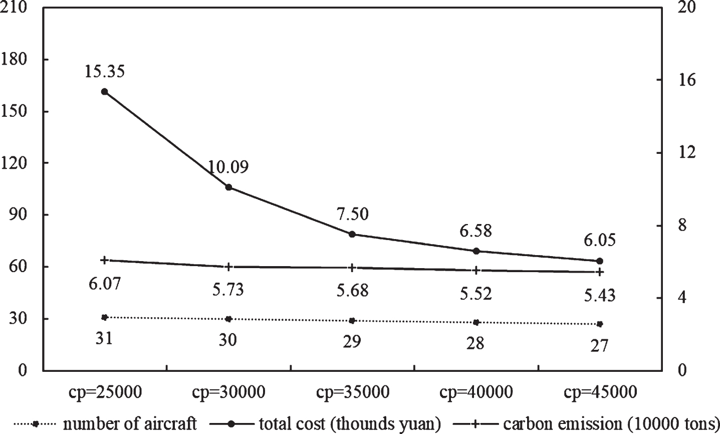
(2) Fixed cost on aircraft C_P

When the fixed cost C_P of aircraft increases, the number of self operating segments will decrease. The cost and carbon emission under different C_P = (25000, 30000, 35000, 40000, 45000) influences are shown in Fig. 6, and the ANOVA paradigm of fixed cost in Table 8. As a whole, with the increase load capacity Q, cost is getting lower and lower, and carbon emission is getting lower and lower. It shows that the fixed cost of airline aircraft greatly affects the optimal result. By analyzing the Table 8, it results show that the p-value is small, and the calculation results of the improved algorithm are stable of different fixed cost.

Fig. 6

Optimal results of different fixed cost.

Table 8

ANOVA paradigm of fixed cost

			(a) number of aircraft
	SS	df	MS	F	P-value	F crit
between groups	1245.36	4	311.34	486.4688	1.29E-19	2.866081
within groups	12.8	20	0.64
total	1258.16	24
			(b) the total cost
	SS	df	MS	F	P-value	F crit
between groups	2.17E+08	4	54197437	1230.942	1.29E-23	2.866081
within groups	880584.8	20	44029.24
total	2.18E+08	24
			(c) the carbon emission
	SS	df	MS	F	P-value	F crit
between groups	17078044	4	4269511	4980.067	1.13E-29	2.866081
within groups	17146.4	20	857.32
total	17095190	24

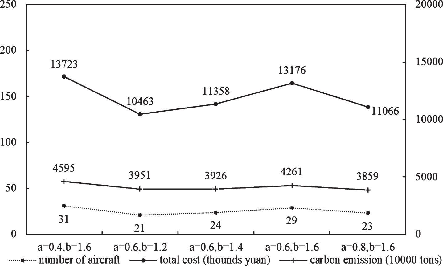
(3) Cost sharing coefficient α, β

When the coefficient of alliance self operation and alliance outsourcing changes, the decision-making of airlines will also change. When comparing and analyzing different values α = 0.4, β = 1.6, α = 0.6, β = 1.2, α = 0.6, β = 1.4, α = 0.6, β = 1.6 and α = 0.8, β = 1.6, the results are shown in Fig. 7, and the ANOVA paradigm of cost sharing coefficient in Table 9. It shows that the larger the cost of self operation α is, the smaller the probability of airlines choosing self operation is, the smaller the total cost is, and the lower the carbon emission is; the smaller the outsourcing cost β is, the smaller the probability of airlines choosing self operation is, the smaller the total cost is, and the lower the carbon emission is. Therefore, airlines should consider both cost and carbon emission in the choice of route transportation behavior. By analyzing the Table 9, it results show that the p-value is small, and the calculation results of the improved algorithm are stable of different cost sharing coefficient.

Fig. 7

Optimal results of different Cost sharing coefficient.

Table 9

ANOVA paradigm of Cost sharing coefficient

			(a) number of aircraft
	SS	df	MS	F	P-value	F crit
between groups	187.36	4	46.84	63.2972973	4.54095E-11	2.866081
within groups	14.8	20	0.74
total	202.16	24
			(b) the total cost
	SS	df	MS	F	P-value	F crit
between groups	34954466	4	8738617	424.7717	4.94E-19	2.866081
within groups	411450	20	20572.5
total	35365916	24
			(c) the carbon emission
	SS	df	MS	F	P-value	F crit
between groups	2712944	4	678236	130.8326	4.86E-14	2.866081
within groups	103680	20	5184
total	2816624	24

(4) the OD demand

The OD demand is the basis of transportation business. When the D = [D, 2D, 3D, 4D, 5D], the compare result is show in Fig. 8, and the ANOVA paradigm of OD demand in Table 10. The result shows that the more OD demand, the more the number of aircraft, the total cost and carbon emission. And when the OD demand multiplied, aircraft is needed more, the total cost and carbon emission is with linear increases. So more and more aircraft is needed to complete transportation business. So the more demand there is, the higher the cost and the smaller the scale effect. By analyzing the Table 9, it results show that the p-value is small, and the calculation results of the improved algorithm are stable of different OD demand.

Fig. 8

Compare results under different OD demand.

Table 10

ANOVA paradigm of OD demand

			(a) number of aircraft
	SS	df	MS	F	P-value	F crit
between groups	4.32E+08	6	72037375	2423.492	4.83E-19	2.915269
within groups	386420	13	29724.62
total	4.33E+08	19
			(b) the total cost
	SS	df	MS	F	P-value	F crit
between groups	9.78E+09	4	2.45E+09	9126.309	2.66E-32	2.866081
within groups	5359799	20	267989.9
total	9.79E+09	24
			(c) the carbon emission
	SS	df	MS	F	P-value	F crit
between groups	1.06E+09	4	2.65E+08	13726.38	4.51E-34	2.866081
within groups	386420	20	19321
total	1.06E+09	24

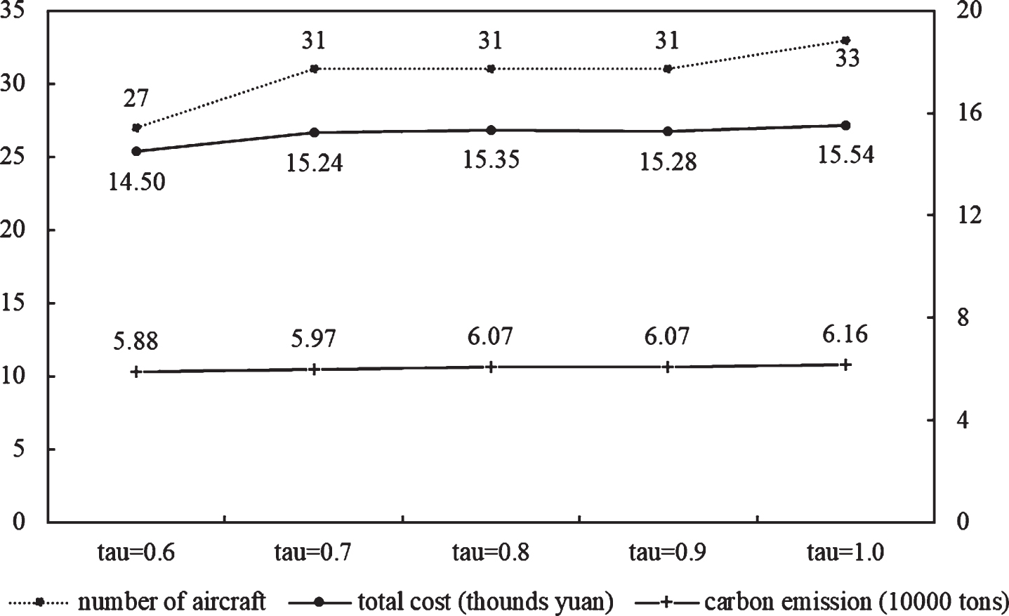
(5) the degree of weight in case of negative return

The weight in case of negative return represents the tolerance of decision makers to risk loss. When the τ = [0.6, 0.7, 0.8, 0.9, 1.0], the compare result is show in Fig. 9, and the ANOVA paradigm of the degree of weight in case of negative return in Table 11. The results show that when the degree of weight in case of negative return increase, number of aircraft, the total cost and carbon emission is increase too. But the growth rate is getting smaller and smaller. The smaller the impact of the degree of weight in case of negative return on the results. By analyzing the Table 11, it results show that the p-value is small, and the calculation results of the improved algorithm are stable of different the degree of weight in case of negative return.

Fig. 9

Compare results under different degree of weight in case of negative return.

Table 11

ANOVA paradigm of different degree of weight in case of negative return

			(a) number of aircraft
	SS	df	MS	F	P-value	F crit
between groups	12.96	4	3.24	2.7	0.060066	2.866081
within groups	24	20	1.2
total	36.96	24
			(b) the total cost
	SS	df	MS	F	P-value	F crit
between groups	2265355	4	566338.7	12.73272	2.6E-05	2.866081
within groups	889580	20	44479
total	3154935	24
			(c) the carbon emission
	SS	df	MS	F	P-value	F crit
between groups	116526.6	4	29131.64	728291	2.56E-51	2.866081
within groups	0.8	20	0.04
total	116527.4	24

(6) sensitivity of decision makers

The sensitivity of decision makers represents the decision makers types. The more sensitive to the loss of decision makers, the more ϑ. When the ϑ = [0.5, 1.0, 1.5, 2.0, 2.5], the compare result is show in Fig. 10, and the ANOVA paradigm of sensitivity of decision makers in Table 12. The results show that when the sensitivity of decision makers increase, the number of aircraft, the total cost and carbon emission is increase too. But the growth rate is getting smaller and smaller. The smaller the impact of sensitivity of decision makers on the results. By analyzing the Table 12, it results show that the p-value is small, and the calculation results of the improved algorithm are stable of different sensitivity of decision makers.

Fig. 10

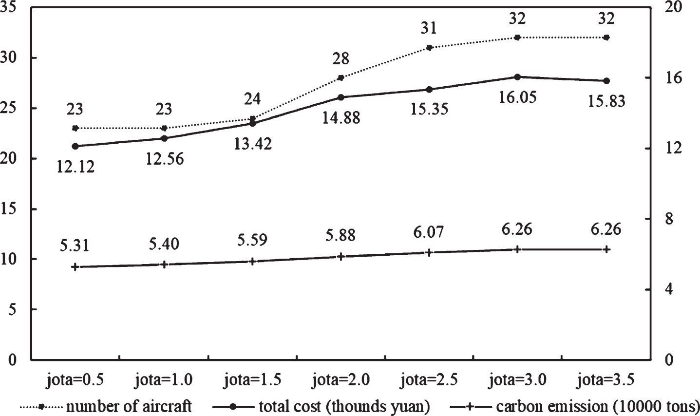
Compare results under different sensitivity of decision makers.

Table 12

ANOVA paradigm of sensitivity of decision makers

			(a) number of aircraft
	SS	df	MS	F	P-value	F crit
between groups	361.5428571	6	60.25714286	66.95238	2.63E-15	2.445259
within groups	25.2	28	0.9
total	386.7428571	34
			(b) the total cost
	SS	df	MS	F	P-value	F crit
between groups	54293198	6	9048866	196.3174	1.52E-21	2.445259
within groups	1290605	28	46093.04
total	55583803	34
			(c) the carbon emission
	SS	df	MS	F	P-value	F crit
between groups	2321138	6	386856.3	13539969	4.01E-89	2.445259
within groups	0.8	28	0.028571
total	2321138	34

(7) coefficient of return

Coefficient of return is the is the ratio of input to output in the process of airline operation. The more coefficient of return means the more profit. When the t = [1.5, 2.0, 2.5, 3.0, 3.5], the compare result is show in Fig. 11, and the ANOVA paradigm of coefficient of return in Table 13. The results show that when the coefficient of return is doubled, the cost is more than twice, and most of them adopt the self operating mode. By analyzing the Table 12, it results show that the p-value is small, and the calculation results of the improved algorithm are stable of different coefficient of return.

Fig. 11

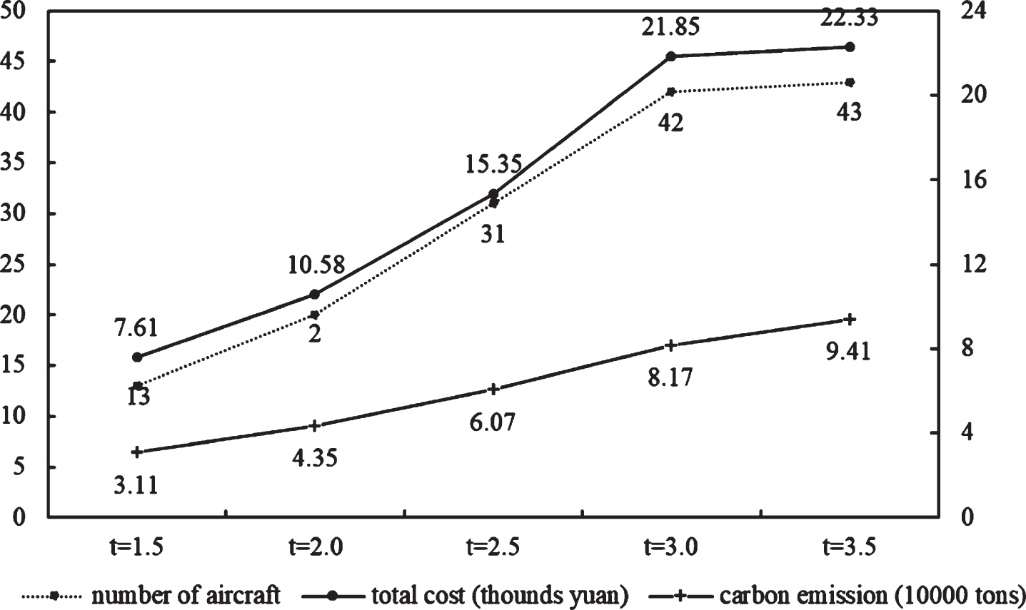
Compare results under different coefficient of return.

Table 13

ANOVA paradigm of coefficient of return

			(a) number of aircraft
	SS	df	MS	F	P-value	F crit
between groups	3636.16	4	909.04	967.0638	1.42E-22	2.866081
within groups	18.8	20	0.94
total	3654.96	24
			(b) the total cost
	SS	df	MS	F	P-value	F crit
between groups	6.66E+08	4	1.67E+08	2704.847	5.02E-27	2.866081
within groups	1231165	20	61558.24
total	6.67E+08	24
			(c) the carbon emission
	SS	df	MS	F	P-value	F crit
between groups	2.19E+08	4	54734188	2.524435	0.073105	2.866081
within groups	4.34E+08	20	21681759
total	6.53E+08	24

6 Conclusion

This paper studies the problem of aircraft route optimization under the air alliance network, introducing alliance transportation selection behavior probability function. The aircraft route is a directed graph optimization problem, which establishes a 0-1 integer programming model to minimize the total cost and carbon emission. Firstly, the probability of self-supporting transportation is calculated by using the improved prospect theory, and the segment of self-supporting transportation is preliminarily determined. By using the improved NSGA-II algorithm, the final self-supporting transport segment and route are calculated.

Therefore, through the research of this paper, the following conclusions are drawn.

Aviation alliance effectively solves the problem of high cost and high carbon emission of airlines. Through aviation alliances outsource small-demand operations, it can reduce waste of transportation resources and costs. By outsourcing business, this part of the business will be merged with other airline business, and carbon emissions will also be reduced.

By comparing the improved algorithm NSGA-II with the weighted method and ant colony algorithm, it shows that the improved algorithm is better than the weighted method and ant colony algorithm in calculation efficiency and results.

Airlines in different aircraft capacity limits, aircraft fixed cost, cost sharing coefficient, penalty cost, will have a certain impact on the choice of aircraft route and cost.

With the increase of load capacity and fixed cost on aircraft, the more outsourcing business, cost is getting lower and lower, carbon emission level is getting lower and lower. The larger the cost of self operation, the lower the total cost and carbon emission; the smaller the outsourcing cost, the smaller the total cost, and the lower the service level.

With the increase of OD demand, the degree of weight in case of negative return, sensitivity of decision makers and coefficient of return, the larger the total cost, and the higher the service level.

Footnotes

Appendix

Table A1

OD matrix of air freight volume (unit: kg)

O\D	Shenzhen	Guangzhou	Shanghai	Chengdu	Shenyang	Zhengzhou	Xi’an	Beijing	Tianjin	Chongqing
Shenzhen	0	4978	1980	2020	1840	0	3654	5200	5953	550
Guangzhou	4700	0	3773	2915	2507	728	2903	8707	0	2574
Shanghai	3518	3173	0	12697	6815	0	5960	14175	6620	0
Chengdu	1878	2066	2165	0	1160	687	971	4453	4750	905
Shenyang	612	1713	2193	1344	0	457	774	2823	1962	1120
Zhengzhou	0	491	0	2555	1771	0	1415	2768	2365	0
Xi’an	2303	2156	3979	1157	1171	1174	0	7207	3854	1298
Beijing	6219	2896	5857	14490	0	1206	7121	0	4363	2295
Tianjin	5532	0	3542	5556	2817	2870	5727	23077	0	8252
Chongqing	2264	576	0	5020	1517	0	1845	1908	2540	0
Nanjing	1040	2183	433	2832	1061	0	0	332	1472	194
Wuhan	0	2134	1957	3007	1048	0	1043	5314	3845	301
ShiJia zhuang	1775	5	620	1882	0	0	1615	0	2651	61
Taiyuan	846	921	1243	0	393	73	783	2733	1673	858
Dalian	0	847	1661	747	0	431	618	0	939	769
Changchun	303	30	971	109	215	162	0	423	843	793
Harbin	1620	1129	2342	568	0	351	775	5074	1175	708
Hohhot	104	783	2041	499	0	369	313	1899	1574	1226
Ji’nan	270	657	1083	753	0	279	439	4698	887	475
Qingdao	285	558	618	259	0	0	0	616	323	330
Hefei	1080	3476	404	2984	1048	0	1160	0	4485	0
Hangzhou	1900	3325	4793	2330	2159	434	2454	733	5934	3863
Ningbo	214	381	0	1620	867	0	861	1301	2131	0
Wenzhou	546	2546	0	368	244	0	152	559	9	0
Fuzhou	1060	3860	0	2162	447	0	1383	3980	2053	0
Xiamen	630	515	1978	356	386	388	546	1938	59	0
Changsha	5031	16	1535	4676	2714	849	2779	5495	0	6162
Nanning	291	260	421	293	112	0	49	855	325	452
Guilin	495	0	405	122	0	0	90	642	0	631
Nanchang	0	72	408	888	189	0	431	2681	406	0
Guiyang	404	750	862	419	82	198	305	1360	1830	0
Kunming	784	1968	1770	1234	395	63	302	1363	0	924
Lhasa	98	0	0	4306	0	0	0	0	0	0
Haikou	200	0	0	491	347	0	2105	460	711	161
Lanzhou	505	457	1951	782	268	101	1254	1459	1000	422
Yinchuan	218	193	596	356	105	72	634	1326	603	284
Xining	218	320	330	296	0	115	469	993	881	1161
Urumchi	1590	984	3496	1396	0	133	2885	3538	1657	1727
O\D	Nanjing	Wuhan	Shijiazhuang	Taiyuan	Dalian	Changchun	Harbin	Hohhot	Ji’nan	Qingdao
Shenzhen	224	0	475	1681	0	540	0	485	564	396
Guangzhou	1578	5245	1612	954	1010	3498	704	1527	1909	2574
Shanghai	1754	3241	1500	5631	1264	4951	2183	4804	4257	847
Chengdu	2267	2623	1297	0	834	1091	397	809	965	133
Shenyang	1011	512	0	629	411	1534	0	0	0	713
Zhengzhou	0	0	0	1552	1648	897	605	791	730	374
Xi’an	0	1113	681	1096	482	0	220	646	660	1104
Beijing	0	5863	0	5942	0	259	3885	6134	5062	3878
Tianjin	5321	4735	9006	2802	2303	2587	1799	3920	2423	1638
Chongqing	2489	1831	418	1018	657	2258	277	4369	2552	1867
Nanjing	0	0	0	1014	0	0	439	843	703	938
Wuhan	0	0	279	1947	0	402	384	562	511	468
ShiJia zhuang	0	771	0	1067	0	0	946	610	303	0
Taiyuan	315	569	225	0	88	149	0	277	206	209
Dalian	0	0	0	148	0	0	0	0	0	0
Changchun	0	206	145	189	0	0	74	119	99	36
Harbin	935	1282	494	273	382	838	0	0	0	177
Hohhot	330	174	431	300	299	203	0	0	0	421
Ji’nan	534	238	545	225	237	345	0	0	0	434

O\D	Nanjing	Wuhan	Shijiazhuang	Taiyuan	Dalian	Changchun	Harbin	Hohhot	Ji’nan	Qingdao
Qingdao	179	375	0	54	0	0	0	77	133	0
Hefei	0	1264	0	1068	0	0	182	652	903	361
Hangzhou	10	1875	0	1313	0	762	1162	1808	1052	1342
Ningbo	0	0	234	1340	758	139	132	0	394	239
Wenzhou	652	612	86	60	87	200	69	206	0	66
Fuzhou	2233	1257	532	948	149	611	318	124	361	0
Xiamen	908	584	502	632	47	483	27	142	326	18
Changsha	1717	3237	1352	716	1057	1351	1133	1924	1083	271
Nanning	338	230	98	342	0	98	57	79	84	0
Guilin	0	0	0	0	0	0	0	0	0	0
Nanchang	571	0	254	1964	0	202	78	149	194	122
Guiyang	469	376	0	0	87	107	48	78	61	0
Kunming	404	826	584	1004	427	596	68	167	347	0
Lhasa	0	0	0	84	0	0	0	0	0	0
Haikou	0	127	0	474	11	483	0	0	0	0
Lanzhou	359	464	152	180	99	273	55	66	52	183
Yinchuan	73	108	0	120	0	55	0	0	61	0
Xining	277	185	0	193	0	0	0	0	0	0
Urumchi	661	1750	426	222	137	132	79	0	0	0
O\D	Hefei	Hangzhou	Ningbo	Wenzhou	Fuzhou	Xiamen	Changsha	Nanning	Guilin	Nanchang
Shenzhen	1932	1040	751	210	194	2708	2523	1080	107	0
Guangzhou	1405	6484	2018	5114	2519	511	428	335	0	119
Shanghai	764	1521	0	0	0	750	1546	2939	1075	1447
Chengdu	2203	1359	583	377	359	618	707	985	148	1187
Shenyang	914	1103	414	424	237	462	269	647	0	521
Zhengzhou	0	94	0	0	0	285	106	1238	699	0
Xi’an	1166	901	1256	442	279	814	683	558	353	1687
Beijing	0	2600	1698	625	346	2777	5602	2163	473	3822
Tianjin	9332	6347	3415	1362	828	1130	0	132	0	1481
Chongqing	0	3488	0	0	0	0	536	20	745	0
Nanjing	0	60	0	0	0	200	411	805	353	0
Wuhan	1373	1153	0	322	284	1634	2136	900	0	0
ShiJia zhuang	0	0	0	0	0	0	536	284	0	0
Taiyuan	600	495	178	201	39	234	231	616	0	357
Dalian	0	0	0	0	0	196	243	287	0	163
Changchun	0	104	101	43	0	194	248	40	0	168
Harbin	865	979	49	24	0	63	534	270	0	183
Hohhot	669	1521	493	0	0	0	261	182	0	147
Ji’nan	578	1306	105	116	72	134	161	211	0	165
Qingdao	89	645	90	0	0	0	190	0	0	0
Hefei	0	0	0	0	0	790	808	881	208	363
Hangzhou	0	0	1426	1154	1067	1105	1561	834	215	1253
Ningbo	0	43	0	0	0	0	124	348	104	0
Wenzhou	0	216	0	0	0	0	200	2	0	9
Fuzhou	285	1834	0	0	0	0	0	409	0	0
Xiamen	311	547	0	0	0	0	0	363	6	0
Changsha	2049	1667	3013	438	0	0	0	1114	467	0
Nanning	290	193	185	95	0	197	117	0	0	1687
Guilin	0	117	66	0	0	0	123	0	0	0
Nanchang	282	486	0	0	0	0	130	229	28	0
Guiyang	291	257	171	0	79	261	218	0	0	291
Kunming	298	480	246	430	774	658	0	529	0	0
Lhasa	0	0	0	0	0	0	0	0	0	0
Haikou	147	0	0	0	0	52	299	0	0	378
Lanzhou	124	367	401	73	160	206	435	0	0	216
Yinchuan	165	77	49	0	0	0	146	0	0	65
Xining	326	0	0	0	0	0	0	0	0	0
Urumchi	1249	124	535	0	0	138	86	0	0	120

O\D	Guiyang	Kunming	Lhasa	Haikou	Lanzhou	Yinchuan	Xining	Urumchi
Shenzhen	816	2747	218	392	321	279	306	612
Guangzhou	3334	4916	765	740	554	1505	618	3361
Shanghai	4166	3074	598	472	1352	1684	456	1803
Chengdu	641	2494	5450	194	797	506	311	1619
Shenyang	547	501	115	175	257	445	99	450
Zhengzhou	1543	717	245	355	365	564	570	635
Xi’an	1108	1028	363	944	3978	1730	1612	1104
Beijing	2897	2284	78	707	1776	2623	1393	2720
Tianjin	4771	5136	988	891	1174	1063	815	993
Chongqing	206	1916	832	202	251	913	157	839
Nanjing	1147	621	0	227	1038	707	0	1043
Wuhan	797	2002	225	305	228	274	287	503
ShiJia zhuang	138	257	0	60	165	46	47	338
Taiyuan	0	894	112	101	212	343	65	212
Dalian	0	287	0	0	84	0	0	0
Changchun	87	0	0	45	152	76	51	187
Harbin	175	265	0	84	23	88	5	34
Hohhot	150	116	0	132	12	0	0	373
Ji’nan	145	410	0	48	103	93	0	181
Qingdao	0	48	0	90	0	0	0	80
Hefei	726	1132	0	530	550	486	117	455
Hangzhou	1260	1160	0	778	488	557	288	1114
Ningbo	236	1400	0	64	524	49	0	373
Wenzhou	0	94	0	4	0	0	36	0
Fuzhou	675	1217	0	233	256	0	108	903
Xiamen	91	229	185	23	312	106	63	277
Changsha	1885	976	0	589	612	492	138	1093
Nanning	0	0	0	201	65	0	0	0
Guilin	0	0	0	82	0	0	0	0
Nanchang	69	1104	0	93	245	58	0	152
Guiyang	0	0	0	103	515	0	0	265
Kunming	1737	509	139	372	139	129	0	100
Lhasa	0	0	0	0	0	0	0	0
Haikou	811	0	0	0	0	0	0	0
Lanzhou	197	193	6	81	0	0	0	488
Yinchuan	0	111	0	0	0	0	0	0
Xining	0	134	177	90	0	0	0	135
Urumchi	71	145	0	45	1572	56	84	0

References

Dipasis

, Brendan

, Choice of route networks: A qualitative model for overland and overwater routes[J], Journal of Aircraft 45(1) (2016), 56–63.

Zhuo

, Wei

, Simulation Research on airport flight route scheduling optimization management [J], Computer Simulation 35(07) (2018), 54–58.

Xiang

, Hongyu

, Improved NSGA-II algorithm for inbound aircraft scheduling [J], Journal of University of Electronic Science and technology 43(01) (2014), 66–70.

, Ning

, Bower

, Aircraft route optimization for formation flight[J], Journal of Aircraft 51(2) (2014), 490–501.

Wei

, Research on Optimization Algorithm for aircraft scheduling problem [D], Tianjin University (2012).

Donghua

, Hongshan

, Yongjun

, Fuzzy optimization algorithm of multi-objective aircraft route allocation model [J], System Engineering Theory and Practice 34(04) (2014), 1011–1017.

Wang

T.C.

, Li

Y.J.

, Optimal scheduling and speed adjustment in en route sector for arriving airplanes[J], Journal of Aircraft 48(2) (2011), 673–682.

Jiapeng

, Xuesong

, Route planning method of special aircraft based on improved adaptive genetic algorithm [J], Journal of Chinese Academy of Electronic Sciences 9(05) (2014), 526–530.

Cai

, Zhang

, m, Xiao, et al., Simulated optimization of aerospace conference and flight delay in air traffic network flow management [J], IEEE Transactions on Intelligent Transportation Systems 18(11) (2017), 3072–3082.

10.

Xing

, Integrated optimization model and algorithm of aircraft scheduling [D], Nanjing University of Aeronautics and Astronautics (2012).

11.

Zhong

, Guan

, Zhang

, et al., A bi objective integer programming model for partially restricted flight department scheduling [J], PLoS One 13(5) (2018), e196146.

12.

Zhang

, Su

, Li

, et al., Distributed flight routing and scheduling for air traffic flow management [J], IEEE Transactions on Intelligent Transportation Systems 18(10) (2017), 2681–2692.

13.

Younghoon

, Bradford

, Youngjun

, A multi-trip vehicle routing problem for small unmanned aircraft systems-based urban delivery [J], Journal of Aircraft 56(6) (2019), 2309–2323.

14.

Ho-Huu

, Hartjes

, Visser

H.G.

, et al., An optimization framework for route design and allocation of aircraft to multiple departure routes[J], Transportation Research Part D Transport and Environment (2019), 76. DOI: 10.1016/j.trd.2019.10.003

15.

, Xiaoning

, Qihuang

, et al., Study on the accurate algorithm of multi-objective optimization of inbound aircraft scheduling [J], Aviation Computing Technology 46(06) (2016), 12–15.

16.

Zheng

Q.M.

, Yiyuan

J.Z.

, Systematic procedure for taxi-route conformance monitoring[J], Journal of Aircraft 49(6) (2012), 1953–1964.

17.

Xinling

, Yuejiao

, Yingxia

, et al., Optimization of flight planning by genetic algorithm [J], Computer Engineering and Design 30(19) (2009), 4468–4471.

18.

Yaohua

, Lei

, Research on aircraft scheduling optimization method based on improved genetic algorithm [J], Journal of System Simulation 28(3) (2016), 620–626.

19.

Seongim

, Daniel

G.M.

, John

E.R.

, Design of an optimal route structure using heuristics-based stochastic schedulers [J], Journal of Aircraft 52(3) (2015), 765–777.

20.

Haibo

, Research and implementation of aircraft scheduling algorithm [D], Nanjing University of Aeronautics and Astronautics, (2007).

21.

Ruyu

, Research on model and algorithm of aircraft scheduling problem [D], Beijing Jiaotong University (2018).

22.

Hong

, Aircraft scheduling problem of airlines: model and algorithm research [D], Southwest Jiaotong University (2003).

23.

Emre

, Çetek

, Point merge concept for en route air traffic flow management[J], Journal of Aircraft 55(6) (2018), 2203–2216.

24.

Peng

, Study on CO2 standard and its impact[D], Civil Aviation University of China (2014).