Continual learning classification method for time-varying data space based on artificial immune system

Abstract

Classification methods play an important role in many fields. However, they cannot effectively classify the samples from sample spaces that are varying with time, for they lack continual learning ability. A continual learning classification method for time-varying data space based on artificial immune system, CLCMTVD, is proposed. It is inspired by the intelligent mechanism that memory cells of the biological immune system can recognize and eliminate previous invaders when they attack again very fast and more efficiently, and these memory cells can evolve with the evolution of previous invaders. Memory cells were continuously updated by learning testing data during the testing stage, thus realize the self-improvement of classification performance. CLCMTVD changes a linearly inseparable spatial problem into many classification problems of several different times, and it degenerates into a common supervised learning classification method when all data independent of time. To assess the performance and possible advantages of CLCMTVD, the experiments on well-known datasets from UCI repository, synthetic data and XJTU-SY rolling element bearing accelerated life test datasets were performed. Results show that CLCMTVD has better classification performance for time-invariant data, and outperforms the other methods for time-varying data space.

Keywords

Artificial immune system classification continual learning machine learning time-varying data

1 Introduction

Machine learning has made remarkable progress over the past two decades in the field of medical [38], industrial produce [32], social life [42], systems and control engineering [29 , 43], equipment fault diagnosis [20 , 44] and national security [24]. Supervised learning classification methods, such as Bayesian networks (BN) [1, 34], k-nearest neighbors (kNN) [28], artificial neural networks (ANN) [23, 30], support vector machine (SVM) [13, 15] and deep learning (DL) [41], play an important role in the field of machine learning. The supervised learning classification method generally uses labeled training data to build a classification model, also referred to as classifier, between data and labels. The classification model is used to classify unlabeled testing data in one of the known classes [3].

Abundant results on supervised learning classification methods were achieved in improving classification accuracy, enhancing classification efficiency, increasing the capacity of dealing with big data, and widening the practice range [17]. However, these research achievements are mainly for the data which is generally an independent of time, and little attention has been paid to the classification method for time-varying data space [4, 40]. In fact, the time-varying data space is frequently observed in the scientific research and engineering fields. But these classification methods cannot effectively classify time-varying data space, and this is illustrated in Fig. 1. There are 3 types of samples, and the sample spaces at t₁ and t₂ time are shown as in Fig. 1a and 1b respectively. The classification model trained by partial of these samples at t₁ time has better classification performance for some time. However, its classification performance gets worse over time. For instance, it cannot effectively classify the samples which are generated between t₁ and t₂ time.

Fig. 1

Sample spaces at different times.

To periodically retrain the classification model based on the newest data or to generate a function between old data and new data are general ways to keep classification performance. A moving-window neural network classification algorithm is proposed to classify the time-varying data [39]. The result of a two-dimensional synthetic experiment shows that it has higher accuracy compared with existing neural network classification algorithms. However, its classification performance was not validated in high-dimensional time-varying data. A process support vector machine model (PSVM) expands the information processing mechanism of the traditional SVM to the time domain [33]. The input of PSVM is a time-varying function. It has a good practical effect on pattern classification problems of time-varying signals. However, how to choose the kernel function of the PSVM is difficult. A new class of probabilistic neural networks (PNNs) [22] and a new time-varying long term synaptic efficacy function-based leaky-integrate-and-fire neuRON model [2] is proposed to work in nonstationary environment. They generate a function between old data and new data, thus making the new data apply to the classification model, but it is difficult to generate the correct function in general.

The image representation of time-series signals in the BoF framework treats a time-series classification problem as a texture recognition task [26]. Experimental results on the UCI time-series classification show that it has higher accuracy. A numerically efficient adaptive sensor fault diagnosis method based on reconstruction-based contributions for continuous time-varying processes is proposed [21]. It guarantees a correct diagnosis of single sensor faults with large magnitudes. A real-time engine load classification from sensed signals can be implemented for the same type of engine with different numbers of cylinders [35]. It was verified by five classes of engine load in the V12 marine diesel engine and has higher accuracy. A classification method of univariate time series based on the framework of information geometry is proposed [14]. It is to project the data from manifold to tangent space. It achieves better performance on a synthetic data and a set of benchmark data sets. An edge computing-based method for real-time fault diagnosis and dynamic control of rotating machines is proposed [12]. It processes sensor data in real time and thus shows potential applications in the rotating machines where fault diagnosis and dynamic control are highly time sensitive. A hybrid method combining the extended Kalman filter (EKF) with cost-sensitive dissimilar ELM (CS-D-ELM) is proposed [19]. The raw data are preprocessed by EKF to produce inputs for the CS-D-ELM classifier. Experimental results show that it is more suitable for real-time fault diagnosis. A recursive variant of the Parzen kernel density estimator to track changes of dynamic density over data streams in a nonstationary environment is proposed [27]. It has low computational complexity, and can efficiently tracking nonstationary probability density. However, these methods have more parameters need to be set.

Therefore, to carry out continual learning classification method research is another way to solve this problem [11]. The classification model can be improved by continual learning the testing samples during the testing stage, which ensures it to keep better classification performance.

The biological immune system is a very complexity and continual learning system. There are many artificial immune algorithms are inspired by its various intelligent mechanisms, such as negative selection algorithm, artificial immune network algorithm, and clone selection algorithm [6 , 25].

This paper proposed a continual learning classification method for time-varying data space based on artificial immune system, CLCMTVD, which is inspired by intelligent mechanism that memory cells of the biological immune system can recognize and eliminate previous invaders when they attack again very fast and more efficiently, and these memory cells can evolve with the evolution of previous invaders. Memory cells were continuously updated by learning testing data during the testing stage, thus realize the self-improvement of classification performance.

The rest of the article is structured as follows. Section 2 is the model of the proposed method. An extensive experimental evaluation of our approach is provided in Section 3. This paper is concluded in Section 4.

2 Continual learning classification method for time-varying data based on artificial immune system (CLCMTVD)

When invaders first attack cells, many appropriate antibodies can be generated by the immune system. After clearing the invaders, appropriate memory cells are born. When the invaders attack again, they can be eliminated very fast and more efficiently [7, 16]. Memory cells can evolve with the evolution of previous invaders. Memory cells were continuously updated by learning testing data during the testing stage, thus realize the self-improvement of classification performance.

The body is like a state space, and the memory cells are used as a classifier, and this classifier can improve itself in real-time according to different invaders.

2.1 Definitions

In order to understand this method better, some concepts used throughout the rest of this paper are defined as follows:

(1) Antibody: A feature vector coupled with its sampling time and associated type. It is used to activate a cell and culture appropriate memory cells. Training samples are used as antibodies in this method.

(2) Antigen: It is the same in representation as an antibody. It is used to attack the immune system. Testing samples are used as antigens in this method.

(3) Cell: It is the basic element of body, store related information, and has a certain shape and size.

There are many ways to describe a cell and a cube or square is used as a cell in this paper. For it is easy to describe the cell division; the cube or square with different sizes could be viewed as the cell with different passages. In other words, the cells with the same passage have the same size.

(4) Cell division: The process of a cell divides into more daughter cells under the cell division strategy. A square cell can divide into 2² daughter cells and a cube cell can divide into 2³ daughter cells in this method.

(5) Passage number (p): The number of times a cell divides. The passage of the initial cell is 0 in this method. The small p value indicates high passage.

(6) Passage of memory cell (pm): This is one of two parameters that need to set in this method. This value is used to ensure every memory cells have the same passage.

(7) Hollow cell: The cell without storing information.

(8) Memory cell: The cell with information about antibodies.

(9) Multi-label cell: The cell with information of more than one antibody with different types.

(10) Sole label cell: The cell with information of one type antibody.

The cell of n-dimension and m types is described as: $< c, p, q_{1}, t_{1}, q_{2}, t_{2}, \dots, q_{m}, t_{m} | c, t \in R, p, q \in N >$ where, c is the center coordinate of cell; p is the passage of cell; q₁, q₂, …, q_m are the number of each type of nuclei in the cell; t₁, t₂, ... , t_m is the last activation time of each type of nuclei in the cell.

All types of cells in this paper are described as follow:

Hollow cell: $\sum_{k = 1}^{m} q_{k} = 0$ .

Memory cell: $\sum_{k = 1}^{m} q_{k} > 0$ .

Sole label memory cell: $q_{j} > 0, and \sum_{k = 1}^{m} q_{k} = 0 (k \neq j)$

Multi-label memory cell: $\sum_{k = 1}^{m} q_{k} > 1, and \sum_{k = 1}^{m} q_{k} > q_{j} (j = 1, 2, . . ., m)$

(11) Affinity ( a ): A measure of similarity between cell and antigen.

There are many ways to calculate affinity. In this paper, the affinity is calculated by Equation (1). $(a_{1}, a_{2}, . . ., a_{m}) = (\frac{q_{1}}{d}, \frac{q_{2}}{d}, . . ., \frac{q_{m}}{d})$ (1)

where a₁, a₂, …, a_m are the components of each type of affinity in the cell; d is the Euclidean distance between the memory cell and the antigen.

(12) Cell division strategy: A strategy that makes the cell to divide. A high passage cell should be divided when it attacked by antigens.

(13) Memory cell inactive time (mcit): A memory cell will lose parts or all memory mcit after its last activation. This is the other parameter that needs to set in this method.

2.2 The model of CLCMTVD

Invaders can be recognized and eliminated by antibodies when they first attack the immune system. Then the immune system cultivates memory cells to remember these invaders. These invaders can be recognized and eliminated very fast and more efficiently when they attack the immune system again [7, 16]. These memory cells are not invariable but evolving with the evolution of previous invaders. The model of CLCMTVD is inspired by this.

The main framework of the model includes culture memory cells process (training process) and recognition antigens process (testing process).

In this paper, all data should be normalized to [0, 1] ⁿ . Suppose the body is [0, 1] ⁿ and cells are not overlapped. The cell and body have the same size at initialization time.

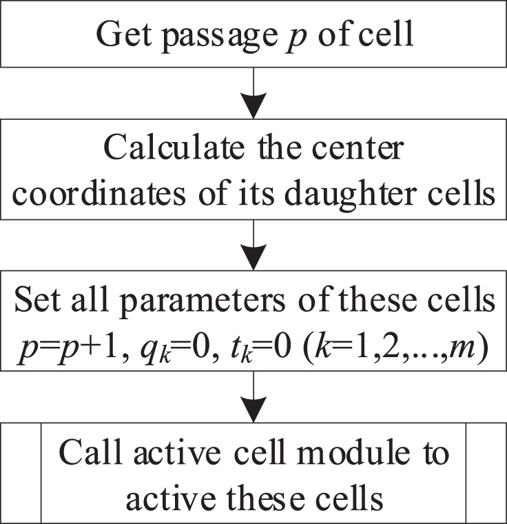
2.2.1 Training process

The main function of this process is to culture memory cells. Cells divide and renew under the active by antibodies, and some of them evolved into memory cells. There are two main modules in the training process, include the activated cell module, and the cell division model. The framework of the training process for n-dimensional data (n≤3) is described as follows.

Step 1: Initialization, assign value to pm and mcit, and initialize cell set C . The zero passage cell is initialized as < 0.5, 0.5, 0.5, 0, 0, 0, 0, 0, ... , 0, 0 > or<0.5, 0.5, 0, 0, 0, 0, 0, ... , 0, 0 > .

Step 2: To culture cells.

This step includes an activated cell module and a cell division model, and it is a recursive call. In this recursion pattern, two modules each call the other.

The main function of the activated cell module is that whether a cell that is activated by antibodies needs to divide according to cell division strategy. The flowchart of the activate cell module is shown in Fig. 2.

Fig. 2

The flowchart of the activated cell module.

The main function of the cell division module is to divide a cell into daughter cells, and initialization the parameters of its daughter cells. The flowchart of the cell division module is shown in Fig. 3.

Fig. 3

The flowchart of the cell division module.

During the training process, the recursive function calls are used a number of times. This training progress is described in [0, 1]² as shown in Fig. 4. There are 3 types of samples, and the training samples and the initial cell are shown in Fig. 4a. The parameter pm = 4, and the cell division progress is shown in Fig. 4b, 4c, and 4d. All cells are shown in Fig. 4e. Different colors represent different types of memory cells, and the white represents hollow cells. Squares of different sizes are different passage cells, the larger size of the square, and the higher passage of cell.

Fig. 4

The training process in [0, 1]².

There are 112 cells, and 58 of them are memory cells. The last activation time of all cells set as 0. Cell 1, cell 4 and cell 8 are hollow cells, they are recorded as < 0.125, 0.125, 2, 0, 0, 0, 0, 0, 0>,<0.3125, 0.0625, 3, 0, 0, 0, 0, 0, 0>,<0.40625, 0.09375, 4, 0, 0, 0, 0, 0, 0>, respectively. Cell 9, cell 49 and cell 99 are sole label memory cells, they are recorded as < 0.46875, 0.09375, 4, 0, 0, 0, 0, 1, 0>,<0.53125, 0.46875, 4, 0, 0, 2, 0, 0, 0>,<0.71875, 0.84375, 4, 4, 0, 0, 0, 0, 0>, respectively. Cell 76 is a multi-label memory cell, and has two types of information. It is recorded as < 0.71875, 0.71875, 4, 2, 0, 3, 0, 0, 0 > .

An n-dimensional cell will divide into 2 ⁿ daughter cells. This can lead to very low efficiency for high-dimensional data. In this paper, an n-dimensional (n > 3) data (d₁, d₂, …, d_n) will be divided into n fragments, (d₁, d₂, d₃), (d₂, d₃, d₄), ... , (d_n-2, d_n-1, d_n), (d_n-1, d_n, d₁), (d_n, d₁, d₂), and then these fragments are used to culture memory cells respectively. For example, a 20-dimensional cell will divide into 2²⁰ = 1048576 daughter cells, but only 20×2³ = 160 daughter cells are generated in this method. The flowchart of the training process for n-dimensional data (n > 3) is shown in Fig. 5.

Fig. 5

The flowchart of the training process for n-dimensional data (n > 3).

2.2.2 Testing process

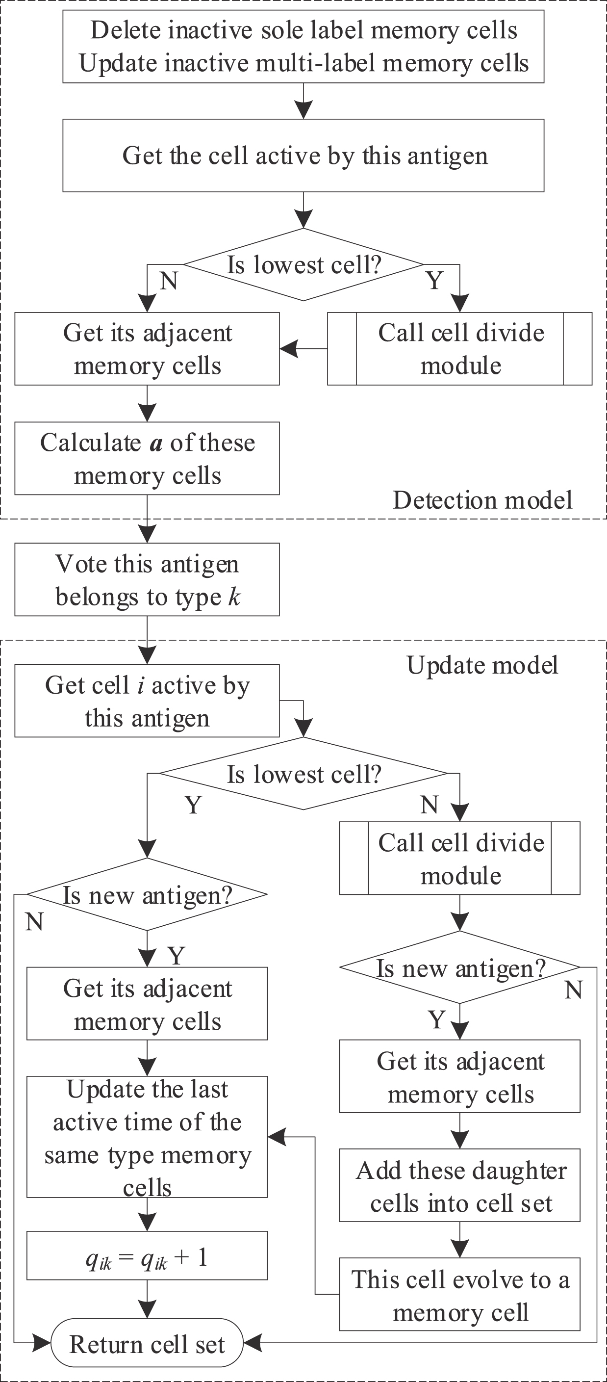
Memory cells can recognize and eliminate invaders very fast and more efficient when they attack the immune system again. The type of antigen can be recognized by the affinity between this antigen and memory cells. Memory cells are used to recognize antigens in the testing progress of CLCMTVD. The hollow cells which are attacked by antigens can evolve into memory cells, and some memory cells these are not active for some time can be updated, even eliminated during the testing stage.

The framework of the testing process for n-dimensional data (n≤3) is described as follows.

Step 1: To delete the inactive sole label memory cells, and update the inactive multi-label memory cells.

If the last activation time of sole label memory cells is more than mcit, these memory cells need to delete. The parameters of these cells set as 0, such as q_ik = 0, t_ik = 0. If the last activation time of one type of multi-label memory cells is more than mcit, these memory cells need to update. The parameters of this type of these memory cells set as 0, such as q_ij = 0, t_ij = 0.

Step 2: To obtain the cell this is attacked by antigen.

If antigen attacks a high passage hollow cell, this cell needs to divide according to the cell division strategy.

Step 3: To find adjacent memory cells of this cell, and return the affinity.

If this cell is a hollow cell, return the affinities of its adjacent memory cells. If this cell is a memory cell, return the affinities of its adjacent memory cells and this memory cell.

Step 4: To determine the type of this antigen.

The type of this antigen is voting by the affinities, it is the same as the memory cell with the highest affinity.

Step 5: To update the memory cells.

If the sampling time of this antigen is later than the last activation time of these memory cells, update the last activation time of this cell and its adjacent memory cells. If this cell is a hollow cell, it will evolve into a memory cell.

Step 1, Step 2 and Step 3 can be named as the detection model, and Step 5 can be named as the updated model. The flowchart of the testing process for n-dimensional data (n≤3) is shown in Fig. 6.

Fig. 6

The flowchart of the testing process for n-dimensional data (n≤3).

The testing progress is described in [0, 1]² as shown in Fig. 7. There are 3 types of samples, and the cells are cultured as shown in Fig. 7a. Suppose at t = 5, the brief descriptions of these memory cells are shown in the second column of Table 1. There are two antigens t₁ and t₂, and their sampling times are 6 and 7, respectively.

Fig. 7

The continual learning testing progress (pm = 3, mcit = 2).

Table 1

Descriptions of memory cells

Memory cells	t = 5	t = 6	t = 7
5	<0.5625, 0.0625, 3, 0, 0, 0, 0, 1, 5>	<0.5625, 0.0625, 3, 0, 0, 0, 0, 1, 5>	<0.5625, 0.0625, 3, 0, 0, 0, 0, 1, 7>
13	<0.4375, 0.5625, 3, 0, 0, 1, 4, 0, 0>	<0.4375, 0.5625, 3, 0, 0, 1, 4, 0, 0>
17	<0.5625, 0.5625, 3, 0, 0, 3, 5, 0, 0>	<0.5625, 0.5625, 3, 0, 0, 3, 6, 0, 0>	<0.5625, 0.5625, 3, 0, 0, 3, 6, 0, 0>
20	<0.6875, 0.6875, 3, 2, 4, 3, 5, 0, 0>	<0.6875, 0.6875, 3, 2, 4, 3, 6, 0, 0>	<0.6875, 0.6875, 3, 0, 0, 3, 6, 0, 0>
24	<0.9375, 0.6875, 3, 2, 5, 0, 0, 0, 0>	<0.9375, 0.6875, 3, 2, 5, 0, 0, 0, 0>	<0.9375, 0.6875, 3, 2, 6, 0, 0, 0, 0>
25	<0.8125, 0.8125, 3, 3, 4, 0, 0, 0, 0>	<0.8125, 0.8125, 3, 3, 4, 0, 0, 0, 0>
4	<0.8125, 0.4375, 3, 0, 0, 1, 6, 0, 0>	<0.9375, 0.8125, 3, 1, 6, 0, 0, 0, 0>
7	∼	∼	<0.5625, 0.1875, 3, 0, 0, 0, 0, 1, 7>

At t = 6, an antigen t₁ attacks cell 4, and this is a high passage hollow cell. Cell 4 divides into 4 daughter cells, cell 4, cell 29, cell 30 and cell 31. The adjacent memory cells of cell 4 include cell 17, cell 20 and cell 24, as shown in Fig. 7b. Antigen t₁ belongs to type 2, and cell 4 evolved into a memory cell, as shown in Fig. 7c. The last activation time of cell 4, cell 17 and cell 20 update to t = 6; the last activation time of cell 24 does not update for its type is not the same to cell 4, as shown in the third columns of Table 1.

At t = 7, an antigen t₂ attacks cell 7. The adjacent memory cell of cell 7 is cell 5, as shown in Fig. 7b. Antigen t₂ belongs to type 3, and cell 7 evolved into a memory cell, as shown in Fig. 7d. The last activation time of cell 5 and cell 7 update to t = 7. At the same time, cell 13, cell 20 and cell 25 inactive more than mcit. Cell 13 and cell 25 was eliminated, and Cell 20 was updated, as shown in the fourth columns of Table 1.

For n-dimensional data (n > 3), the last activation time of memory cells should be updated after determining the type of this antigen. The flowchart of the continual learning testing process for n-dimensional data (n > 3) is shown in Fig. 8.

Fig. 8

The flowchart of the testing process for n-dimensional data (n > 3).

When all data have the same sampling time (namely, data independent of time), CLCMTVD degenerates into a common supervised learning classification method. The memory cells cannot update during the testing stage.

3 Experiments

In order to determine the performance and possible advantages of the proposed method, we carried out the experiments on well-known datasets from UCI repository, synthetic data [8], and XJTU-SY rolling element bearing accelerated life test datasets [5] and compared our results to those obtained by other classical classification algorithms.

3.1 The basic classification performance

CLCMTVD is a continual learning classification method that is used for time-varying data space. When all data have the same sampling time (namely, data independent of time), CLCMTVD degenerates into a common supervised learning classification method. Therefore, it must have better classification performance like other supervised learning classification methods.

This section applies twenty standard data benchmark datasets to validate the proposed method. The results were compared to the classification methods including Naïve Bayesian networks (NB), C4.5 algorithm, kNN, RIPPER, back propagation algorithm (BP) and sequential minimal optimization algorithm (SMO).

3.1.1 The datasets

We tested the CLCMTVD on 20 well-known datasets without missing values from the UCI repository to assess its classification performance and possible advantages [8]. The brief descriptions of these datasets are shown in Table 2.

Table 2
Descriptions of datasets

Datasets Instances Features Classes

Balance 625 4 3

Diabetes 768 8 2

Haberman 306 3 2

Heart-statlog 270 13 2

Ionosphere 351 34 2

Iris 150 4 3

KR-vs-KP 3196 35 2

Letter 20000 16 26

Lymphotherapy 148 18 4

Monk1 124 6 2

Monk2 169 6 2

Monk3 122 6 2

Nursery 12960 8 5

Segment 2310 19 7

Sonar 208 60 2

Spambase 4601 57 2

Vehicle 846 18 4

Vowel 990 13 11

Waveform 5000 40 3

Wine 178 13 3

Datasets	Instances	Features	Classes
Balance	625	4	3
Diabetes	768	8	2
Haberman	306	3	2
Heart-statlog	270	13	2
Ionosphere	351	34	2
Iris	150	4	3
KR-vs-KP	3196	35	2
Letter	20000	16	26
Lymphotherapy	148	18	4
Monk1	124	6	2
Monk2	169	6	2
Monk3	122	6	2
Nursery	12960	8	5
Segment	2310	19	7
Sonar	208	60	2
Spambase	4601	57	2
Vehicle	846	18	4
Vowel	990	13	11
Waveform	5000	40	3
Wine	178	13	3

3.1.2 Data preprocessing

Every dataset was divided into ten mutually exclusive and equal-sized subsets. For each classification method, nine subsets were used to train, and one subset was used to test. Cross-validation was run 10 times for each method, the data averaged.

CLCMTVD has bad classification performances of KR-vs-KP and Spambase datasets when they are used to train directly. Most of the value in these two datasets is the same, this causes the fragments are similar. In this paper, these two datasets are preprocessing with Principal Component Analysis (PCA), and their principal component scores instead of these two datasets.

3.1.3 Effect of parameter pm on the classification performance

The basic classification performance of CLCMTVD is only related to parameter p m. It determines the quantity and quality of cells. The quantity of cells affects the run efficiency of CLCMTVD, and the quality of cells affects the precision rate of CLCMTVD.

The precision rate (P) is defined as follows: $P = \frac{TP}{TP + FP}$ (2)

Where TP is the number of true positives, FP is the number of false positives.

The main space consumption is used to store cells, and the data store space is related to pm, n, and m. For a n-dimension and m types datasets, the maximum store space is (n + m+1)*n*(2^pm) ³ (n > 3), and (2 + m+1)*(2^pm) ⁿ (n≤3).

Experiments were carried out on Balance, Ionosphere, Iris, Letter, Segment, and Wine datasets to illustrate the effects of parameter pm on the classification performance of CLCMTVD, as shown in Fig. 9. There is no obvious regular between precision rate and pm. At the moment, the value of pm depends on experience.

Fig. 9

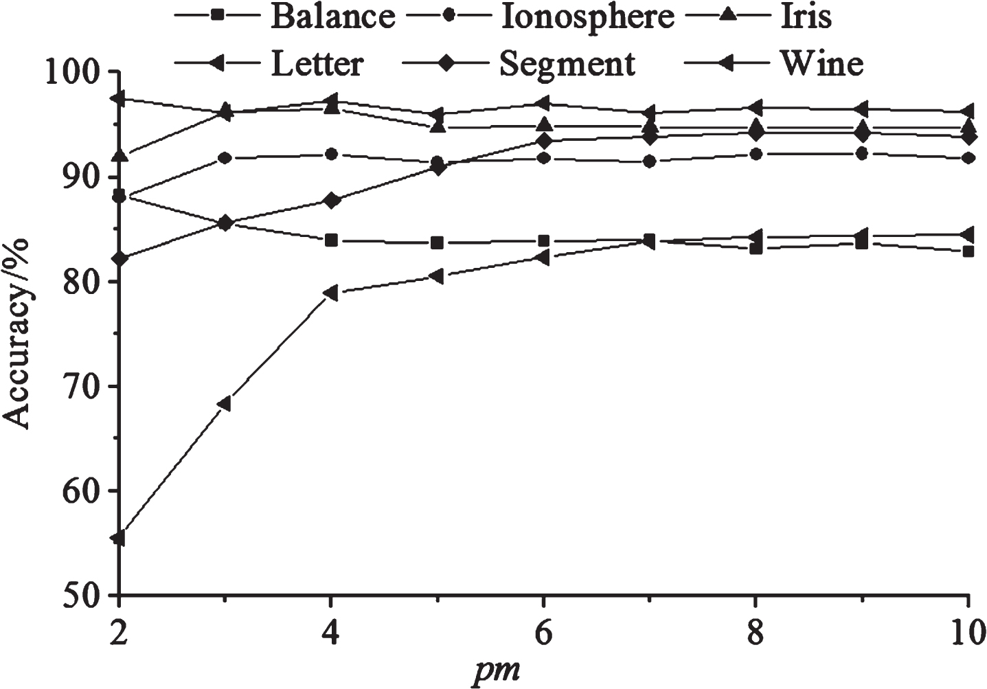
The effects of parameter p m on the classification performance of CLCMTVD.

3.1.4 The results

The results are shown in Table 3, and the results of other methods are from previous literature [31].

Table 3
The precision rate of each algorithm in each dataset (%)

Datasets NB C4.5 3NN RIPPER BP SMO CLCMTVD

Balance 90.53(±1.67) 77.82(±3.42) 86.74(±2.72) 80.91(±3.31) 85.67(±2.55) 87.62(±2.64) 88.27(pm = 2,±0.13)

Diabetes 75.75(±5.32) 74.49(±5.27) 73.86(±4.55) 75.22(±4.86) 77.04(±4.85) 77.07(±4.14) 74.49(pm = 6,±0.65)

Haberman 75.06(±5.42) 71.05(±5.20) 69.77(±5.72) 72.72(±5.90) 74.20(±6.27) 73.40(±1.06) 72.94(pm = 2,±0.21)

Heart-statlog 83.59(±5.98) 78.15(±7.42) 79.11(±6.77) 78.70(±6.62) 83.30(±6.20) 83.81(±5.59) 83.74(pm = 4,±0.37)

Ionosphere 82.17(±6.14) 89.74(±4.38) 86.02(±4.31) 89.30(±4.63) 87.07(±5.52) 87.93(±4.69) 92.19(pm = 9,±0.38)

Iris 95.53(±5.02) 94.73(±5.30) 95.20(±5.11) 93.93(±6.57) 84.80(±7.10) 84.87(±7.63) 96.53(pm = 4,±0.76)

KR-vs-KP 87.79(±1.91) 99.44(±0.37) 96.56(±1.00) 99.13(±0.44) 98.92(±0.60) 95.78(±1.20) 91.84(pm = 5,±0.21)

Letter 64.12(±0.94) 87.95(±0.61) 94.54(±0.23) 87.10(±0.45) 81.93(±0.62) 81.57(±0.19) 84.53(pm = 10,±0.09)

Lymphotherapy 83.13(±8.89) 75.84(±11.05) 81.74(±8.45) 77.36(±11.11) 82.26(±8.05) 85.94(±8.75) 80.41(pm = 10,±0.78)

Monk1 73.38(±12.49) 80.61(±11.34) 78.97(±11.89) 83.87(±16.34) 97.69(±5.99) 79.58(±11.99) 85.89(pm = 9,±2.22)

Monk2 56.83(±8.71) 57.75(±11.18) 54.74(±9.20) 56.21(±8.89) 100(±0.00) 58.70(±5.80) 63.96(pm = 4,±1.96)

Monk3 93.45(±6.57) 92.95(±6.68) 86.72(±9.99) 84.80(±9.27) 88.32(±8.49) 93.45(±6.57) 89.18(pm = 7,±1.15)

Nursery 90.30(±0.72) 97.18(±0.46) 97.36(±0.24) 98.67(±0.35) 99.43(±1.05) 93.02(±0.34) 92.75(pm = 5,±0.04)

Segment 80.16(±2.10) 96.79(±1.29) 96.12(±1.19) 95.53(±1.16) 91.35(±1.90) 89.72(±1.72) 94.29(pm = 8,±0.14)

Sonar 67.71(±8.66) 73.61(±9.34) 83.76(±8.51) 75.45(±10.01) 78.67(±9.21) 77.88(±8.45) 76.18(pm = 4,±1.28)

Spambase 79.56(±1.56) 92.68(±1.08) 89.80(±1.35) 92.67(±1.21) 91.22(±2.52) 90.48(±1.22) 90.97(pm = 10,±0.18)

Vehicle 44.68(±4.59) 72.28(±4.32) 70.21(±3.93) 68.32(±4.59) 81.11(±3.84) 74.08(±3.82) 71.23(pm = 6,±0.79)

Vowel 62.90(±4.38) 80.20(±4.36) 96.99(±2.13) 71.17(±5.14) 92.73(±3.14) 70.61(±3.86) 91.63(pm = 5,±0.45)

Waveform 80.01(±1.45) 75.25(±1.90) 77.67(±1.79) 79.14(±1.72) 86.56(±1.56) 86.94(±1.48) 81.63(pm = 4,±0.19)

Wine 97.46(±3.70) 93.20(±5.90) 95.85(±4.19) 93.14(±6.94) 98.02(±3.26) 98.76(±2.73) 97.57(pm = 2,±0.65)

Datasets	NB	C4.5	3NN	RIPPER	BP	SMO	CLCMTVD
Balance	90.53(±1.67)	77.82(±3.42)	86.74(±2.72)	80.91(±3.31)	85.67(±2.55)	87.62(±2.64)	88.27(pm = 2,±0.13)
Diabetes	75.75(±5.32)	74.49(±5.27)	73.86(±4.55)	75.22(±4.86)	77.04(±4.85)	77.07(±4.14)	74.49(pm = 6,±0.65)
Haberman	75.06(±5.42)	71.05(±5.20)	69.77(±5.72)	72.72(±5.90)	74.20(±6.27)	73.40(±1.06)	72.94(pm = 2,±0.21)
Heart-statlog	83.59(±5.98)	78.15(±7.42)	79.11(±6.77)	78.70(±6.62)	83.30(±6.20)	83.81(±5.59)	83.74(pm = 4,±0.37)
Ionosphere	82.17(±6.14)	89.74(±4.38)	86.02(±4.31)	89.30(±4.63)	87.07(±5.52)	87.93(±4.69)	92.19(pm = 9,±0.38)
Iris	95.53(±5.02)	94.73(±5.30)	95.20(±5.11)	93.93(±6.57)	84.80(±7.10)	84.87(±7.63)	96.53(pm = 4,±0.76)
KR-vs-KP	87.79(±1.91)	99.44(±0.37)	96.56(±1.00)	99.13(±0.44)	98.92(±0.60)	95.78(±1.20)	91.84(pm = 5,±0.21)
Letter	64.12(±0.94)	87.95(±0.61)	94.54(±0.23)	87.10(±0.45)	81.93(±0.62)	81.57(±0.19)	84.53(pm = 10,±0.09)
Lymphotherapy	83.13(±8.89)	75.84(±11.05)	81.74(±8.45)	77.36(±11.11)	82.26(±8.05)	85.94(±8.75)	80.41(pm = 10,±0.78)
Monk1	73.38(±12.49)	80.61(±11.34)	78.97(±11.89)	83.87(±16.34)	97.69(±5.99)	79.58(±11.99)	85.89(pm = 9,±2.22)
Monk2	56.83(±8.71)	57.75(±11.18)	54.74(±9.20)	56.21(±8.89)	100(±0.00)	58.70(±5.80)	63.96(pm = 4,±1.96)
Monk3	93.45(±6.57)	92.95(±6.68)	86.72(±9.99)	84.80(±9.27)	88.32(±8.49)	93.45(±6.57)	89.18(pm = 7,±1.15)
Nursery	90.30(±0.72)	97.18(±0.46)	97.36(±0.24)	98.67(±0.35)	99.43(±1.05)	93.02(±0.34)	92.75(pm = 5,±0.04)
Segment	80.16(±2.10)	96.79(±1.29)	96.12(±1.19)	95.53(±1.16)	91.35(±1.90)	89.72(±1.72)	94.29(pm = 8,±0.14)
Sonar	67.71(±8.66)	73.61(±9.34)	83.76(±8.51)	75.45(±10.01)	78.67(±9.21)	77.88(±8.45)	76.18(pm = 4,±1.28)
Spambase	79.56(±1.56)	92.68(±1.08)	89.80(±1.35)	92.67(±1.21)	91.22(±2.52)	90.48(±1.22)	90.97(pm = 10,±0.18)
Vehicle	44.68(±4.59)	72.28(±4.32)	70.21(±3.93)	68.32(±4.59)	81.11(±3.84)	74.08(±3.82)	71.23(pm = 6,±0.79)
Vowel	62.90(±4.38)	80.20(±4.36)	96.99(±2.13)	71.17(±5.14)	92.73(±3.14)	70.61(±3.86)	91.63(pm = 5,±0.45)
Waveform	80.01(±1.45)	75.25(±1.90)	77.67(±1.79)	79.14(±1.72)	86.56(±1.56)	86.94(±1.48)	81.63(pm = 4,±0.19)
Wine	97.46(±3.70)	93.20(±5.90)	95.85(±4.19)	93.14(±6.94)	98.02(±3.26)	98.76(±2.73)	97.57(pm = 2,±0.65)

Table 3 shows that the solutions obtained by the CLCMNLD are higher than the worst solutions that were obtained by the other algorithms. For Ionosphere and Iris datasets, CLCMTVD has the highest precision rate.

3.2 Experiments for time-varying synthetic data space

We tested the CLCMTVD on 2-dimensional time-varying synthetic data space to assess its classification performance and possible advantages. There are 3 types of samples, and the sample spaces at different dimensionless time are shown in Fig. 10.

Fig. 10

The sample spaces at different dimensionless time.

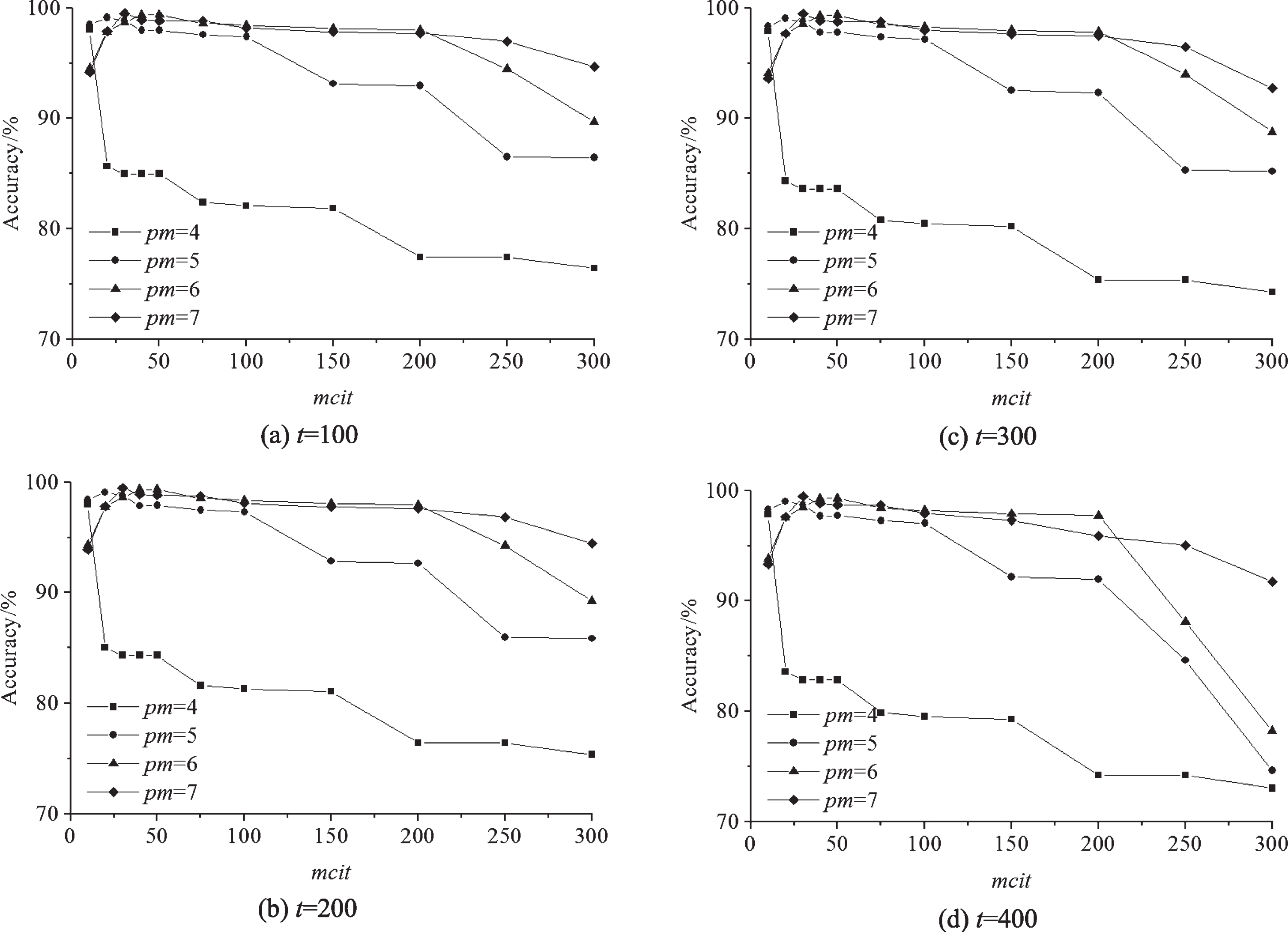
3.2.1 Effect of parameter pm and mcit on classification performance of CLCMTVD

CLCMTVD has two parameters, pm and mcit, need to be initialized. Parameter pm determines the size of memory cells, and mcit determines the speed of memory cells updating. Obviously, the number of cells and memory cells increases and the computational efficiency decrease with the increase of pm.

Eighty percent of samples from the first 100, 200, 300 and 400 dimensionless times randomly selected are used as training samples, and the rest samples are used as testing samples. All results were repeated 50 times, the data averaged. With the training samples from the first 100 dimensionless time as an example, the memory cells at different dimensionless time are shown in Fig. 11.

Fig. 11

The memory cells at different dimensionless time (pm = 4, mcit = 10).

The classification performances have similar change rules with different training samples when all the other settings are the same, as shown in Fig. 12. The classification performance of CLCMTVD is based on the relative position and quantity of the different types of memory cells. The number of memory cells increases with the mcit increase and reduce the classification performance.

Fig. 12

The classification performance with different parameters.

When pm = 4 the precision rate decreases with the mcit increase. This is because when pm is relatively small, the size of memory cells is relatively large. These memory cells occupy relative large spaces at some time. These spaces increase with the mcit increase and leading to low precision rate.

When pm = 5, pm = 6, and pm = 7 the precision rate increased firstly and decreased later with the mcit increase. This is because when pm is relatively large, the size of memory cells is relatively small. These memory cells occupy relative small spaces when mcit is relatively small, and they occupy relative large spaces when mcit is relatively large. All of these can lead to low precision rate.

When the memory cells and samples space change synchronous, CLCMTVD can get the best classification performance.

The classification performances change little with different training samples when all the other settings are the same because the memory cells evolve into a similar situation with the passage of time. Figures 13 –15 and 16 show the memory cells with different training samples at different dimensionless times, and parameter pm = 5 and mcit = 20.

Fig. 13

The memory cells at different time (Initial t = 100).

Fig. 14

The memory cells at different time (Initial t = 200).

Fig. 15

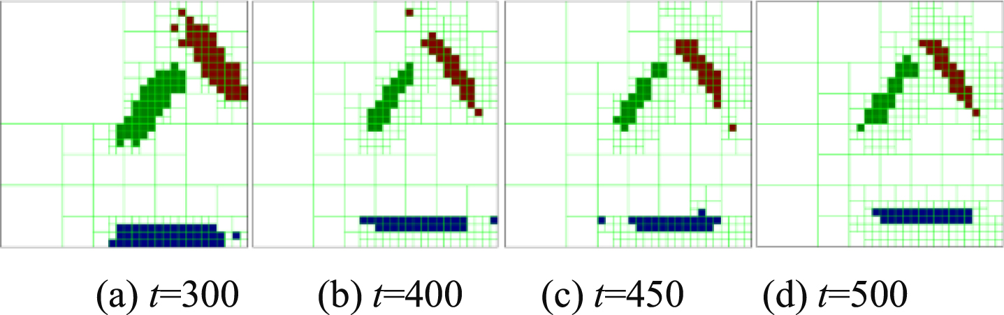
The memory cells at different time (Initial t = 300).

Fig. 16

The memory cells at different time (Initial t = 400).

Figures 13a, 14a, 15a and 16a shows the initial memory cells, and these memory cells are different. Figures 13d, 14d, 15d and 16d shows the memory cells at dimensionless time t = 500, and these memory cells become very similar after a period of time for evolution. Figures 13c, 14c and 15b also shows this phenomenon.

3.2.2 Classification performance of CLCMTVD

We tested the CLCMTVD on 2-dimensional time-varying synthetic data space as shown in Fig. 10. The samples from the first 100, 200, 300 and 400 dimensionless times are used as training samples, and the rest samples are used as testing samples. The results were compared to BP, SVM, CNN and LSTM.

BP has 9 neurons of the hidden layer. SVM has RBF kernel and the parameters c and g are determined by adopting the cross validation method. The samples are transformed to grayscale images with 28*28 pixels, and then 15 Layers CNN which includes 3 convolutional layers, 3 normalization layers, 3 active layers, 2 pooling layers and 1 fully connected layer was used to classify these images. Bidirectional LSTM has 100 hidden units and 20 batch size. The parameter pm and mcit of CLCMTVD are 5 and 20 respectively. We also take sampling time as an attribute of samples for BP and SVM, recorded as BPt and SVMt respectively. The results of BP, BPt, SVM, SVMt, CNN and LSTM were repeated 50 times, the data averaged. The results of CLCMTVD only calculated once, because the classification results and the memory cells generated by CLCMTVD are constant when the training samples and all parameters do not change.

Figure 17 and Table 4 show that CLCMTVD has the highest precision rate because CLCMTVD can continuously update its memory cells by learning testing data during the testing stage.

Fig. 17

The results of different methods.

Table 4

The results of different methods

Methods	The sampling time
	100	200	300	400
BP	54.34	52.12	50.76	50.37
BPt	49.31	55.29	58.67	60.86
SVM	55.39	42.47	34.57	31.51
SVMt	35.04	36.06	37.13	38.77
CNN	24.45	20.54	17.66	15.86
LSTM	54.43	54.39	55.04	54.54
CLCMTVD	99.11	99.06	99	98.96

3.3 Experiments for XJTU-SY rolling element bearing accelerated life test datasets

We tested the CLCMTVD on XJTU-SY rolling element bearing accelerated life test datasets to assess its classification performance and possible advantages.

3.3.1 The datasets

XJTU-SY rolling element bearing accelerated life test datasets [5] are provided by the Institute of Design Science and Basic Component at Xi’an Jiaotong University (XJTU), China and the Changxing Sumyoung Technology Co., Ltd. (SY) China.

The datasets were acquired by conducting many accelerated degradation experiments. A total of 3 different operating conditions were set in the accelerated degradation experiments, and 5 bearings were tested under each operating condition. We tested the CLCMTVD on one of them, and the brief descriptions of is shown in Table 5. Every instance includes horizontal vibration signals and vertical vibration signals.

Table 5
Descriptions of datasets

Datasets Instances Operating Condition

Bearing 3_1 2538 Radial force: 10kN

Bearing 3_2 2496 Rotating speed: 2400rmp

Bearing 3_3 371 Sampling frequency: 25.6kHz

Bearing 3_4 1515 Sampling period: 1 min

Bearing 3_5 114 ∼

Datasets	Instances	Operating Condition
Bearing 3_1	2538	Radial force: 10kN
Bearing 3_2	2496	Rotating speed: 2400rmp
Bearing 3_3	371	Sampling frequency: 25.6kHz
Bearing 3_4	1515	Sampling period: 1 min
Bearing 3_5	114	∼

3.3.2 Data preprocessing

The raw data is analyzed by “db16” wavelet for eight layers to get the high-frequency wavelet coefficients energy of each layer as the signal feature. The horizontal vibration signals and vertical vibration signals of each instance generate 8 signal features respectively. Every sample is composed of horizontal signal feature and vertical signal feature. All the samples are normalized to [0, 1]¹⁶.

3.3.3 The results and discussion

The first 40 samples from each datasets are used as training samples, and the rest samples are used as testing samples. The results were compared to BP, SVM, CNN and LSTM.

BP has 45 neurons of the hidden layer. SVM has RBF kernel and the parameters c and g are determined by adopting the cross validation method. The samples are transformed to grayscale images with 32*32 pixels, and then 15 Layers CNN which includes 3 convolutional layers, 3 normalization layers, 3 active layers, 2 pooling layers and 1 fully connected layer was used to classify these images. Bidirectional LSTM has 100 hidden units and 20 batch size. The parameter pm and mcit of CLCMTVD are 5 and 200 respectively.

Table 6 shows the detailed accuracy by class for every algorithm, including true positive rate (TPR), false positive rate (FPR), precision rate (P), recall rate (R), and F-Measure.

Table 6
The detailed accuracy by class for every algorithm

Algorithms Evaluation parameters Bearing 3_1 Bearing 3_2 Bearing 3_3 Bearing 3_4 Bearing 3_5

BP TPR 96.68 47.7 93.1 88.27 0.92

FPR 8.15 5.74 0.23 0.13 15.24

P 87.03 82.1 95.78 99.48 0.1

R 96.68 47.7 93.1 88.27 0.92

F-Measure 91.6 60.34 94.42 93.54 0.17

SVM TPR 94.67 43.38 95.63 79.93 0.92

FPR 5.39 4.6 12.6 0.17 9.82

P 90.86 83.87 29.49 99.25 0.15

R 94.67 43.38 95.63 79.93 0.92

F-Measure 92.73 57.18 45.08 88.55 0.25

CNN TPR 94.81 50.9 92.79 68.25 1.49

FPR 2.38 7.3 18.63 0.03 4.23

P 95.74 79.36 21.53 99.84 0.55

R 94.81 50.9 92.79 68.25 1.49

F-Measure 95.28 62.02 34.95 81.07 0.81

LSTM TPR 94.98 52.2 95.63 93.64 1.03

FPR 2.86 6.39 15.33 0.3 1.25

P 94.95 81.84 25.58 98.85 1.29

R 94.98 52.2 95.63 93.64 1.03

F-Measure 94.96 63.74 40.36 96.17 1.15

CLCMTVD TPR 100 100 92.11 100 0.92

FPR 0 3.03 0 0 0

P 100 94.79 100 100 100

R 100 100 92.11 100 0.92

F-Measure 100 97.33 95.89 100 1.82

Algorithms	Evaluation parameters	Bearing 3_1	Bearing 3_2	Bearing 3_3	Bearing 3_4	Bearing 3_5
BP	TPR	96.68	47.7	93.1	88.27	0.92
	FPR	8.15	5.74	0.23	0.13	15.24
	P	87.03	82.1	95.78	99.48	0.1
	R	96.68	47.7	93.1	88.27	0.92
	F-Measure	91.6	60.34	94.42	93.54	0.17
SVM	TPR	94.67	43.38	95.63	79.93	0.92
	FPR	5.39	4.6	12.6	0.17	9.82
	P	90.86	83.87	29.49	99.25	0.15
	R	94.67	43.38	95.63	79.93	0.92
	F-Measure	92.73	57.18	45.08	88.55	0.25
CNN	TPR	94.81	50.9	92.79	68.25	1.49
	FPR	2.38	7.3	18.63	0.03	4.23
	P	95.74	79.36	21.53	99.84	0.55
	R	94.81	50.9	92.79	68.25	1.49
	F-Measure	95.28	62.02	34.95	81.07	0.81
LSTM	TPR	94.98	52.2	95.63	93.64	1.03
	FPR	2.86	6.39	15.33	0.3	1.25
	P	94.95	81.84	25.58	98.85	1.29
	R	94.98	52.2	95.63	93.64	1.03
	F-Measure	94.96	63.74	40.36	96.17	1.15
CLCMTVD	TPR	100	100	92.11	100	0.92
	FPR	0	3.03	0	0	0
	P	100	94.79	100	100	100
	R	100	100	92.11	100	0.92
	F-Measure	100	97.33	95.89	100	1.82

The recall rate (R) and F-Measure are defined as follows: $TPR = \frac{TP}{TP + FN}$ (3) $FPR = \frac{FP}{FP + TN}$ (4) $R = \frac{TP}{TP + FN}$ (5) $F - measure = \frac{2 * P * R}{P + R}$ (6) where, FN is the number of false negatives.

Table 6 shows that CLCMTVD has the better classification performance.

4 Conclusions and future works

In this paper, we proposed a continual learning classification method for time-varying data space based on artificial immune system, named CLCMTVD. It can change a linearly inseparable spatial problem into many classification problems of several different times, and most of them are linearly separable spatial problems.

We carried out the experiments on well-known datasets from the UCI repository, synthetic data and XJTU-SY rolling element bearing accelerated life test datasets to assess the performance and possible advantages of CLCMTVD. The results of experiments on well-known datasets from the UCI repository show that CLCMTVD has better classification performance when it degenerates into a common supervised learning classification method. The result of experiments on 2-dimensional synthetic data and XJTU-SY rolling element bearing accelerated life test datasets show that CLCMTVD has the best classification performance for time-varying data space.

It is noteworthy that the CLCMTVD is incomplete. There are many future woks to do to improve it. The model only uses very simple classification strategies; it should combine with other classification methods to expand its advantage. It should be improved to apply to more complex time-varying data space.

Footnotes

Acknowledgments

This work was sponsored by the National Natural Science Foundation of China (Grant No. 52075310).

References

Darwiche

, Bayesian networks, Communications of the ACM 53(12) (2010), 80–90.

Jeyasothy

, Sundaram

and Sundararajan

, SEFRON: A new spiking neuron model with time-varying synaptic efficacy function for pattern classification, IEEE Transactions on Neural Networks and Learning Systems 30(4) (2018), 1231–1240.

Jain

A.K.

, Duin

R.P.W.

and Mao

J.C.

, Statistical pattern recognition: A review, IEEE Transactions on Pattern Analysis and Machine Intelligence 22(1) (2000), 4–37.

Liu

, Lifelong machine learning: a paradigm for continuous learning, Frontiers of Computer Science 11(3) (2017), 359–361.

Wang

, Lei

Y.G.

, Li

N.P.

and Li

N.B.

, A hybrid prognostics approach for estimating remaining useful life of rolling element bearings, IEEE Transaction on Reliability 69(1) (2020), 401–412.

Dasgupta

, Advances in artificial immune systems, IEEE Computational Intelligence Magazine 1(4) (2006), 40–49.

Dasgupta

, Yu

S.H.

and Nino

, Recent advances in artificial immune systems: models and applications, Applied Soft Computing 11(2) (2011), 1574–1587.

Dua

and Graff

, UCI Machine Learning Repository. http://archive.ics.uci.edu/ml.

, Liu

S.L.

and Zhang

H.L.

, A method of anomaly detection and fault diagnosis with online adaptive learning under small training samples, Pattern Recognition 64 (2017), 374–385.

10.

Mishra

D.P.

and Ray

, P, Fault detection, location and classification of a transmission line, Neural Computing & Applications 30(5) (2018), 1377–1424.

11.

Parisi

G.I.

, Kemker

, Part

J.L.

, Kanan

and Wermter

, Continual lifelong learning with neural networks: A review, Neural Networks 113 (2019), 54–71.

12.

Qian

, Lu

S.L.

, Pan

D.H.

, Tang

S.S.

, Liu

Y.B.

and Wang

Q.J.

, Edge computing: a promising framework for real-time fault diagnosis and dynamic control of rotating machines using multi-sensor data, IEEE Sensors Journal 19(11) (2019), 4211–4220.

13.

Izonin

, Trostianchyn

, Duriagina

, Tkachenko

, Tepla

and Lotoshynska

, The combined use of the wiener polynomial and SVM for material classification task in medical implants production, International Journal of Intelligent Systems and Applications 10(9) (2018), 40–47.

14.

Sun

J.C.

, Yang

, Liu

Y.Q.

, Chen

C.L.

, Rao

W.Y.

and Bai

Y.H.

, Univariate time series classification using information geometry, Pattern Recognition 95 (2019), 24–35.

15.

Nalepa

and Kawulok

, Selecting training sets for support vector machines: a review, Artificial Intelligence Review 52(2) (2019), 857–900.

16.

Zheng

J.Q.

, Chen

Y.F.

and Zhang

, A survey of artificial immune applications, Artificial Intelligence Review 34(1) (2010), 19–34.

17.

Schmidhuber

, Deep learning in neural networks: An overview, Neural networks 61 (2015), 85–117.

18.

Zhou

and Dasgupta

, Revisiting negative selection algorithms, Evolutionary Computation 15(2) (2007), 223–251.

19.

Yan

, Ji

Z.W.

, Lu

H.J.

, Huang

, Shen

and Xue

, Fast and accurate classification of time series data using extended elm application in fault diagnosis of air handling units, IEEE Transactions on systems man cybernetics-systems 49(7) (2019), 1349–1356.

20.

Feng

L.J.

, Zhao

C.H.

, Chen

C.L.P.

, Li

Y.L.

, Zhou

, Qiao

H.L.

and Fu

, BNGBS: an efficient network boosting system with triple incremental learning capabilities for more nodes, samples, and classes, Neurocomputing 412 (2020), 486–501.

21.

Elshenawy

L.M.

and Mahmoud

T.A.

, Fault diagnosis of time-varying processes using modified reconstruction-based contributions, Journal of Process Control 70 (2018), 12–23.

22.

Rutkowski

, Adaptive probabilistic neural networks for pattern classification in time-varying environment, Neural Networks 15(4) (2004), 811–827.

23.

Amer

and Maul

, A review of modularization techniques in artificial neural networks, Artificial Intelligence Review 52(1) (2019), 527–561.

24.

Jordan

M.I.

and Mitchell

T.M.

, Machine learning: Trends, perspectives, and prospects, Science 349(6245) (2015), 255–260.

25.

Bayar

, Darmoul

, Hajri-Gabouj

and Pierreval

, Fault detection, diagnosis and recovery using artificial immune systems: A review, Engineering Applications of Artificial Intelligence 46 (2015), 43–57.

26.

Hatami

, Gavet

and Debayle

, Bag of recurrence patterns representation for time-series classification, Pattern Analysis and Applications 22 (2019), 877–887.

27.

Duda

, Rutkowski

, Jaworski

and Rutkowska

, On the parzen kernel-based probability density function learning procedures over time-varying streaming data with applications to pattern classification, IEEE Transactions on Cybernetics 50(4) (2020), 1683–1696.

28.

Skryjomski

, Krawczyk

and Cano

, Speeding up-nearest neighbors classifier for large-scale multi-label learning on GPUs, Neurocomputing 354 (2019), 10–19.

29.

Zhang

Q.C.

, Zhou

J.L.

, Wang

and Chai

T.Y.

, Output feedback stabilization for a class of multi-variable bilinear stochastic systems with stochastic coupling attenuation, IEEE Transactions on Automatic Control 62(6) (2016), 2936–2942.

30.

Tkachenko

, Doroshenko

, Izonin

, Tsymbal

and Havrysh

, Imbalance data classification via neural-like structures of geometric transformations model: Local and global approaches, Proceeding of 1st International Conference on Computer Science, Engineering and Education Applications, Springer, 2018, 112–122.

31.

Kotsiantis

S.B.

, Zaharakis

I.D.

and Pintelas

P.E.

, Machine learning: a review of classification and combining techniques, Artificial Intelligence Review 26(3) (2016), 159–190.

32.

Xiao

S.G.

, Liu

S.L.

, Song

M.M.

, Nie

and Zhang

H.L.

, Coupling rub-impact dynamics of double translational joints with subsidence for time-varying load in a planar mechanical system, Multibody System Dynamics 48(4) (2020), 451–486.

33.

S.H.

and Wang

, A new support vector machine model and its application in time-varying signal classification, Proceeding of 2008 Fourth International Conference on Natural Computation, IEEE, 2008, 416–420.

34.

Kabir

and Papadopoulos

, Applications of Bayesian networks and Petri nets in safety, reliability and risk assessments: A review, Safety Scicence 115 (2019), 154–175.

35.

Shahid

S.M.

, Ko

and Kwon

, Real-time classification of diesel marine engine loads using machine learning, Sensors 19(14) (2019), 3172.

36.

W.K.

and Zhao

C.H.

, Broad convolutional neural network based industrial process fault diagnosis with incremental learning capability, IEEE Transactions on Industrial Electronics 67(6) (2020), 5081–5091.

37.

Yin

, Zhang

Q.C.

, Wang

and Ding

Z.T.

, Rbfnn-based minimum entropy filtering for a class of stochastic nonlinear systems, IEEE Transactions on Automatic Control 65(1) (2019), 376–381.

38.

Yuan

X.Y.

, Emotional tendency of online legal course review texts based on SVM algorithm and network data acquisition, Journal of Intelligent & Fuzzy Systems 37(5) (2019), 6253–6263.

39.

Wang

X.Y.

, Liang

X.X.

and Sun

J.Z.

, A new approach of neural networks to time-varying database classification, Proceeding of 2005 International Conference on Machine Learning and Cybernetics, IEEE, 2005, 2050–2054.

40.

Bengio

, Buhmann

J.M.

, Embrechts

and Zurada

J.M.

, Introduction to the special issue on neural networks for data mining and knowledge discovery, Neural Networks 11(3) (2000), 545–549.

41.

LeCun

, Bengio

and Hinton

, Deep learning, Nature 521(7553) (2015), 436–444.

42.

Liu

, Chen

S.Q.

, Guan

and Xu

, Layout optimization of large-scale oil-gas gathering system based on combined optimization strategy, Neurocomputing 332 (2019), 159–183.

43.

Zhou

Y.Y.

, Zhang

Q.C.

, Wang

, Zhou

and Chai

T.Y.

, Ekf-based enhanced performance controller design for nonlinear stochastic systems, IEEE Transactions on Automatic Control 63(4) (2017), 1155–1162.

44.

Chai

and Zhao

C.H.

, Multiclass oblique random forests with dual-incremental learning capacity, IEEE Transactions on Neural Networks and Learning Systems. DOI: 10.1109/TNNLS.2020.2964737.

Continual learning classification method for time-varying data space based on artificial immune system

Abstract

Keywords

1 Introduction

2.1 Definitions

2.2.1 Training process

3.1 The basic classification performance

3.1.1 The datasets

3.1.3 Effect of parameter pm on the classification performance

3.3.1 The datasets

Table 5 Descriptions of datasets Datasets Instances Operating Condition Bearing 3_1 2538 Radial force: 10kN Bearing 3_2 2496 Rotating speed: 2400rmp Bearing 3_3 371 Sampling frequency: 25.6kHz Bearing 3_4 1515 Sampling period: 1 min Bearing 3_5 114 ∼

3.3.3 The results and discussion

Footnotes

Acknowledgments

References

Table 5
Descriptions of datasets

Datasets Instances Operating Condition

Bearing 3_1 2538 Radial force: 10kN

Bearing 3_2 2496 Rotating speed: 2400rmp

Bearing 3_3 371 Sampling frequency: 25.6kHz

Bearing 3_4 1515 Sampling period: 1 min

Bearing 3_5 114 ∼