GMM with parameters initialization based on SVD for network threat detection

Abstract

In the field of security, the data labels are unknown or the labels are too expensive to label, so that clustering methods are used to detect the threat behavior contained in the big data. The most widely used probabilistic clustering model is Gaussian Mixture Models(GMM), which is flexible and powerful to apply prior knowledge for modelling the uncertainty of the data. Therefore, in this paper, we use GMM to build the threat behavior detection model. Commonly, Expectation Maximization (EM) and Variational Inference (VI) are used to estimate the optimal parameters of GMM. However, both EM and VI are quite sensitive to the initial values of the parameters. Therefore, we propose to use Singular Value Decomposition (SVD) to initialize the parameters. Firstly, SVD is used to factorize the data set matrix to get the singular value matrix and singular matrices. Then we calculate the number of the components of GMM by the first two singular values in the singular value matrix and the dimension of the data. Next, other parameters of GMM, such as the mixing coefficients, the mean and the covariance, are calculated based on the number of the components. After that, the initialization values of the parameters are input into EM and VI to estimate the optimal parameters of GMM. The experiment results indicate that our proposed method performs well on the parameters initialization of GMM clustering using EM and VI for estimating parameters.

Keywords

Network threat detection gaussian mixture models expectation maximization variational inference singular value decomposition parameters initialization

1 Introduction

With the rapid development of new generation information technology, such as mobile internet, big data, cloud computing and artificial intelligence, the service and applications of network and data are growing explosively. Meanwhile, malicious network activities and network policy violations have been frequently exposed, such as extortion virus attacks, data leakage, Botnet traffic attack, which have brought great challenges to the cybersecurity. Consequently, Intrusion Detection Systems (IDSs) have emerged with a group of methods to detect the intruders who break the computer system or misuse the system resources [1, 2]. One of the popular intrusion detection methods is to use machine learning and data mining techniques for Internet traffic malicious/benign classification based on the statistical traffic characteristics [2 –5].

Generally, machine learning and data mining techniques can be divided into classification and clustering [6]. Classification analysis is known as supervised learning methods, which deal with already labeled or classified data. The goal of the classification is to determine a certain object to belong to the explicit group. Clustering analysis is known as unsupervised learning methods, which do not depend on the predefined labels. And the objective is to calculate the difference between the data and to classify data into groups based on the similarity or dissimilarity measures [7 –9]. Once the data labels are not known, the clustering analysis methods can only be used.

The clustering methods can be divided into three general categories: partitional methods evaluating partitions based on some criterion, distance-based methods calculating the distance between clusters, and parametric model based methods built via probabilistic mixture models [7 , 10]. The most widely used probabilistic mixture model is Gaussian Mixture Models(GMM) [10 , 12–15], which is a probabilistic model assuming all the data samples fitting a mixture of a finite number of Gaussian distributions with unknown parameters. GMM is flexible and powerful to apply prior knowledge for modeling the uncertainty of the data. The advantage of GMM is that the amount of learning parameters is small and the involved parameters can be efficiently estimated [16]. Many researches on mixture models have given attention to the parameters estimation. Commonly, Expectation Maximization (EM) is considered an efficient algorithm to estimate the parameters of GMM by maximizing the log-likelihood function [17, 18]. Afterwards, Variational Inference (VI) has been proposed to estimate the value of the parameters through maximizing the evidence of lower bound in a coordinate ascend mechanism [19 –21]. However, both EM and VI are quite sensitive to initial values in the iterative updating of parameters, and the performance of GMM clustering method strongly depends on the initial starting points [10 , 23–25]. Therefore, we concentrate on the parameters initialization while EM and VI are used to estimate the optimal parameters of GMM.

In the process of GMM parameters estimation, a critical issue is to determine a proper number of GMM components. Generally, the larger the number is, the greater amount of calculation on all components is, and the higher the fitness of GMM is to the data in learning stage. Furthermore, the calculation load is higher and under-fitting may occur in the testing stage. Therefore, it is important to choose the proper value of GMM components number. In most cases, the value of the components number is set to a random value, which does not satisfy the data distribution neither lead to overfitting and poor generalization [26, 27]. In [28], Bayesian Information Criterion (BIC) is used to choose proper number from a series of comparisons on the GMM clustering results. However, this method often leads to get an unreasonably high number of poorly components. In [23], a robust EM clustering algorithm is developed to automatically obtain an optimal number of clusters. On the whole, all initialization techniques can be generally divided into deterministic and stochastic [13, 27]. The deterministic initialization methods estimate the start points based on the results from the clustering algorithms, such as hierarchical clustering [29]. The disadvantage of the deterministic methods is that they can not be compatible with other possible initial values, which may lead to an incorrect solution for the final results. The stochastic initialization methods choose the start points from any one in the parameter space. The choosing rule is to try different starting values and finally determine the one that yields the best results, such as BIC [28]. Because of the initialization steps repeating several times, the choosing procedures of BIC need to cost more time and computing resources comparing with the deterministic methods. In addition, there are some other initialization techniques in the literature referring to some more comprehensive reviews [13 , 31]. However, there are few papers to compare the proposed initialization techniques to asses which one is the best method. That is because some methods lack the compatibility, that are only suitable for some special scenarios. In this paper, we try to solve the compatibility problem based on Singular Value Decomposition (SVD) to make our initialization method suitable for a variety of data sets, such as high-dimensional. SVD is considered as a popular deterministic initialization method for Nonnegative Matrix Factorization (NMF) [32, 33]. SVD can factorize the data matrix into the form of multiplication of three matrices, including left-singular matrix, singular values matrix and right-singular matrix. These matrices can be interpreted as the features and clusters of the data sets. Therefor, we apply SVD to initialize the parameters of GMM.

GMM has several parameters to learn. In addition to considering the number of components, the initialization of the means and variances in GMM is also important. When the number of GMM components is determined, it means that the data can been divide into multiple initial clusters. The means and variances of the initial clusters from the data can be calculated. By definition, there is only one way to calculate the row mean by computing the average of the elements along the row axis and returning a row vector. Unlike the mean, the variance has many structures, such as diagonal, compound-symmetry, unstructured, time-series, and spatial [34]. For a whole data set composed of several clusters, the variance of the data set also has multiple types. For example, each cluster has its own general covariance matrix, all clusters share the same general covariance matrix, each cluster has its own diagonal covariance matrix and each cluster has its own single variance [35]. In this paper, we choose the type that each cluster has its own general covariance matrix. And we calculate the covariance matrix of each cluster through the classical maximum likelihood estimator, which is an unbiased estimator of the corresponding clusters’ covariance matrix [36].

Based on the above analysis, in this paper, we propose a new parameters initialization method based on SVD for GMM on the network threat detection. Firstly, GMM is built which contains several parameters, such as the number of GMM components, the mixing coefficients of the components, the mean of each component and the covariance of each component. Secondly, we use SVD to factorize the data matrix. Then we obtain the number of GMM components according to the singular values matrix. Meanwhile, the data are divided into several initial clusters. Next, we calculate the mean of each component according to the definition. And we calculate the covariance of each component through the classical maximum likelihood estimator, respectively. Thirdly, based on the initialization values of the parameters, EM and VI are used to continue to inference the optimal parameters of GMM, respectively, until GMM converges to its maximum output value and the optimal values of the parameters reaching steady state. Once these parameters are estimated, they are used to assign the network data samples into threat group or normal group based on the posterior probabilities of inclusion. The experiment results indicate that our proposed initialization method based on SVD provides more accurate parameter initialization, better generalization for GMM, lower computational complexity and less running time.

The rest of this paper is structured as follows. In Section 2 we introduce GMM for the data set containing several parameters, then EM and VI are used to inference the optimal values of the parameters. In section 3 we propose the parameters initialization method based on SVD. In section 4 we describe the overall solution framework of the model. In section 5 we describe the experiment setting and results in detail. In section 6 we conclude the paper.

2 GMM and parameters inference

In this section, we firstly introduce GMM for the data sets, containing several parameters. Then, we describe the process of EM algorithm to estimate the optimal values of the parameters. Next, we describe the process of VI algorithm to estimate the optimal values of the parameters.

2.1 GMM

GMM is powerful model-based to draw the entire data set to solve the clustering problem, while the clustering problem is reduced to estimate the parameters of the GMM. Suppose data set X = (x₁, x₂, …, x_n, … x_N), x_n = (x_n1, x_n2, …, x_nD) ^T, n = (1, 2, …, N) contains N independent D-dimensional samples, which are divided into Kclusters. The data is identically distributed by the multivariate Gaussian mixture model, which is a linear combination of more than one Gaussian distribution [37]. The Probability Density Function (PDF) is given by $f (X) = \sum_{k = 1}^{K} π_{k} N_{k} (x_{n}; μ_{k}, \sum_{k})$ (1) where $N_{k} (•)$ represents the PDF of the kth GMM component in the following form [38] $N_{k} (x_{n}; μ_{k}, \sum_{k}) = \frac{1}{(2 π)^{D / 2} | Σ_{k} |^{1 / 2}}$ $\cdot exp {- \frac{1}{2} (x - μ_{k})^{T} Σ_{k}^{- 1} (x - μ_{k})}$ (2)

In (1) and (2), K is the number of GMM components, π_k is the mixing coefficients of the kth component satisfying the constrains 0 ≤ π_k ≤ 1 and $\sum_{k = 1}^{K} π_{k} = 1$ , μ_k is the kth D-dimensional mean vector and ∑_k is the kth D × D covariance matrix. |Σ_k| is the determinant of the matrix ∑_k. Next, the goal is to estimate the parameters containing K, π_k, μ_k and ∑_k. Finally, the data set is classified into their correct clusters by the determined GMM.

2.2 EM for GMM

EM algorithm is considered to be the most effective method of parameter estimation, which operates with the complete-data log likelihood function, starting from parameters with initial values and iterating through E-step and M-step. The complete-data log likelihood function of N data samples is given by [34, 38] $L (x_{n}; μ_{k}, \sum_{k}) = \sum_{n = 1}^{N} log (\sum_{k = 1}^{K} π_{k} N_{k} (x_{n}; μ_{k}, \sum_{k}))$ (3)

At the E-step, EM calculates posterior probabilities that the nth sample belongs to the kth component. For GMM, the posterior probabilities are calculated by $π_{nk}^{(s)} = \frac{π_{k}^{(s)} N_{k} (x_{n}; μ_{k}^{(s - 1)}, \sum_{k}^{(s - 1)})}{\sum_{k^{'}}^{K} π_{k^{'}}^{(s - 1)} N_{k} (x_{n}; μ_{k^{'}}^{(s - 1)}, \sum_{k^{'}}^{(s - 1)})}$ (4) where n = 1, 2, . . . , N, k = 1, 2, . . . , K . s = 1, 2, . . . represents the iteration number. At the M-step, the conditional expected value of the complete-data log likelihood function given the data is maximized. For GMM, the formulas for updating mixing coefficients π_k, the mean vector μ_k and covariance matrix ∑_k are given as follows $π_{k}^{(s)} = \frac{\sum_{n = 1}^{N} π_{nk}^{(s)}}{N}$ (5) $μ_{k}^{(s)} = \frac{\sum_{n = 1}^{N} π_{nk}^{(s)} x_{n}}{\sum_{n = 1}^{N} π_{nk}^{(s)}}$ (6) $\sum_{k}^{(s)} = \frac{\sum_{n = 1}^{N} π_{nk}^{(s)} (x_{n} - μ_{k}^{(s)}) (x_{n} - μ_{k}^{(s)})^{'}}{\sum_{n = 1}^{N} π_{nk}^{(s)}}$ (7) where s denotes the iteration number. The loop is terminated when the convergence condition is satisfied. Then EM obtains the maximum likelihood estimates for all the parameters. And then the concrete GMM can be determined. According to the Bayes decision rule, every sample is assigned to the GMM component according to the highest posterior probability.

In (4)-(6), we note that the value of highest posterior probability depends on the parameters π_k, μ_k and ∑_k. In some situation,one drawback of EM is that it converges slowly, so that many algorithms have been proposed to speed up the convergence while keeping its simplicity [38]. Another drawback of EM is that the solution highly depends on the initial values of the parameters and consequently produce sub-optimal maximum likelihood estimates [10, 27]. To overcome these limitations, it needs to propose a new method to set the proper initial position for the parameters, which is also helpful to speed up the convergence. In this paper, we pay much attention to calculate the initial values of parameters K, π_k, μ_k and ∑_k.

2.3 VI for GMM

In the EM algorithm, it needs to calculate the expectation of the complete-data log likelihood with respect to the posterior of the latent variables. However, in some practice instance, the dimension of the data set is too high, or the posterior distribution has a highly complex form, so that it is hard to compute the expectation. In such situation, approximation schemes are considered effective to solve these problems. One of the widely applied approximation techniques is Variational Inference(VI), which uses more global criteria to computer the posterior [26, 39].

In this paper, we calculate the variational inference approximation solution for (1). Our goal is to infer the posterior distribution for the mean vector μ_k and the covariance matrix ∑_k, given the samples x_n drawn independently [38 , 41].

In VI framework, X = (x₁, x₂, …, x_N) is regarded as data set. For each sample x_n, it has a corresponding latent variable z_n, which comprises a l-of-K binary vector with elements Z = {z_nk}, k = 1, 2, . . . , K. z_n, π_k, μ_k and ∑_k are regarded as latent variables as well as parameters, and can be written as Θ = {Z, π_k, μ_k, ∑_k}. The mixture model can be denoted as p (X|Θ), the goal is to find an approximation for the posterior distribution p (X|Θ) as well as for the model evidence p (X). Then we introduce conjugate prior distributions over the parameters Z, π_k, μ_k, ∑. The analysis will be become considerably simplified.

Dirichlet distribution is used over the mixing coefficient π_k as follows [39] $p (π | α) = \frac{Γ (\sum_{k = 1}^{K} α_{k})}{\prod_{k = 1}^{K} Γ (α_{k})} \prod_{k = 1}^{K} π_{k}^{α_{k} - 1}$ (8) where α_k is the parameter for the kth component.

Similarly, an independent Gaussian-Wishart prior is used to control the mean μ_k and covariance ∑_k of each component as follows $\begin{matrix} p (μ_{k}, \sum_{k}) = p (μ_{k} | \sum_{k}) p (\sum_{k}) \\ = \prod_{k = 1}^{K} N (μ_{k} | m_{0}, β_{0}^{- 1} \sum_{k}) W (\sum_{k} | w_{0}, v_{0}) \end{matrix}$ (9) where m₀, β0, w0 and v₀ are the parameters of GMM.

According to the general expression for the optimal solution $q_{j}^{*} (Θ_{j})$ , Θ = {Z, π_k, μ_k, ∑_k}as follows $ln q_{j}^{*} (Θ_{j}) = E_{i \neq j} [ln p (X, Θ)] + const$ (10) $q_{j}^{*} (Θ_{j}) = \frac{exp (E_{i \neq j} [ln p (X, Θ)])}{\int exp (E_{i \neq j} [ln p (X, Θ)]) d Θ_{j}}$ (11) where $E_{i \neq j} [•]$ is the expectation with

respect to all the distributions of $q_{j}^{*} (Θ_{j})$ except for i ≠ j [42].

We obtain the variational update equations of the intermediate parameters, given by

$\begin{matrix} ln ρ_{nk} = E [ln π_{k}] + \frac{1}{2} E [ln | \sum_{k}^{- 1} |] - \frac{D}{2} ln (2 π) \\ - \frac{1}{2} E μ_{k}, \sum_{k} [(x_{n} - μ_{k})^{T} \sum_{k}^{- 1} (x_{n} - μ_{k})] \end{matrix}$ (12) $r_{nk} = \frac{ρ_{nk}}{\sum_{j = 1}^{K} ρ_{nj}}$ (13) $N_{k} = \sum_{n = 1}^{N} r_{nk}$ (14) ${\bar{x}}_{k} = \frac{1}{N_{k}} \sum_{n = 1}^{N} r_{nk} x_{n}$ (15) $S_{k} = \frac{1}{N_{k}} \sum_{n = 1}^{N} r_{nk} (x_{n} - {\bar{x}}_{k}) (x_{n} - {\bar{x}}_{k})^{T}$ (16) $α_{k} = α_{0} + N_{k}$ (17) $β_{k} = β_{0} + N_{k}$ (18) $m_{k} = \frac{1}{β_{k}} (β_{0} m_{0} + N_{k} {\bar{x}}_{k})$ (19) $w_{k}^{- 1} = w_{0}^{- 1} + N_{k} S_{k} + \frac{β_{0} N_{k}}{β_{0} + N_{k}} ({\bar{x}}_{k} - m_{0}) ({\bar{x}}_{k} - m_{0})^{T}$ (20) $v_{k} = v_{0} + N_{k}$ (21)

To calculate the expectations E [z_nk] = r_nk, which obtained by ρ_nk given by (12). In (12), the expression involves the expectations with respect to the variational distributions of the parameters, and these are easily evaluated by $E [ln π_{k}] = φ (α_{k}) - φ (\sum_{k = 1}^{K} α_{k})$ (22) $E_{μ_{k}, \sum_{k}} [(x_{n} - μ k)^{T} \sum_{k}^{- 1} (x_{n} - μ_{k})]$ $= \frac{D}{β_{k}} + v_{k} (x_{n} - m_{k})^{T} w_{k} (x_{n} - m_{k})$ (23)

$\begin{matrix} E [ln | \sum_{k}^{- 1} |] = \sum_{d = 1}^{D} φ (\frac{v_{k} + 1 - d}{2}) \\ + D ln 2 + ln | w_{k} | \end{matrix}$ (24)

See the above formulas, like EM algorithm, we note that the optimal solutions depend on the expectations evaluated with respect to the distributions of other variables. So the variational update Equations (12)-(21) must be solved iteratively. The parameters should be initialized carefully. In most situation, parameter initialization of VI is considered random [26, 44], or an explicit value, such as zero matrix or one matrix. However, an inappropriate initialization may could cause local maximum or overfitting [45]. Therefore, in these iterative algorithms, we attach great importance to the parameter initialization.

3 Proposed initialization algorithm based on SVD

Singular Value Decomposition (SVD) is a popular matrix decomposition technology, which can factorize the whole data set into the form of multiplication of two or more matrices, enhancing the interpretability of the data set [46, 47]. Furthermore, the factorized matrices by SVD have some helpful characteristics and significance for analyzing the original data [48]. Therefore, we propose a new initialization method for GMM parameters based on SVD. Our objective is to find initial positions for GMM to group the data into Kclusters, which is equivalent to the components number of GMM. Then we calculate the mixing coefficients, the mean and covariance based on the initial Kclusters, each of that contains some independent samples.

In this paper, by SVD the data set N × D matrix X is factorized into X = USV^T, where U is an N × N orthonormal matrix, S is an N × D rectangular diagonal matrix with non-negative and decreasing diagonal entries and V is an D × D orthonormal matrix. V^T is the conjugate transpose of V. U and V^T are called left-singular vector and right-singular vector, respectively.S is determined by X. Singular values s_i in singular values matrix S are sorted in descending order on the diagonal [48]. The faster the singular values decrease, the greater the change of the singular values is, and the more information about the clusters the front singular values contains.

This is the theoretical basis for parameters initialization in the following sections. Next, we introduce our proposed initialization method based on SVD for GMM parameters as follows:

(1) The data factorized by SVD. Given the data set N × D matrix X, SVD works by factorizing X into X = USV^T, and we can obtain U,S, V^T. Then, we determine the initial values of the GMM parameters based on the negative values in U and S.

(2) The number of the GMM components K initialization. On one hand, singular values in S are listed in descending order. Few of the first largest singular values can be extracted to contain enough information of the whole data set [47]. Therefore, we calculate the first singular value s₀ divided by the first singular value s₁ to estimate the downward trend of the singular values matrix. On the other hand, the dimension of S is the same as that of the data X. A larger number of dimension will increase the dispersion of the singular values. Therefore, we need to consider the dimension ofSwhen we keep the number of the singular values. Finally, we estimate the reserved number K′ of the singular values depending on the first two singular values and the dimension of D, given by $K^{'} = ⌈ ((s_{0} / s_{1}) \cdot D^{1 / 2})^{1 / 2} ⌉$ (25) where ⌈ x ⌉ donates the smallest integer larger than or equal to x.

The first K′ singular values of S are kept, and correspondingly, we extract first K′ columns of U. According to the row sequence number of the maximum values of each column, the data are assigned into K′ clusters. Each cluster is described by one Gaussian model. So the number of clusters K′ is equal to the number of Gaussian models K. Further more, the number o GMM components is K = K′.

(3) The initial subsets based on SVD. In step (2), U is converted to be an N × K singular vector. Based on the theoretical basis of SVD [48], the rows of U come from mapping the rows of X. The values represent the relevance between the data and the clusters. The bigger the value is, and the more relevant it is. So we achieve cluster information from U. At first, we find the maximum value in each column of U. And, we list the sequence numbers corresponding to the maximum values. Then, we put the data samples with the same sequence numbers into one cluster. Finally, the data samples are segmented into K initial subsets {X_k} (k = 1, 2, …, K) and with the kth sequence number assigned into the kth cluster. The length of the kth initial subset is defined as len (X_k).

(4) The mixing coefficients $π_{k}^{(0)}$ initialized. $π_{k}^{(0)}$ denotes the probability that the data is assigned to the kth GMM component. According to the initial clusters in step (3), considering the data samples in the kth cluster assigned to the corresponding Gaussian mixture model, we define that the mixing coefficients π_k for the kth component is equal to the proportion of the data samples belonging to the kth clusters in the whole data set, given by $π_{k}^{(0)} = \frac{len (X_{k})}{N}$ (26)

(5) The mean $μ_{k}^{(0)}$ initialized. In step (3), the data samples are segmented into K subsets {X_k}. For each subset, we calculate the mean $μ_{k}^{(0)}$ , given by $μ_{k}^{(0)} = \frac{\sum X_{k}}{len (X_{k})}$ (27)

The covariance $\sum_{k}^{(0)}$ initialized. In step (3), the data samples are segmented into K subsets {X_k}. For each subset, we calculate the covariance $\sum_{k}^{(0)}$ , given by [49] $\sum_{k}^{(0)} = \frac{1}{len (X_{k})} \sum X_{k} • X_{k}^{T}$ (28)

Initialization based on SVD only computes the matrix factorization once. Then the initialization process is to convert how to treat negative values in S and U and how to deal with the data in the initial clusters. Therefore, the initialization based on SVD is deterministic and generalize, meaning that it is not specifically designed for a special kind of data.

4 Overall solution framework

The overall solution of the model contains two parts: Parameters initialization, parameters estimation. In parameters initialization part, firstly, SVD is used to factorize the data matrix X to obtain U, S, V^T. Secondly, the number of clusters K′ is calculated based on S. Then the number of GMM components K can be calculated based on K′. Next, the data set are segmented into K subsets {X_k} based on K′ and U. Thirdly, the mixing coefficients π_k, the mean μ_k and the covariance ∑_k are calculated. In parameters estimation part, based on the initialization values of the parameters, EM and VI are used to continue to inference the optimal parameters of GMM, respectively, until GMM converges. The overall solution of the model is shown in Fig. 1.

Fig. 1

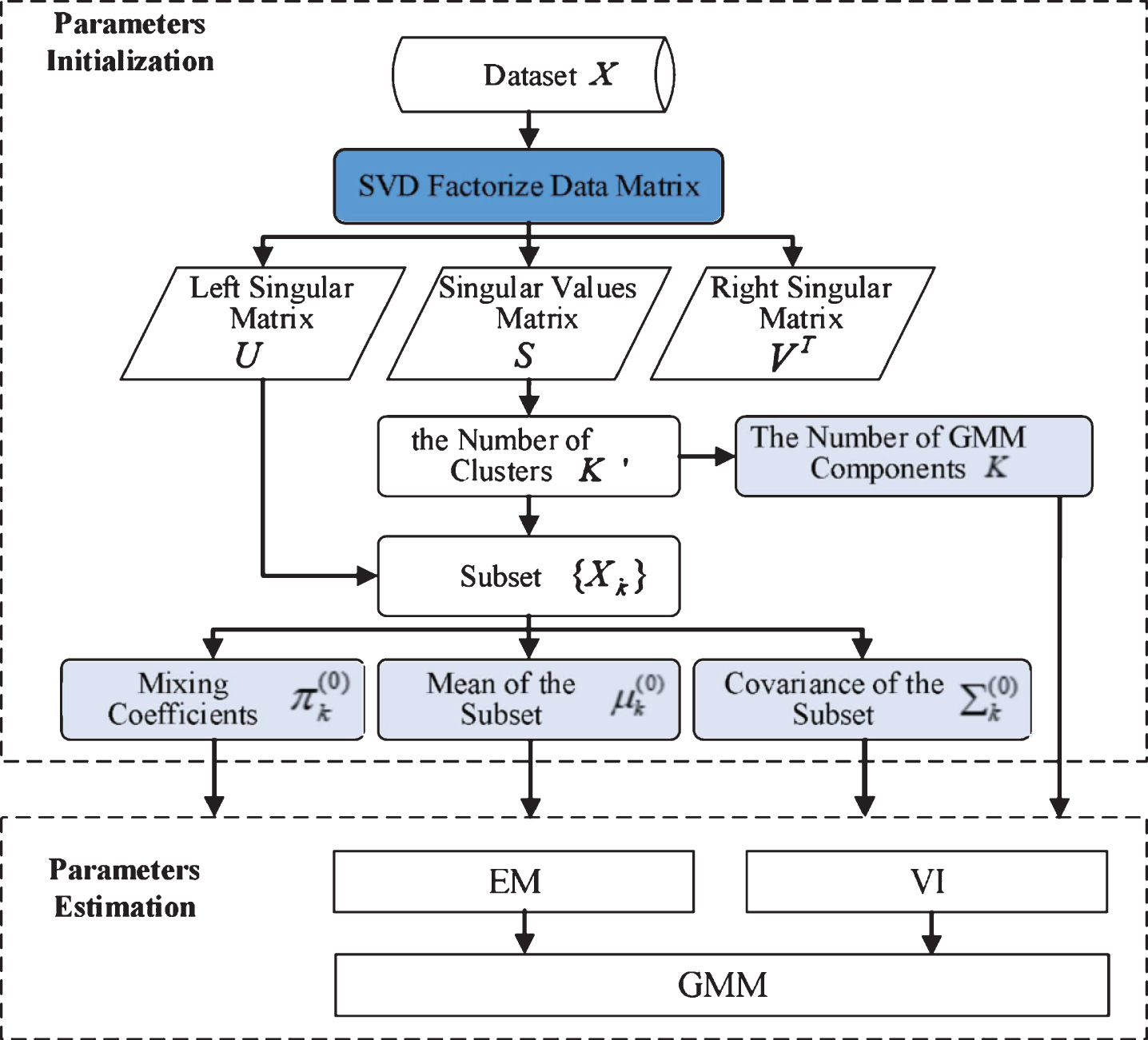
Overall solution of the model.

5 Experiments

In this section, to evaluate the performance of our proposed method, a series of experiments are arranged with respects of EM and VI algorithms in multivariate GMM starting with different initialization methods. The objective is to illustrate the performance of our method by comparing with different other methods working on different data sets.

5.1 Experimental data sets and Settings

In this paper, our goal is to evaluate our proposed method to initialize parameters in Gaussian mixture clustering models to analyze network security data to find the hidden threat behavior. To illustrate our proposed method works helpful, we get some public security data sets and UCI common data sets with different dimensions and clusters. We investigate the performance of five different initialization methods: RndEM [27], ∑-EM [13], K-means (denoted as KmEM), Random method and our proposed method (denoted as SVD-based). And we use the Adjusted Rand Index(ARI) to evaluate the performance of the experiments. All experiments are preformed in JetBrains PyCharm 2017 with python 3.6 interpreter on a laptop Intel CORE i5-6200U 2.3 GHz with 8GB RAM running the Windows 10 OS.

5.1.1 Data sets

In this section, we introduce the data sets containing the security data sets and common data sets from UCI machine learning repository [50]. The details of the data sets are presented in Table 1.

Table 1
The details of the data sets used ins the experiments

Data sets(X) Sample Sizes (N) Attribute Dimensions (D) Original Clusters or the Length of True Labels (K₀) Sample Distribution Overlap Degree (Silhouette Coefficient) Attribute Types

Spambase.csv 4601 57 2 2788/1813 0.992 Integer, Real

Phishing Websites.csv 11055 30 2 6157/4898 0.235 Binary

Websites Phishing.csv 1353 9 3 548/103 0.225 Binary

KDDCUP 10percent Multiclass.csv 494021 41 5 97278/391458/410 0.999 Integer, Real

7/1126/52

KDDCUP 10percent 2class.csv 494021 41 2 396743/97278 0.999 Integer, Real

Iris.csv 150 4 3 50/50/50 0.546 Real

Wine.csv 440 7 3 59/71/48 0.424 Integer, Real

Data sets(X)	Sample Sizes (N)	Attribute Dimensions (D)	Original Clusters or the Length of True Labels (K₀)	Sample Distribution	Overlap Degree (Silhouette Coefficient)	Attribute Types
Spambase.csv	4601	57	2	2788/1813	0.992	Integer, Real
Phishing Websites.csv	11055	30	2	6157/4898	0.235	Binary
Websites Phishing.csv	1353	9	3	548/103	0.225	Binary
KDDCUP 10percent Multiclass.csv	494021	41	5	97278/391458/410	0.999	Integer, Real
				7/1126/52
KDDCUP 10percent 2class.csv	494021	41	2	396743/97278	0.999	Integer, Real
Iris.csv	150	4	3	50/50/50	0.546	Real
Wine.csv	440	7	3	59/71/48	0.424	Integer, Real

In Table 1, there are 7 data sets containing 5 security data sets in first five and 2 common databases from UCI machine learning repository in last two. These data sets have their own characteristics. Firstly, the data sets have different sample sizes, attribute dimensions and the number of the original clusters. Among them, KDDCUP 10percent Multiclass.csv and KDDCUP 10percent 2class.csv are the biggest data sets with big sample size. Secondly, the data sets have different sample distribution, Spambase.csv, Phishing Websites.csv, Iris.csv and Wine.csv are balanced data sets, while Websites Phishing.csv, KDDCUP 10percent Multiclass.csv and KDDCUP 10percent 2class.csv are unbalanced data sets. In unbalanced data sets, the minority examples are more likely to be misclassified. Thirdly, the data sets have different overlap degree, which is measured by silhouette coefficient. The silhouette coefficient score is bounded between -1 for incorrect clustering and +1 for highly dense clustering. When the core around zero indicates the clusters is overlapping. Among all the data sets, KDDCUP 10percent Multiclass.csv, KDDCUP 10percent 2class.csv and Spambase.csv have lower overlap degree, while Phishing Websites.csv and Websites Phishing.csv have higher overlap degree. Fourthly, the data sets have different attribute types. The attribute types of Spambase.csv, KDDCUP 10percent Multiclass.csv, KDDCUP 10percent 2class.csv and Wine.csv are integer and real. The attribute types of Phishing Websites.csv and Websites Phishing.csv are binary. The attribute type of Iris.csv is real. These differences in data sets lead to different performance of GMM models.

5.1.2 Baseline approaches

We compare our methods with the following baseline approaches:

RndEM [27] is a staged approach to specify initial values by finding a large number of local modes. This method valuates the likelihood at the initial valid random start and chooses the parameters with highest likelihood.

∑-EM [13] is proposed to initialize EM algorithm to determine the number of GMM components. The method finds initial parameter by choosing samples with higher concentrations of neighbors to form clusters and then eliminates the fake components by comparing the Bayesian Information Criterion (BIC).

KmEM [29, 51] can divide data sets into Kclusters through assigning each sample to the nearest cluster center. KmEM is conceptual simplicity and computational scalability, so it is widely used as a initialization method to separate samples into different groups at first step and it can quickly provide a reasonable single-membership partition as a starting sample for GMM inference.

RndEM, ∑-EM and KmEM have already used as initiation methods for EM. While there are few literatures to study the initiation method for VI. So we can only compare our proposed method with the approaches for EM. Actually, both our proposed method and the baseline approaches are working in the stage before EM and VI estimating parameters. Therefore, the baseline approaches are very suitable for comparison.

5.1.3 Evaluation metrics

In this paper, we use the ARI to evaluate the all experiment results which are shown in section 5.2. ARI computers the similarity between two clusters by computing all pairs numbers of samples, and the pairs that are assigned in the same or different clusters according to the true cluster labels and the predicted cluster labels [13, 52]. The range of the ARI values is [–1, 1]. When the ARI values are negative indicating the clustering results are bad and the predicted labels are independent. On the contrary, When the ARI values are close to 1 indicating the clustering result is a perfect match between the true labels and predicted labels. The advantage of ARI is that it does not make any assumption on the cluster structure and it can be used to compare the similarities between clustering results of any clustering algorithm. But ARI needs to know the true labels. The ARI is defined as follows: $ARI = \frac{RI - E [RI]}{max (RI) - E [RI]}$ (29) $RI = \frac{n_{1} + n_{2}}{C_{2}^{n}}$ (30) where $C_{2}^{n}$ is the total number of possible pairs of samples in the data sets without ordering. n₁ is the number of pairs of samples which are in the same cluster with the true labels and the predicted labels. n₂ is the number of pairs of samples which are in different clusters in the true labels and in the predicted labels.

5.2 Experimental results

5.2.1 Evaluation on the number of GMM components based on SVD

In GMM, the number of mixing components K is important, which determines the final clustering results. In this section, we use our proposed method to obtain the initia value of K. Firstly, we use SVD to factorize the data matrix to divide the data into K initial clusters which is equivalent to the mixing components of the probabilistic model. Secondly, the mixing coefficients π_k of each component is set to 1/K, the mean μ_k of each component is set to equal the mean of X, and the convariance ∑_k of each component is set to equal the covariance of X. Thirdly, we input these initial values into GMM, then the parameters are further estimated by EM and VI respectively. To illustrate the effectiveness of the proposed method, we manually set K to the fixed numbers in the range [2, 10]. By comparing the performance of GMM with initial value based on SVD and fixed value, we can find our initialization algorithm computing K value based on SVD is appropriate. The number of model iteration is performed to 100. The performance of GMM clustering using EM and VI estimating parameters initialized based on the fixed values setting and SVD is summarized in Tables 2 and 3.

Table 2
Summarized Adjusted Rand Index (ARI) and the components number of GMM clustering using EM estimating parameters with fixed values setting and SVD-based initialization methods

data set Fixed Values Setting of the Components Number SVD-based

K = 2 K = 3 K = 4 K = 5 K = 6 K = 7 K = 8 K = 9 K = 10

Spambase.csv 0.183 0.203 0.223 0.233 0.193 0.174 0.252 0.128 0.132 K = 5

ARI = 0.233

Phishing Websites.csv 0.122 0.126 0.428 0.086 0.154 0.034 0.136 0.164 0.180 K = 3

ARI = 0.126

Websites Phishing.csv 0.512 0.209 0.057 0.154 0.087 0.142 0.107 0.127 0.100 K = 2

ARI = 0.512

KDDCUP 10percent Multiclass.csv 0.214 0.272 0.376 0.382 0.372 0.442 0.443 0.446 0.440 K = 13

ARI = 0.436

KDDCUP 10percent 2class.csv 0.202 0.357 0.358 0.358 0.352 0.424 0.420 0.419 0.360 K = 13

ARI = 0.451

Iris.csv 0.568 0.644 0.601 0.512 0.507 0.534 0.601 0.552 0.562 K = 3

ARI = 0.644

Wine.csv 0.453 0.582 0.405 0.402 0.367 0.371 0.338 0.319 0.216 K = 3

ARI = 0.582

data set	Fixed Values Setting of the Components Number	SVD-based
Spambase.csv	0.183	0.203	0.223	0.233	0.193	0.174	0.252	0.128	0.132	K = 5
										ARI = 0.233
Phishing Websites.csv	0.122	0.126	0.428	0.086	0.154	0.034	0.136	0.164	0.180	K = 3
										ARI = 0.126
Websites Phishing.csv	0.512	0.209	0.057	0.154	0.087	0.142	0.107	0.127	0.100	K = 2
										ARI = 0.512
KDDCUP 10percent Multiclass.csv	0.214	0.272	0.376	0.382	0.372	0.442	0.443	0.446	0.440	K = 13
										ARI = 0.436
KDDCUP 10percent 2class.csv	0.202	0.357	0.358	0.358	0.352	0.424	0.420	0.419	0.360	K = 13
										ARI = 0.451
Iris.csv	0.568	0.644	0.601	0.512	0.507	0.534	0.601	0.552	0.562	K = 3
										ARI = 0.644
Wine.csv	0.453	0.582	0.405	0.402	0.367	0.371	0.338	0.319	0.216	K = 3
										ARI = 0.582

Table 3

Summarized Adjusted Rand Index (ARI) and the components number of GMM clustering using VI estimating parameters with fixed values setting and SVD-based initialization methods

data set	Fixed Values Setting of the Components Number									SVD-based
	K = 2	K = 3	K = 4	K = 5	K = 6	K = 7	K = 8	K = 9	K = 10
Spambase.csv	0.228	0.234	0.233	0.245	0.196	0.215	0.283	0.238	0.112	K = 5
										ARI = 0.245
Phishing Websites.csv	0.142	0.288	0.333	0.343	0.197	0.144	0.280	0.110	0.158	K = 3
										ARI = 0.288
Websites Phishing.csv	0.510	0.229	0.269	0.186	0.224	0.130	0.179	0.125	0.107	K = 2
										ARI = 0.510
KDDCUP 10percent Multiclass.csv	0.0001	0.0009	0.0013	0.462	0.462	0.677	0.735	0.751	0.748	K = 13
										ARI = 0.744
KDDCUP 10percent 2class.csv	–0.0003	–0.0001	–0.0002	0.0002	0.478	0.710	0.717	0.730	0.713	K = 13
										ARI = 0.728
Iris.csv	0.568	0.904	0.786	0.767	0.519	0.514	0.442	0.412	0.415	K = 3
										ARI = 0.904
Wine.csv	0.310	0.607	0.381	0.306	0.338	0.244	0.241	0.181	0.169	K = 3
										ARI = 0.607

Tables 2 and 3 summarize the ARI and the components number of GMM clustering using EM and VI estimating parameters with fixed values setting and SVD-based initialization methods, respectively. Firstly, we fix the range of the components number is [2, 10], and calculate the ARI of GMM. Then we calculate the components number based on SVD and the ARI of GMM.

From the experiment results, we find that, in most cases, the numbers of components corresponding to the best ARI in the fixed range and the numbers of components based on SVD are not the same. And theyare not equal to the original numbers of the clusters in Table 1. Furthermore, in most cases, the ARIs based on SVD are better than that of the original clusters, and close to the highest ARIs in the fixed range. However, comparing the best the components numbers and ARIs through the numerous attempts in the fixed range like BIC, our SVD-based method only executes once to get better results. For Websites Phishing.csv, Iris.csv and Wine.csv, our SVD-based method receive the best performance, which is the same to that of the original clusters. Therefore, our proposed approach is recommended for the numbers of components initialization. Comparing the ARI of the same data sets and the numbers of components in Tables 2 and 3, we find VI is better than EM on the parameter estimating for GMM clustering. Especially on the big data sets, such as KDDCUP 10percent Multiclass.csv and KDDCUP 10percent 2class.csv, the performance is greatly improved by VI. Maybe it is easy for EM to fall into the local optimum in the iterative process. However, the efficiency of VI is lower than that of EM in the whole process, especially on the big data sets. This can be explained by the complexity of the algorithms, where the steps of VI are more complicated than that of EM according to the formulas (12)-(24) and (4)-(6). Therefore, if the performance is the final target, VI is recommended for the optimal parameter estimating.

5.2.2 Comparison initialization values by SVD-based and fixed values

In last section, through comparing the performance of the components initial number K based on fixed values with a range [2, 10] _{andSVD - based}, we find that the component initial number K based on SVD can provide preferable effect. In this section, we want to prove the initialization values of the mixing coefficients π_k, the mean μ_k and the convariance ∑_k based on SVD are useful to improve the performance of GMM, comparing the fixed initialization values. For the initialization values based on SVD, the values of K are calculated by the first two singular values and the dimension of D, the values of the mixing coefficients π_k, the mean μ_k and the convariance ∑_k are calculated based on K. As the comparative algorithm, the parameters values are all initialized to the fixed value, such as the components number K is set to equal the length of true labels K₀, the mixing coefficients π_k of each component is set to 1/K, the mean μ_k of each component is set to equal the mean of X, and the convariance ∑_k of each component is set to equal the covariance of X. The number of model iterations is performed to 100. All parameters initialized based on SVD and the fixed values of GMM clustering using EM is summarized in Tables 4 and 5.

Table 4
Summarized the performance of all parameters initialized based on SVD and the fixed values of GMM clustering using EM

data set K initialized by SVD-based All parameters initialized by SVD-based Fixed method

K _ARI K _ARI K _ARI

Spambase.csv 5 0.233 5 0.251 2 0.183

Phishing Websites.csv 3 0.126 3 0.178 2 0.122

Websites Phishing.csv 2 0.512 2 0.553 3 0.209

KDDCUP 10percent Multiclass.csv 13 0.436 13 0.449 5 0.382

KDDCUP 10percent 2class.csv 13 0.451 13 0.450 2 0.202

Iris.csv 3 0.644 3 0.667 3 0.644

Wine.csv 3 0.582 3 0.601 3 0.582

data set	K initialized by SVD-based	All parameters initialized by SVD-based	Fixed method
Spambase.csv	5	0.233	5	0.251	2	0.183
Phishing Websites.csv	3	0.126	3	0.178	2	0.122
Websites Phishing.csv	2	0.512	2	0.553	3	0.209
KDDCUP 10percent Multiclass.csv	13	0.436	13	0.449	5	0.382
KDDCUP 10percent 2class.csv	13	0.451	13	0.450	2	0.202
Iris.csv	3	0.644	3	0.667	3	0.644
Wine.csv	3	0.582	3	0.601	3	0.582

Table 5

Summarized the performance of all parameters initialized based on SVD and the fixed values of GMM clustering using VI

data set	K initialized by SVD-based		All parameters initialized by SVD-based		Fixed method
	K	_ARI	K	_ARI	K	_ARI
Spambase.csv	5	0.245	5	0.326	2	0.228
Phishing Websites.csv	3	0.333	3	0.481	2	0.142
Websites Phishing.csv	2	0.510	2	0.582	3	0.229
KDDCUP 10percent Multiclass.csv	13	0.744	13	0.753	5	0.462
KDDCUP 10percent 2class.csv	13	0.728	13	0.718	2	–0.0003
Iris.csv	3	0.904	3	0.908	3	0.904
Wine.csv	3	0.607	3	0.637	2	0.607

Tables 4 and 5 summarize the ARI and the components number of GMM clustering using EM and VI estimating optimal parameters with K initialized and all parameters initialized by SVD-based method and fixed method, respectively. Firstly, we calculate the components number K based on SVD and the ARI of GMM while other parameters initialized on the fixed values. Secondly, we calculate all parameters initialized based on SVD and the ARI of GMM. Thirdly, we calculate the ARI of GMM when all parameters initialized on the fixed values. From the experiment results in Tables 4 and 5, we find that, in most cases, the performance of all parameters initialized based on SVD is better than that of only K initialized based on SVD. Meanwhile, the performance of all parameters initialized based on SVD is far better than that of all parameters with fixed values. In addition, comparing the results between Tables 4 and 5, we find the performance of VI is better than that of EM on the parameter estimating for GMM clustering.

5.2.3 Comparison initialization methods by SVD-based and other deterministic methods

In the existing literatures, there already have been some deterministic initialization methods, such as RndEM, ∑-EM and KmEM. In this section, we compare our initialization methods by SVD-based and other deterministic methods. In SVD-based initialization method, the values of the parameters are calculated based on the matrix decomposition of the original data set. In RndEM, ∑-EM and KmEM, the components number K is calculated according to the steps of the algorithms, respectively. And then the initialization values of the mixing coefficients π_k, the mean μ_k and the convariance ∑_k are calculated based on K. The number of model iterations is performed to 100. The performance of GMM clustering using EM and VI initialized based on different methods is summarized in Tables 6 and 7

Table 6
Summarized the performance of all parameters initialized based on different methods of GMM clustering using EM

data set RndEM ∑-EM KmEM SVD-based

K _ARI K _ARI K _ARI K _ARI

Spambase.csv ₂ _0.218 ₂ _0.206 2 _0.235 5 0.251

Phishing Websites.csv ₂ _0.135 ₃ _0.176 2 _0.141 3 0.178

Websites Phishing.csv ₃ _0.208 ₂ _0.294 3 _0.259 2 0.553

KDDCUP 10percent Multiclass.csv _– _– _– _– 5 _0.399 13 0.449

KDDCUP 10percent 2class.csv _– _– _– _– 2 _0.227 13 0.450

Iris.csv ₃ _0.574 ₂ _0.578 3 _0.649 3 0.667

Wine.csv ₃ _0.556 ₃ _0.510 3 _0.488 3 0.601

data set	RndEM	∑-EM	KmEM	SVD-based
Spambase.csv	₂	_0.218	₂	_0.206	2	_0.235	5	0.251
Phishing Websites.csv	₂	_0.135	₃	_0.176	2	_0.141	3	0.178
Websites Phishing.csv	₃	_0.208	₂	_0.294	3	_0.259	2	0.553
KDDCUP 10percent Multiclass.csv	_–	_–	_–	_–	5	_0.399	13	0.449
KDDCUP 10percent 2class.csv	_–	_–	_–	_–	2	_0.227	13	0.450
Iris.csv	₃	_0.574	₂	_0.578	3	_0.649	3	0.667
Wine.csv	₃	_0.556	₃	_0.510	3	_0.488	3	0.601

Table 7

Summarized the performance of all parameters initialized based on different methods of GMM clustering using VI

data set	RndEM		∑-EM		KmEM		SVD-based
	K	_ARI	K	_ARI	K	_ARI	K	_ARI
Spambase.csv	₂	_0.306	₂	_0.249	2	_0.267	5	0.326
Phishing Websites.csv	₂	_0.362	₃	_0.402	2	_0.214	3	0.481
Websites Phishing.csv	₃	_0.501	₂	_0.522	3	_0.312	2	0.582
KDDCUP 10percent Multiclass.csv	_–	_–	_–	_–	5	_0.457	13	0.753
KDDCUP 10percent 2class.csv	_–	_–	_–	_–	2	_–0.0003	13	0.718
Iris.csv	₃	_0.476	₂	_0.580	3	_0.568	3	0.912
Wine.csv	₃	_0.474	₃	_0.591	3	_0.519	3	0.637

Tables 6 and 7 summarize the ARI and the components number of GMM clustering using EM and VI estimating all parameters based on different methods, respectively. RndEM, ∑-EM and SVD-based methods calculate the components number K according to the theory. In KmEM, the initialized values of K come from the length of true labels K₀. From the experiment results in Tables 6 and 7, we find that, in most cases, SVD-based method prefers over other methods. The performance of KmEM is the worst on the security data set. And RndEM comes the next. ∑-EM and RndEM show similar results on the components number K_, while the ARI of ∑-EM is better than that of RndEM. Moreover, we can not use RndEM, ∑-EM to calculate the components number and the final ARI successfully on the big data, such as KDDCUP 10percent Multiclass.csv and KDDCUP 10percent 2class.csv. In the algorithmic program, we upload the whole data set into the memory at one time. Then the program calculate the Euclidean Distance between any two samples. When the amount of data is large, there is a memory overflow problem happening. To solve this problem, we will change the way to the algorithmic program. However, RndEM and ∑-EM have another obvious drawback that is the calculation process complicated, spending high source and taking long time. In conclusion, SVD-based method demonstrates good overall performance on all the parameters initialization, and performs well no matter how large the amount of data is and what the type of data is. Therefore, SVD-based is recommended as an excellent initialization method.

5.2.4 Computational complexity and running time

This section compares the computational cost of the initialization methods. We analyze the computational complexity based on the execution time of the algorithmic program, which is related to the number of iterations of some basic statements in the algorithm. The more iterations, the more time the method takes. In this section, we assume that the number of iterations of the algorithm is s, the number of samples is N, the dimension is D, and the number of clusters is K. The theoretical value of the computational complexity is analyzed in Table 8, where the execution time of the algorithm increases with the increase of the data size. Furthermore, we record the actual values of the computational complexity when the algorithmic programs are running. The actual values of the computational complexity is record in Table 9.

Table 8
Summarized the computational complexity of different initialization methods

Methods RndEM ∑-EM KmEM SVD-based

Complexity O^(N² D) O (N³ + N²^D) O (sNDK) O (D³)

Methods	RndEM	∑-EM	KmEM	SVD-based
Complexity	O^(N² *D)	O (N³ + N²^*D)	O (sNDK)	O (D³)

Table 9

Summarized the running time of the initialization methods

Methods	RndEM	∑-EM	KmEM	SVD-based
Spambase.csv	2.4076	322.5957	0.7281	0.3650
Phishing Websites.csv	8.9500	3113.7797	0.9853	0.5945
Websites Phishing.csv	0.1715	23.5620	0.0638	0.0697
KDDCUP 10percent Multiclass.csv	–	–	86.1527	57.7237
KDDCUP 10percent 2class.csv	–	–	87.8173	54.6863
Iris.csv	0.1176	1.1200	0.0309	0.0398
Wine.csv	0.4293	2.1981	0.0608	0.0299

Table 8 summarizes the computational complexity of different initialization methods. We find that the computational complexity is relate to the dimension and the number of the samples. When the dimension of the samples is higher than the number, the complexity of the SVD-based method is greatest. However, this case is rare in big data analysis. In actually, the number of the samples is far bigger than the dimension, and the complexity of the SVD-based method is lowest. By contrast, the complexity of ∑-EM is greatest, RndEM takes the second place, and KmEM takes the third place, whose complexity is less than that of SVD-based method.

Table 8 records the actual running time of different initialization methods. We find that SVD-based method cost the least time, KmEM cost less time, RndEM cost more time, and ∑-EM cost the most time. The results in Table 8 are consistent with those in Table 9. Therefore, we can conclude that SVD-based method outperforms other initialization methods in the computational complexity and running time.

6 Conclusion and future work

EM and VI are important for parameter estimation in GMM. Initialization is a crucial step in EM and VI that is because initialization can determine the convergence of the mixture models to the local maximum and also affect the speed of convergence. Presently, there already have been some initialization strategy for EM. However, no one outperforms other methods. Meanwhile, the majority of existing methods perform well on the simulate data but does not experience experiments on the real data sets. And the majority of existing methods have high complexity on the big data especially when deal with a large number of clusters.

Our proposed strategy is based on SVD to factorize the data set matrix to get the singular value matrix and singular matrixs. Then we calculate the number of the components of GMM by the first two singular values in the singular value matrix and the dimension of the data. Next, other parameters of GMM, such as the mixing coefficients,the mean and the convariance, are calculated based on the number of the components. The performance of GMM clustering using EM and VI estimating optimal parameters based on SVD initialization parameters is compared to three other initialization approaches on the security databases and common databases from UCI machine learning repository, which have different clusters, dimensions and types. However, SVD has some defects. For example, when the dimension of the data set is very high, the calculation complexity will be high. And when the data set matrix is too sparse, the effect of matrix decomposition is poor. Therefor, our proposed strategy can not deal with high dimension and sparse data set well.

The experiment results indicate that our proposed method performs well on the components number of GMM clustering using EM and VI estimating optimal parameters, and also other parameters containing the mixing coefficients, the mean and the convariance. And VI is better than EM on the optimal parameter estimating for GMM clustering. Especially on the big data set. Furthermore, our proposed method has good performance no matter how large the amount of data is and what the type of data is. Therefore, our proposed approach is recommended for the parameters initialization of the EM and VI optimal parameter estimation in GMM.

Footnotes

Acknowledgments

The author would like to thank the editor and the referees for their helpful suggestions and comments that considerably improved this paper. This paper is based upon the work supported by National Natural Science Foundation of Zhejiang Province (LY20F020012, LQ19F020008), National Natural Science Foundation of China (61802094, 61272539, 72002133), Ministry of Education of China Science Foundation (19YJC630174), China Postdoctoral Science Foundation (2018M630461), Natural Science Foundation of Beijing Municipality (4194076).

References

Fan

, Bouguila

and Sallay

, Anomaly intrusion detection using incremental learning of an infinite mixture model with feature selection, International Conference on Rough Sets and Knowledge Technology. Springer, Berlin, Heidelberg, 2013.

Tsai

C.F.

, Hsu

Y.F.

and Lin

C.Y.

, et al., Intrusion detection by machine learning: A review, Expert Systems with Applications 36(10) (2009), 11994–12000.

Mayhew

, Atighetchi

and Adler

, et al., Use of machine learning in big data analytics for insider threat detection, MILCOM 2015-2015 IEEE Military Communications Conference, IEEE, (2015), 915–922.

Agrawal

and Agrawal

, Survey on anomaly detection using data mining techniques, Procedia Computer Science 60 (2015), 708–713.

Nicholas

, Ooi

S.Y.

, Pang

Y.H.

, Hwang

S.O.

and Tan

S.Y.

, Study of long short-term memory in flow-based network intrusion detection system, Journal of Intelligent & Fuzzy Systems 35(6) (2018), 5947–5957.

O’Hagan

and White

, Improved model-based clustering performance using Bayesian initialization averaging, Computational Statistics 34(1) (2019), 201–231.

Chen

, An effective synchronization clustering algorithm, Applied Intelligence 46(1) (2017), 135–157.

Nguyen

H.L.

, Woon

Y.K.

and Ng

W.K.

, A survey on data stream clustering and classification, Knowledge and Information Systems 45(3) (2015), 535–569.

Chen

, Qian

and Wang

, et al., Large-scale fuzzy multiple-medoid clustering method, Journal of Intelligent and Fuzzy Systems 32(3) (2017), 1833–1845.

10.

Biernacki

and Celeux

, and G Govaert, Choosing starting values for the EM algorithm for getting the highest likelihood in multivariate Gaussian mixture models, Computational Statistics and Data Analysis 41(3-4) (2003), 561–575.

11.

Bagherinia

, Minaei-Bidgoli

and Hossinzadeh

, et al., Elite fuzzy clustering ensemble based on clustering diversity and quality measures, Applied Intelligence 49(5) (2019), 1724–1747.

12.

Bouveyron

, Girard

and Schmid

, High-dimensional data clustering, Computational Statistics and Data Analysis 52(1) (2007), 502–519.

13.

Melnykov

and Melnykov

, Initializing the EM algorithm in Gaussian mixture models with an unknown number of components, Computational Statistics and Data Analysis 56(6) (2012), 1381–1395.

14.

Melnykov

and Maitra

, Finite mixture models and model-based clustering, Statistics Surveys 4 (2010), 80–116.

15.

Zong

, Song

and Min

M.R.

, et al, Deep autoencoding gaussian mixture model for unsupervised anomaly detection, 2018.

16.

and Leijon

, Bayesian estimation of beta mixture models with variational inference, IEEE Transactions on Pattern Analysis and Machine Intelligence 33(11) (2011), 2160–2173.

17.

Nguyen

T.M.

, Wu

Q.M.J.

and Zhang

, Bounded generalized Gaussian mixture model, Pattern Recognition 47(9) (2014), 3132–3142.

18.

, Fan

and Du

J.X.

, et al., A novel statistical approach for clustering positive data based on finite inverted Beta-Liouville mixture models, Neurocomputing 333 (2019), 110–123.

19.

Yao

and Ge

, Scalable Semisupervised GMM for Big Data Quality Prediction in Multimode Processes, IEEE Transactions on Industrial Electronics 66(5) (2018), 3681–3692.

20.

, Lai

and Kleijn

B.W.

, et al., Variational Bayesian learning for Dirichlet process mixture of inverted Dirichlet distributions in non-Gaussian image feature modeling, IEEE Transactions on Neural Networks and Learning Systems 30(2) (2018), 449–463.

21.

Lai

, Ma

and Xu

, et al., Positive Data Modeling Using a Mixture of Mixtures of Inverted Beta Distributions, IEEE Access 7 (2019), 38146–38156.

22.

Fan

, Al-Osaimi

F.R.

and Bouguila

, et al., Proportional data modeling via entropy-based variational bayes learning of mixture models, Applied Intelligence 47(2) (2017), 473–487.

23.

Yang

M.S.

, Lai

C.Y.

and Lin

C.Y.

, A robust EM clustering algorithm for Gaussian mixture models, Pattern Recognition 45(11) (2012), 3950–3961.

24.

and Dy

J.G.

, In search of deterministic methods for initializing K-means and Gaussian mixture clustering, Intelligent Data Analysis 11(4) (2007), 319–338.

25.

Denisova

and Sergeyev

, Using hierarchical histogram representation for the EM clustering algorithm enhancement, Proceedings of the 10th International Symposium on Image and Signal Processing and Analysis. IEEE, (2017), 41–46.

26.

Nasios

and Bors

A.G.

, Variational learning for Gaussian mixture models, IEEE Transactions on Systems, Man, and Cybernetics, Part B (Cybernetics) 36(4) (2006), 849–862.

27.

Maitra

, Initializing partition-optimization algorithms, IEEE/ACM Transactions on Computational Biology and Bioinformatics 6(1) (2009), 144–157.

28.

Fraley

and Raftery

A.E.

, Model-based clustering, discriminant analysis, and density estimation, Journal of the American Statistical Association 97(458) (2002), 611–631.

29.

Wan

, Liu

and Wu

, et al., ICGT: A novel incremental clustering approach based on GMM tree, Data & Knowledge Engineering 117 (2018), 71–86.

30.

Maitra

and Melnykov

, Simulating data to study performance of finite mixture modeling and clustering algorithms, Journal of Computational and Graphical Statistics 19(2) (2010), 354–376.

31.

Karlis

and Xekalaki

, Choosing initial values for the EM algorithm for finite mixtures, Computational Statistics and Data Analysis 41(3-4) (2003), 577–590.

32.

Boutsidis

and Gallopoulos

, SVD based initialization: A head start for nonnegative matrix factorization, Pattern Recognition 41(4) (2008), 1350–1362.

33.

Becker

J.M.

and Menzel

, Rohlfing

, Complex SVD initialization for NMF source separation on audio spectrograms, DAGA, 2015.

34.

Zong

, Song

and Min

M.R.

, et al. Deep autoencoding gaussian mixture model for unsupervised anomaly detection. 2018.

35.

Gaussian mixture models, https://scikit-learn.org/stable/modules/mixture.html#mixture.

36.

Bonilla

E.V.

, Chai

K.M.

and Williams

, Multi-task Gaussian process prediction, Advances in Neural Information Processing systems, (2008), 153–160.

37.

McLachlan

and Peel

, Finite mixture models, John Wiley and Sons, USA, 2004. https://www-tandfonline-com-s.web.bisu.edu.cn/doi/abs/10.1198/tech.2002.s651

38.

Bishop

C.M.

, Pattern recognition and machine learning, Springer, Berlin, 2006.

39.

, Taghia

and Guo

, On the Convergence of ExtendedVariational Inference for Non-Gaussian Statistical Models, arXiv preprint arXiv:1902,05068, 2019.

40.

Blei

D.M.

and Jordan

M.I.

, Variational inference for Dirichlet process mixtures, Bayesian Analysis 1(1) (2006), 121–143.

41.

Attias

, A variational baysian framework for graphical models, Advances in Neural Information Processing Systems, (2000), 209–215.

42.

Fan

, Sallay

and Bouguila

, et al., Variational learning of hierarchical infinite generalized Dirichlet mixture models and applications, Soft Computing 20(3) (2016), 979–990.

43.

Lim

Y.J.

and Teh

Y.W.

, Variational Bayesian approach to movie rating prediction, Proceedings of KDD cup and workshop 7 (2007), 15–21.

44.

Tzikas

D.G.

, Likas

A.C.

and Galatsanos

N.P.

, The variational approximation for Bayesian inference, IEEE Signal Processing Magazine 25(6) (2008), 131–146.

45.

Choudrey

R.A.

and Roberts

S.J.

, Variational mixture of Bayesian independent component analyzers, Neural Computation 15(1) (2003), 213–252.

46.

Peña

J.M.

and Sauer

, SVD update methods for large matrices and applications, Linear Algebra and its Applications 561 (2019), 41–62.

47.

Qiao

, New SVD based initialization strategy for non-negative matrix factorization, Pattern Recognition Letters 63 (2015), 71–77.

48.

Zhao

and Ye

, Singular value decomposition packet and its application to extraction of weak fault feature, Mechanical Systems and Signal Processing 70 (2016), 73–86.

49.

Kim

, Sparse inverse covariance learning of conditional Gaussian mixtures for multiple output regression, Applied Intelligence 44(1) (2016), 17–29.

50.

UCI Machine Learning Repository, http://archive.ics.uci.edu/ml/datasets.php.

51.

Raykov

Y.P.

, Boukouvalas

and Baig

, et al., What to do when k-means clustering fails: A simple yet principled alternative algorithm, PloS One 1(9) (2016), 1e0162259.

52.

Clustering performance evaluation, https://scikit-learn.org/stable/modules/clustering.html#clustering-evaluation.

GMM with parameters initialization based on SVD for network threat detection

Abstract

Keywords

1 Introduction

2 GMM and parameters inference

2.1 GMM

5.1 Experimental data sets and Settings

5.1.1 Data sets

5.1.3 Evaluation metrics

5.2.1 Evaluation on the number of GMM components based on SVD

Table 8 Summarized the computational complexity of different initialization methods Methods RndEM ∑-EM KmEM SVD-based Complexity O(N2 *D) O (N3 + N2*D) O (sNDK) O (D3)

Footnotes

Acknowledgments

References

Table 8
Summarized the computational complexity of different initialization methods

Methods RndEM ∑-EM KmEM SVD-based

Complexity O^(N² D) O (N³ + N²^D) O (sNDK) O (D³)