Certain efficient iterative methods for bipolar fuzzy system of linear equations

Abstract

A bipolar fuzzy set model is an extension of fuzzy set model. We develop new iterative methods: generalized Jacobi, generalized Gauss-Seidel, refined Jacobi, refined Gauss-seidel, refined generalized Jacobi and refined generalized Gauss-seidel methods, for solving bipolar fuzzy system of linear equations(BFSLEs). We decompose n × n BFSLEs into 4n × 4n symmetric crisp linear system. We present some results that give the convergence of proposed iterative methods. We solve some BFSLEs to check the validity, efficiency and stability of our proposed iterative schemes. Further, we compute Hausdorff distance between the exact solutions and approximate solution of our proposed schemes. The numerical examples show that some proposed methods converge for the BFSLEs, but Jacobi and Gauss-seidel iterative methods diverge for BFSLEs. Finally, comparison tables show the performance, validity and efficiency of our proposed iterative methods for BFSLEs.

Keywords

Bipolar fuzzy system of linear equations generalized Jacobi method generalized Gauss-sediel method refined generalized Jacobi method refined generalized Gauss-seidel method

1 Introduction

Linear systems of equations play a vital role in many real life problems such as optimization, finance, engineering and economics. There exist several linear systems in which the parameters are not defined in precise, that is, we have to deal with imprecision and uncertainty. These types of systems are known as fuzzy systems. Friedman et al. [20] studied a model to solve the fuzzy system of linear equations (FSLEs) by using the embedding technique introduced in [17]. Many uncertain linear systems have been discussed in [13]. Allahviranloo [10, 11] introduced Jacobi, Guass-Seidel and SOR methods for approximating the solution of FSLEs. Deghan and Hashemi [19] introduced several iterative methods for strictly diagonally dominant FSLEs having all positive diagonal entries. Abbasbandy et al. [1, 3] proposed and analyzed LU decomposition and conjugate gradient methods for FSLEs. Jafarian and Abbasbandy [2] introduced Steepest Descent method. Allahviranloo [12] applied adomian decomposition method to find iterative methods for FSLEs. Najafi et al. [23] proposed an iterative method for FSLEs based on homotopy perturbation method and made a comparison with the iterative methods introduced by Allahviranloo [12]. Allahviranloo et al. [15, 16] used 1-cut expansion and defined a new metric to derive some methods to obtain fuzzy symmetric solutions. Allahviranloo and Ghanbari [14] introduced an "interval inclusion linear system", to propose a new approach for the solution of FSLEs. Zhang [26, 27] extended the concept of fuzzy set to bipolar fuzzy set. A bipolar fuzzy set is powerful tool to deal with the problems having fuzziness and vagueness. This frame is more attractive for researchers as compared to fuzzy frame. A bipolar fuzzy has two parts, namely positive and negative part. The positive part indicate that what would be granted to be possible and negative part indicate that what would be considered to be impossible. Akram and Arshad [5] introduced a new method for group decision making. Recently, Akram et al. [7] extended the concept of fuzzy system of linear equation to bipolar fuzzy system of linear equations and also solve it for bipolar fully fuzzy linear system with (-1,1)-cut position.

In this paper, we convert n × n BFSLEs into 4n × 4n crisp linear system extending the concept of Friedman [20]. We introduce some iterative methods to approximate the solution of BFSLEs. We give some theorems related to the convergence of our proposed iterative methods. We solve some numerical examples of BFSLEs by using these iterative methods and make a comparison with the Jacobi and Gauss-seidel methods introduced in [6]. We give some definitions and results in section 2 which would be further used in this work. In section 3, we demonstrate our main iterative methods. In section 4, we give some theorems related to the convergence of our iterative methods. Some numerical examples have been given in section 5 to see the performance and accuracy of introduced methods. Lastly, we draw some conclusions in section 6.

2 Preliminaries

In this section, we give basic definitions and results which are used in this document.

Definition 2.1. [7] The parametric form of bipolar fuzzy number (BFN) u is a quadruple

$≺ [{\underline{u}}^{P}, {\bar{u}}^{P}], [{\underline{u}}^{N}, {\bar{u}}^{N}] ≻$ of the functions ${\underline{u}}^{P} (t)$ , ${\bar{u}}^{P} (t)$ , ${\underline{u}}^{N} (w)$ , ${\bar{u}}^{N} (w)$ ; 0 ≤ t ≤ 1, -1 ≤ w ≤ 0, which satisfy the following conditions:

${\underline{u}}^{P} (t)$ is a bounded, non-decreasing, right continuous at 0 and left continuous function on (0, 1].

${\bar{u}}^{P} (t)$ is a bounded, non-increasing, right continuous at 0 and left continuous function on (0, 1].

${\underline{u}}^{N} (w)$ is a bounded, non-increasing, right continuous at ’-1’ and left continuous function on (-1, 0].

${\bar{u}}^{N} (w)$ is a bounded, non-decreasing, right continuous at ’-1’ and left continuous function on (-1, 0].

${\underline{u}}^{P} (t) \leq {\bar{u}}^{P} (t)$ ,

${\underline{u}}^{N} (w) \leq {\bar{u}}^{N} (w)$ .

Definition 2.2. [7] For arbitrary $u = ≺ [\underline{u^{P}}, {\bar{u}}^{P}], [{\underline{u}}^{N}, {\bar{u}}^{N}] ≻$ , $v = ≺ [{\underline{v}}^{P}, {\bar{v}}^{P}], [{\underline{v}}^{N}, {\bar{v}}^{N}] ≻$ and c > o, we define (u + v), (u . v) and scalar multiplication by c as follows:

$(\underline{u^{P} + v^{P}}) (t) = {\underline{u}}^{P} (t) + {\underline{v}}^{P} (t)$ ,

$(\bar{u^{P} + v^{P}}) (t) =$ ${\bar{u}}^{P} (t) + {\bar{v}}^{P} (t)$ ,

$(\underline{u^{N} + v^{N}}) (w) = {\underline{u}}^{N} (w) + {\underline{v}}^{N} (w)$ ,

$(\bar{u^{N} + v^{N}})$ $(w) = {\bar{u}}^{N} (w) + {\bar{v}}^{N} (w)$ ,

${\underline{u^{P} v}}^{P} = min {{\underline{u}}^{P} {\underline{v}}^{P}, {\underline{u}}^{P} {\bar{v}}^{P}, {\bar{u}}^{P} {\underline{v}}^{P}, {\bar{u}}^{P} {\bar{v}}^{P}}$ ,

$\bar{u^{P} v^{P}} = max {{\underline{u}}^{P} {\underline{v}}^{P}, {\underline{u}}^{P} {\bar{v}}^{P}, {\bar{u}}^{P} {\underline{v}}^{P}, {\bar{u}}^{P} {\bar{v}}^{P}}$ ,

${\underline{u^{N} v}}^{N}$ = $max {{\underline{u}}^{N} {\underline{v}}^{N}, {\underline{u}}^{N} {\bar{v}}^{N}, {\bar{u}}^{N} {\underline{v}}^{N}, {\bar{u}}^{N} {\bar{v}}^{N}}$ ,

$\bar{u^{N} v^{N}}$ = $min {{\underline{u}}^{N} {\underline{v}}^{N}, {\underline{u}}^{N} {\bar{v}}^{N}, {\bar{u}}^{N} {\underline{v}}^{N}, {\bar{u}}^{N} {\bar{v}}^{N}}$ ,

$({\underline{cu}}^{P}) (t) = c ({\underline{u}}^{P}) (t)$ , $({\bar{cu}}^{P}) (t) = c ({\bar{u}}^{P}) (t)$ ,

$({\underline{cu}}^{N}) (w)$ = $c ({\underline{u}}^{N}) (w)$ , $({\bar{cu}}^{N}) (w)$ = $c ({\bar{u}}^{N}) (w)$ .

Definition 2.3. [7] The n × n linear system of‘ equations $\begin{matrix} b_{11} y_{1} + b_{12} y_{2} + b_{13} y_{3} + \dots + b_{1 n} y_{n} & = z_{1}, \\ b_{21} y_{1} + b_{22} y_{2} + b_{23} y_{3} + \dots + b_{2 n} y_{n} & = z_{2}, \\ ⋮ \\ b_{n 1} y_{1} + b_{n 2} y_{2} + b_{n 3} y_{3} + \dots + b_{nn} y_{n} & = z_{n} . \end{matrix}$

We can write in matrix form as follows: $BY = Z,$ (1) where, B = [b_lm] , 1 ≤ l, m ≤ n, is a n × n crisp matrix, Z is a n × 1 known vector of bipolar fuzzy numbers and Y is a n × 1 unknown vector of bipolar fuzzy numbers, is known as bipolar fuzzy linear system (BFLS).

Theorem 2.1. [7] A bipolar fuzzy number vector (y₁, y₂, ⋯ , y_n) ^T given by $\begin{matrix} y_{k} = ≺ [{\underline{y}}_{k} (t), {\bar{y}}_{k} (t)], [{\underline{y}}_{k}^{'} (w), {\bar{y^{'}}}_{k} (w)] ≻, 1 \leq k \leq n; \\ 0 \leq t \leq 1, - 1 \leq w \leq 0, \end{matrix}$ will be the solution of bipolar fuzzy linear system (1), if $\begin{matrix} \underline{\sum_{k - 1 = 0}^{n} b_{lm} y_{k}} = \sum_{k - 1 = 0}^{n} \underline{b_{lm} y_{k}} = {\underline{z}}_{l}, \\ \bar{\sum_{k - 1 = 0}^{n} b_{lm} y_{k}} = \sum_{k - 1 = 0}^{n} \bar{b_{lm} y_{k}} = {\bar{z}}_{l}, \\ \underline{\sum_{k - 1 = 0}^{n} b_{lm} y_{k}^{'}} = \sum_{k - 1 = 0}^{n} \underline{b_{lm} y_{k}^{'}} = {\underline{z}}_{l}^{'}, \\ \bar{\sum_{k - 1 = 0}^{n} b_{lm} y_{k}^{'}} = \sum_{k - 1 = 0}^{n} \bar{b_{lm} y_{k}^{'}} = {\bar{z^{'}}}_{l} . \end{matrix}$ If, b_lm > 0, 1 ≤ m ≤ n, then $\begin{matrix} \sum_{k - 1 = 0}^{n} b_{lm} {\underline{y}}_{k} = {\underline{z}}_{l}, \sum_{k - 1 = 0}^{n} b_{lm} {\bar{y}}_{k} = {\bar{z}}_{l}, \\ \sum_{k - 1 = 0}^{n} b_{lm} {\underline{y}}_{k}^{'} = {\underline{z}}_{l}^{'}, \sum_{k - 1 = 0}^{n} b_{lm} {\bar{y^{'}}}_{k} = {\bar{z^{'}}}_{l} . \end{matrix}$

Definition 2.4. Let $Y = ≺ [{\underline{y}}_{i} (t), {\bar{y}}_{i} (t)], [{\underline{y^{'}}}_{i} (w),$ ‘ ${\bar{y^{'}}}_{i} (w)] ≻$ ; 0 ≤ t ≤ 1, -1 ≤ w ≤ 0, 1 ≤ i ≤ n be solution of (1), then the bipolar fuzzy vector $V = ≺ [{\underline{v}}_{i} (t), {\bar{v}}_{i} (t)], [{\underline{v^{'}}}_{i} (w), {\bar{v^{'}}}_{i} (w)] ≻, 0 \leq t \leq 1, - 1 \leq w \leq 0, 1 \leq i \leq n$ , defined by $\begin{matrix} {\underline{v}}_{i} (t) = & min {{\underline{y}}_{i} (t), {\bar{y}}_{i} (t), {\underline{y}}_{i} (1)}, 0 \leq t \leq 1, \\ {\bar{v}}_{i} (t) = & max {{\underline{y}}_{i} (t), {\bar{y}}_{i} (t), {\underline{y}}_{i} (1)}, 0 \leq t \leq 1, \\ {\underline{v^{'}}}_{i} (w) = & min {{\underline{y^{'}}}_{i} (w), {\bar{y^{'}}}_{i} (w), {\underline{y^{'}}}_{i} (- 1)}, \\ - 1 \leq w \leq 0, \\ {\bar{v^{'}}}_{i} (w) = & max {{\underline{y^{'}}}_{i} (t), {\bar{y^{'}}}_{i} (w), {\underline{y^{'}}}_{i} (- 1)}, \\ - 1 \leq w \leq 0, \end{matrix}$ is called bipolar fuzzy solution of (1). The use of ${\underline{y}}_{i} (1)$ and ${\underline{y^{'}}}_{i} (- 1)$ is meant to eliminate the possibility of bipolar fuzzy numbers whose associated triangles possess an angle greater than 90^o. If ${\underline{v}}_{i} (t) = {\underline{y}}_{i} (t)$ , ${\bar{v}}_{i} (t) = {\bar{y}}_{i} (t), {\underline{v^{'}}}_{i} (w) = {\underline{y^{'}}}_{i} (w)$ , and ${\bar{v^{'}}}_{i} (w) = {\bar{y^{'}}}_{i} (w), 1 \leq i \leq n,$ then V will be a strong bipolar fuzzy solution, otherwise V will be a weak bipolar fuzzy solution.

Based on [22], we study the Hausdroff distance in bipolar fuzzy environment. For bipolar fuzzy numbers $u = ≺ [\underline{u} (t), \bar{u} (t)], [\underline{u} (w), \bar{u} (w)] ≻$ , $v = ≺ [\underline{v} (t), \bar{v} (t)], [\underline{v} (w), \bar{v} (w)] ≻$ having (t, w)-cut representation, we define the distance between u and v as follows; $\begin{matrix} d (u, v) = & max {max [| \underline{u} (t) - \underline{v} (t) |, | \bar{u} (t) - \bar{v} (t) |], \\ max [| \underline{u} (w) - \underline{v} (w) |, | \bar{u} (w) - \bar{v} (w) |]} . \end{matrix}$

3 Numerical methods

We introduce and analyze some iterative methods to approximate the solution of BFSLEs. We also give some theorems for the convergence of these iteration schemes.

Consider, an n × n bipolar fuzzy system of linear equations $\begin{matrix} b_{11} y_{1} + b_{12} y_{2} + b_{13} y_{3} + \dots + b_{1 n} y_{n} & = z_{1}, \\ b_{21} y_{1} + b_{22} y_{2} + b_{23} y_{3} + \dots + b_{2 n} y_{n} & = z_{2}, \\ ⋮ \\ b_{n 1} y_{1} + b_{n 2} y_{2} + b_{n 3} y_{3} + \dots + b_{nn} y_{n} & = z_{n}, \end{matrix}$ where the coefficient matrix B = [b_lm] , 1 ≤ l, m ≤ n, is an n × n crisp matrix, z_m, 1 ≤ m ≤ n are known bipolar fuzzy numbers and y_s, 1 ≤ s ≤ n are unknown BFN. We extend the above n × n BFSLEs into 4n × 4n crisp linear system as follows: $QY = Z,$ (2) where Q = [q_lm] , 1 ≤ l, m ≤ 4n, $Z = [\begin{matrix} \underline{Z} \\ - \bar{Z} \\ \underline{Z^{'}} \\ - \bar{Z^{'}} \end{matrix}]$ , $Y = [\begin{matrix} \underline{Y} \\ - \bar{Y} \\ \underline{Y^{'}} \\ - \bar{Y^{'}} \end{matrix}]$ .

The elements of Q are determined as follows: $\begin{matrix} if & b_{lm} \geq 0, then q_{lm} = b_{lm}, q_{l + n, m + n} = b_{lm}, \\ q_{l + 2 n, m + 2 n} = b_{lm}, q_{l + 3 n, m + 3 n} = b_{lm}, \\ if & b_{lm} < 0, then q_{l, m + n} = - b_{lm}, q_{l + n, m} = - b_{lm}, \\ q_{l + 2 n, m + 3 n} = - b_{lm}, q_{l + 3 n, m + 2 n} = - b_{lm}, \end{matrix}$ 1 ≤ l, m ≤ n. Any q_lm which is not determined from above relations, considered as zero. The structure of Q implies that $\begin{matrix} Q = [\begin{matrix} Q_{1} & Q_{2} & O_{n \times n} & O_{n \times n} \\ Q_{2} & Q_{1} & O_{n \times n} & O_{n \times n} \\ O_{n \times n} & O_{n \times n} & {Q^{'}}_{1} & {Q^{'}}_{2} \\ O_{n \times n} & O_{n \times n} & {Q^{'}}_{2} & {Q^{'}}_{1} \end{matrix}], \end{matrix}$ where Q₁ and Q′₁ are positive entries of B_n×n. Q₂ and Q′₂ are absolute values of negative entries of B_n×n.

We write the matrix Q as

$Q = D + L + U,$ (3) where $\begin{matrix} D = & [\begin{matrix} D_{1} & O_{n \times n} & O_{n \times n} & O_{n \times n} \\ O_{n \times n} & D_{1} & O_{n \times n} & O_{n \times n} \\ O_{n \times n} & O_{n \times n} & {D^{'}}_{1} & O_{n \times n} \\ O_{n \times n} & O_{n \times n} & O_{n \times n} & {D^{'}}_{1} \end{matrix}], \\ L = & [\begin{matrix} L_{1} & O_{n \times n} & O_{n \times n} & O_{n \times n} \\ Q_{2} & L_{1} & O_{n \times n} & O_{n \times n} \\ O_{n \times n} & O_{n \times n} & {L^{'}}_{1} & O_{n \times n} \\ O_{n \times n} & O_{n \times n} & {Q^{'}}_{2} & {L^{'}}_{1} \end{matrix}], \\ and \\ U = & [\begin{matrix} U_{1} & Q_{2} & O_{n \times n} & O_{n \times n} \\ O_{n \times n} & U_{1} & O_{n \times n} & O_{n \times n} \\ O_{n \times n} & O_{n \times n} & U_{1} & {Q^{'}}_{2} \\ O_{n \times n} & O_{n \times n} & O_{n \times n} & U_{1} \end{matrix}] . \end{matrix}$ Q₁ = D₁ + L₁ + U₁, where D₁ is a diagonal matrix and L₁, U₁ are lower and upper parts of Q₁ - D₁, respectively. Similarly, Q′₁ = D′₁ + L′₁ + U′₁, where D′₁ is a diagonal matrix and L′₁, U′₁ are lower and upper parts of Q′₁ - D′₁, respectively. Equation (2) takes the form $\begin{matrix} [\begin{matrix} D_{1} & O_{n \times n} & O_{n \times n} & O_{n \times n} \\ O_{n \times n} & D_{1} & O_{n \times n} & O_{n \times n} \\ O_{n \times n} & O_{n \times n} & {D^{'}}_{1} & O_{n \times n} \\ O_{n \times n} & O_{n \times n} & O_{n \times n} & {D^{'}}_{1} \end{matrix}] [\begin{matrix} \underline{Y} \\ - \bar{Y} \\ \underline{Y^{'}} \\ - \bar{Y^{'}} \end{matrix}] + \\ [\begin{matrix} L_{1} + U_{1} & Q_{2} & O_{n \times n} & O_{n \times n} \\ Q_{2} & L_{1} + U_{1} & O_{n \times n} & O_{n \times n} \\ O_{n \times n} & O_{n \times n} & {L^{'}}_{1} + {U^{'}}_{1} & {Q^{'}}_{2} \\ O_{n \times n} & O_{n \times n} & {Q^{'}}_{2} & {L^{'}}_{1} + {U^{'}}_{1} \end{matrix}] [\begin{matrix} \underline{Y} \\ - \bar{Y} \\ \underline{Y^{'}} \\ - \bar{Y^{'}} \end{matrix}] \\ = [\begin{matrix} \underline{Z} \\ - \bar{Z} \\ \underline{Z^{'}} \\ - \bar{Z^{'}} \end{matrix}], \end{matrix}$ we have, $\begin{matrix} {\begin{matrix} \underline{Y} & = - D_{1}^{- 1} (L_{1} + U_{1}) \underline{Y} + D_{1}^{- 1} Q_{2} \bar{Y} + D_{1}^{- 1} \underline{Z}, \\ \bar{Y} & = - D_{1}^{- 1} (L_{1} + U_{1}) \bar{Y} + D_{1}^{- 1} Q_{2} \underline{Y} + D_{1}^{- 1} \bar{Z}, \\ \underline{Y^{'}} & = - {D^{'}}_{1}^{- 1} ({L^{'}}_{1} + {U^{'}}_{1}) \underline{Y^{'}} + {D^{'}}_{1}^{- 1} {Q^{'}}_{2} \bar{Y^{'}} \\ + {D^{'}}_{1}^{- 1} \underline{Z^{'}}, \\ \bar{Y^{'}} & = - {D^{'}}_{1}^{- 1} ({L^{'}}_{1} + {U^{'}}_{1}) \bar{Y^{'}} + {D^{'}}_{1}^{- 1} {Q^{'}}_{2} \underline{Y^{'}} \\ + {D^{'}}_{1}^{- 1} \bar{Z^{'}} . \end{matrix} \end{matrix}$ In iterative form, we have:

${\begin{matrix} {\underline{Y}}^{k + 1} & = - D_{1}^{- 1} (L_{1} + U_{1}) {\underline{Y}}^{k} + D_{1}^{- 1} Q_{2} {\bar{Y}}^{k} \\ + D_{1}^{- 1} \underline{Z}, \\ {\bar{Y}}^{k + 1} & = - D_{1}^{- 1} (L_{1} + U_{1}) {\bar{Y}}^{k} + D_{1}^{- 1} Q_{2} {\underline{Y}}^{k} \\ + D_{1}^{- 1} \bar{Z}, \\ {\underline{Y^{'}}}^{k + 1} & = - {D^{'}}_{1}^{- 1} ({L^{'}}_{1} + {U^{'}}_{1}) {\underline{Y^{'}}}^{k} + {D^{'}}_{1}^{- 1} {Q^{'}}_{2} {\bar{Y^{'}}}^{k} \\ + {D^{'}}_{1}^{- 1} \underline{Z^{'}}, \\ {\bar{Y^{'}}}^{k + 1} & = - {D^{'}}_{1}^{- 1} ({L^{'}}_{1} + {U^{'}}_{1}) {\bar{Y^{'}}}^{k} + {D^{'}}_{1}^{- 1} {Q^{'}}_{2} {\underline{Y^{'}}}^{k} \\ + {D^{'}}_{1}^{- 1} \bar{Z^{'}} . \end{matrix}$ (4) The iterative method (4) is the Jacobi method introduced by Akram et al. [6]. From Equations (2) and (3), we can write

$\begin{matrix} Y = - (D + L)^{- 1} U Y + (D + L)^{- 1} Z . \end{matrix}$ From above relation, we can write the following iterative formula:

${\begin{matrix} {\underline{Y}}^{k + 1} & = - (D_{1} + L_{1})^{- 1} U_{1} {\underline{Y}}^{k} + (D_{1} + L_{1})^{- 1} \\ Q_{2} {\bar{Y}}^{k} + (D_{1} + L_{1})^{- 1} \underline{Z}, \\ {\bar{Y}}^{k + 1} & = - (D_{1} + L_{1})^{- 1} U_{1} {\bar{Y}}^{k} + (D_{1} + L_{1})^{- 1} \\ Q_{2} {\underline{Y}}^{k} + (D_{1} + L_{1})^{- 1} \bar{Z}, \\ {\underline{Y^{'}}}^{k + 1} & = - ({D^{'}}_{1} + {L^{'}}_{1})^{- 1} {U^{'}}_{1} {\underline{Y^{'}}}^{k} + ({D^{'}}_{1} + \\ {L^{'}}_{1})^{- 1} {Q^{'}}_{2} {\bar{Y^{'}}}^{k} + ({D^{'}}_{1} + {L^{'}}_{1})^{- 1} \underline{Z^{'}}, \\ {\bar{Y^{'}}}^{k + 1} & = - ({D^{'}}_{1} + {L^{'}}_{1})^{- 1} {U^{'}}_{1} {\bar{Y^{'}}}^{k} + ({D^{'}}_{1} + \\ {L^{'}}_{1})^{- 1} {Q^{'}}_{2} {\underline{Y^{'}}}^{k} + ({D^{'}}_{1} + {L^{'}}_{1})^{- 1} \bar{Z^{'}} . \end{matrix}$ (5)

The iterative method (5) is Gauss-seidel method introduced by Akram et al. [6].

3.1 Generalized jacobi method

We write the matrix Q of Equation (2) as

$Q = D + L + U,$ (6) where $\begin{matrix} D = & [\begin{matrix} T_{m} & O_{n \times n} & O_{n \times n} & O_{n \times n} \\ O_{n \times n} & T_{m} & O_{n \times n} & O_{n \times n} \\ O_{n \times n} & O_{n \times n} & {T^{'}}_{m} & O_{n \times n} \\ O_{n \times n} & O_{n \times n} & O_{n \times n} & {T^{'}}_{m} \end{matrix}], \\ L = & [\begin{matrix} L_{m} & O_{n \times n} & O_{n \times n} & O_{n \times n} \\ Q_{2} & L_{m} & O_{n \times n} & O_{n \times n} \\ O_{n \times n} & O_{n \times n} & L^{'} & O_{n \times n} \\ O_{n \times n} & O_{n \times n} & {Q^{'}}_{2} & {L^{'}}_{m} \end{matrix}] \\ and \\ U = & [\begin{matrix} U_{m} & Q_{2} & O_{n \times n} & O_{n \times n} \\ O_{n \times n} & U_{m} & O_{n \times n} & O_{n \times n} \\ O_{n \times n} & O_{n \times n} & {U^{'}}_{m} & {Q^{'}}_{2} \\ O_{n \times n} & O_{n \times n} & O_{n \times n} & {U^{'}}_{m} \end{matrix}], \end{matrix}$ and

Q₁ = T_m + L_m + U_m. T_m is a banded matrix of band width 2m + 1 and L_m, U_m are lower and upper parts of Q₁ - T_m, respectively. Also Q′₁ = T′_m + L′_m + U′_m. T′_m is a banded matrix of band width 2m + 1 and L′_m, U′_m are lower and upper parts of Q′₁ - T′_m, respectively. Equation (2) takes the form $\begin{matrix} [\begin{matrix} T_{m} & O_{n \times n} & O_{n \times n} & O_{n \times n} \\ O_{\times n} & T_{m} & O_{n \times n} & O_{n \times n} \\ O_{n \times n} & O_{n \times n} & {T^{'}}_{m} & O_{n \times n} \\ O_{n \times n} & O_{n \times n} & O_{n \times n} & {T^{'}}_{m} \end{matrix}] [\begin{matrix} \underline{Y} \\ - \bar{Y} \\ \underline{Y^{'}} \\ - \bar{Y^{'}} \end{matrix}] + \\ [\begin{matrix} L_{m} + U_{m} & Q_{2} & O_{n \times n} & O_{n \times n} \\ O_{n \times n} & L_{m} + U_{m} & O_{n \times n} & O_{n \times n} \\ O_{n \times n} & O_{n \times n} & {L^{'}}_{m} + {U^{'}}_{m} & {Q^{'}}_{2} \\ O_{n \times n} & O_{n \times n} & {Q^{'}}_{2} & {L^{'}}_{m} + {U^{'}}_{m} \end{matrix}] [\begin{matrix} \underline{Y} \\ - \bar{Y} \\ \underline{Y^{'}} \\ - \bar{Y^{'}} \end{matrix}] \\ = [\begin{matrix} \underline{Z} \\ - \bar{Z} \\ \underline{Z^{'}} \\ - \bar{Z^{'}} \end{matrix}], \end{matrix}$ we have, $\begin{matrix} {\begin{matrix} \underline{Y} & = - T_{m}^{- 1} (L_{m} + U_{m}) \underline{Y} + T^{- 1} Q_{2} \bar{Y} \\ + T_{m}^{- 1} \underline{Z}, \\ \bar{Y} & = - T_{m}^{- 1} (L_{m} + U_{m}) \bar{Y} + T^{- 1} Q_{2} \underline{Y} \\ + T_{m}^{- 1} \bar{Z}, \\ \underline{Y^{'}} & = - {T^{'}}_{m}^{- 1} ({L^{'}}_{m} + {U^{'}}_{m}) \underline{Y^{'}} + {T^{'}}_{m}^{- 1} Q_{2} \bar{Y^{'}} \\ + {T^{'}}_{m}^{- 1} \underline{Z^{'}}, \\ \bar{Y^{'}} & = - {T^{'}}_{m}^{- 1} ({L^{'}}_{m} + {U^{'}}_{m}) \bar{Y^{'}} + {T^{'}}_{m}^{- 1} {Q^{'}}_{2} \underline{Y^{'}} \\ + {T^{'}}_{m}^{- 1} \bar{Z^{'}} . \end{matrix} \end{matrix}$ Thus, we write the generalized Jacobi iteration method as follows:

${\begin{matrix} {\underline{Y}}^{k + 1} & = - T_{m}^{- 1} (L_{m} + U_{m}) {\underline{Y}}^{k} + T^{- 1} Q_{2} {\bar{Y}}^{k} \\ + T_{m}^{- 1} \underline{Z}, \\ {\bar{Y}}^{k + 1} & = - T_{m}^{- 1} (L_{m} + U_{m}) {\bar{Y}}^{k} + T^{- 1} Q_{2} {\underline{Y}}^{k} \\ + T_{m}^{- 1} \bar{Z}, \\ {\underline{Y^{'}}}^{k + 1} & = - {T^{'}}_{m}^{- 1} ({L^{'}}_{m} + {U^{'}}_{m}) {\underline{Y^{'}}}^{k} + \\ {T^{'}}_{m}^{- 1} Q_{2} {\bar{Y^{'}}}^{k} + {T^{'}}_{m}^{- 1} \underline{Z^{'}}, \\ {\bar{Y^{'}}}^{k + 1} & = - {T^{'}}_{m}^{- 1} ({L^{'}}_{m} + {U^{'}}_{m}) {\bar{Y^{'}}}^{k} + \\ {T^{'}}_{m}^{- 1} {Q^{'}}_{2} {\underline{Y^{'}}}^{k} + {T^{'}}_{m}^{- 1} \bar{Z^{'}} . \end{matrix}$ (7) The matrix form of generalized Jacobi method is $\begin{matrix} Y^{K + 1} = M_{GJ} Y^{k} + C, \end{matrix}$ where $M_{GJ} = [\begin{matrix} J_{1} & J_{2} & O_{n \times n} & O_{n \times n} \\ J_{2} & J_{1} & O_{n \times n} & O_{n \times n} \\ O_{n \times n} & O_{n \times n} & {J^{'}}_{1} & {J^{'}}_{2} \\ O_{n \times n} & O_{n \times n} & {J^{'}}_{2} & {J^{'}}_{1} \end{matrix}],$ $C = [\begin{matrix} T_{m}^{- 1} \underline{Z} \\ T_{m}^{- 1} \bar{Z} \\ T_{m}^{' - 1} \underline{Z^{'}} \\ T_{m}^{' - 1} \bar{Z^{'}} \end{matrix}], Y^{k} = [\begin{matrix} {\underline{Y}}^{k} \\ {\bar{Y}}^{k} \\ {\underline{Y^{'}}}^{k} \\ {\bar{Y^{'}}}^{k} \end{matrix}] .$ and

J₁= $- T_{m}^{- 1} (L_{m} + U_{m})$ , J₂= $T_{m}^{- 1} Q_{2}$ ,

$J_{1}^{'}$ = $- T_{m}^{' - 1} (L_{m}^{'} + U_{m}^{'})$ , $J_{2}^{'}$ = $- T_{m}^{' - 1} (L_{m}^{'} + U_{m}^{'})$ .

3.2 Generalized gauss-Seidel method

From Equations (2) and (6), we have

$Y = - (D + L)^{- 1} UY + (D + L)^{- 1} Z .$ (8) Thus, $\begin{matrix} {\begin{matrix} \underline{Y} & = - (T_{m} + L_{m})^{- 1} U_{m} \underline{Y} + (T_{m} + \\ L_{m})^{- 1} Q_{2} \bar{Y} + (T_{m} + L_{m})^{- 1} \underline{Z}, \\ \bar{Y} & = - (T_{m} + L_{m})^{- 1} U_{m} \bar{Y} + (T_{m} + \\ L_{m})^{- 1} Q_{2} \underline{Y} + T_{m}^{- 1} \bar{Z}, \\ \underline{Y^{'}} & = - ({T^{'}}_{m} + {L^{'}}_{m})^{- 1} {U^{'}}_{m} \underline{Y^{'}} + ({T^{'}}_{m} + \\ {L^{'}}_{m})^{- 1} {Q^{'}}_{2} \bar{Y^{'}} + ({T^{'}}_{m} + {L^{'}}_{m})^{- 1} \underline{Z^{'}}, \\ \bar{Y^{'}} & = - ({T^{'}}_{m} + {L^{'}}_{m})^{- 1} {U^{'}}_{m} \bar{Y^{'}} + ({T^{'}}_{m} + \\ {L^{'}}_{m})^{- 1} {Q^{'}}_{2} \underline{Y^{'}} + {T^{'}}_{m}^{- 1} \bar{Z^{'}} . \end{matrix} \end{matrix}$ We have the generalized Gauss-Seidel iteration method as follows:

${\begin{matrix} {\underline{Y}}^{k + 1} & = - (T_{m} + L_{m})^{- 1} U_{m} {\underline{Y}}^{k} + (T_{m} \\ + L_{m})^{- 1} Q_{2} {\bar{Y}}^{k} + (T_{m} + L_{m})^{- 1} \underline{Z}, \\ {\bar{Y}}^{k + 1} & = - (T_{m} + L_{m})^{- 1} U_{m} {\bar{Y}}^{k} + (T_{m} \\ + L_{m})^{- 1} Q_{2} {\underline{Y}}^{k} + T_{m}^{- 1} \bar{Z}, \\ {\underline{Y^{'}}}^{k + 1} & = - ({T^{'}}_{m} + {L^{'}}_{m})^{- 1} {U^{'}}_{m} {\underline{Y^{'}}}^{k} + ({T^{'}}_{m} \\ + {L^{'}}_{m})^{- 1} {Q^{'}}_{2} {\bar{Y^{'}}}^{k} + ({T^{'}}_{m} + {L^{'}}_{m})^{- 1} {\underline{Z}}^{'}, \\ {\bar{Y^{'}}}^{k + 1} & = - ({T^{'}}_{m} + {L^{'}}_{m})^{- 1} {U^{'}}_{m} {\bar{Y^{'}}}^{k} + ({T^{'}}_{m} \\ + {L^{'}}_{m})^{- 1} {Q^{'}}_{2} {\underline{Y^{'}}}^{k} + {T^{'}}_{m}^{- 1} \bar{Z^{'}} . \end{matrix}$ (9) The matrix form of generalized Gauss-Seidel iteration method is $\begin{matrix} Y^{k + 1} = M_{GGJ} Y^{k} + C, \end{matrix}$ where $M_{GGJ} = [\begin{matrix} G_{1} & G_{2} & O_{n \times n} & O_{n \times n} \\ G_{2} & G_{1} & O_{n \times n} & O_{n \times n} \\ O_{n \times n} & O_{n \times n} & {G^{'}}_{1} & {G^{'}}_{2} \\ O_{n \times n} & O_{n \times n} & {G^{'}}_{2} & {G^{'}}_{1} \end{matrix}],$ $C = [\begin{matrix} (T_{m} + L_{m})^{- 1} \underline{Z} \\ (T_{m} + L_{m})^{- 1} \bar{Z} \\ ({T^{'}}_{m} + {L^{'}}_{m})^{- 1} \underline{Z^{'}} \\ ({T^{'}}_{m} + {L^{'}}_{m})^{- 1} \bar{Z^{'}} \end{matrix}], Y^{k} = [\begin{matrix} {\underline{Y}}^{k} \\ {\bar{Y}}^{k} \\ {\underline{Y^{'}}}^{k} \\ {\bar{Y^{'}}}^{k} \end{matrix}] .$ and

G₁=- (T_m + L_m) ^-1U_m, G₂=(T_m + L_m) ^-1Q₂,

G′₁=- (T′_m + L′_m) ^-1U′_m, G′₂=(T′_m + L′_m) ^-1Q′₂.

3.3 Refined Jacobi method

We refine the Jacobi method to increase its convergence rate. From Equation (2) $\begin{matrix} QY = Z, \end{matrix}$ using Q = D + L + U. This implies,

$Y = {Y + D}^{- 1} Z - (I + D^{- 1} (L + U)) Y .$ (10) From Equation (10), we can write $\begin{matrix} {\begin{matrix} \underline{Y} & = \underline{Y} + D^{- 1} \underline{Z} - ({I + D}_{1}^{- 1} (L_{1} + \\ U_{1})) \underline{Y} + D_{1}^{- 1} Q_{2} \bar{Y}, \\ \bar{Y} & = \bar{Y} + D^{- 1} \bar{Z} - ({I + D}_{1}^{- 1} (L_{1} + \\ U_{1})) \bar{Y} + D_{1}^{- 1} Q_{2} \underline{Y}, \\ \underline{Y^{'}} & = \underline{Y^{'}} + {D^{'}}_{1}^{- 1} \underline{Z^{'}} - (I + D_{1}^{- 1} ({L^{'}}_{1} + \\ {U^{'}}_{1})) \underline{Y^{'}} + {D^{'}}_{1}^{- 1} {Q^{'}}_{2} \bar{Y^{'}}, \\ \bar{Y^{'}} & = \bar{Y^{'}} + {D^{'}}_{1}^{- 1} \bar{Z^{'}} - ({I + D^{'}}_{1}^{- 1} ({L^{'}}_{1} + \\ {U^{'}}_{1})) \bar{Y^{'}} + {D^{'}}_{1}^{- 1} {Q^{'}}_{2} \underline{Y^{'}} . \end{matrix} \end{matrix}$ In iterative form, we write as

${\begin{matrix} {\underline{Y}}^{k + 1} & = {\underline{Y}}^{k + 1} + D^{- 1} \underline{Z} - ({I + D}_{1}^{- 1} (L_{1} + \\ U_{1})) {\underline{Y}}^{k + 1} + D_{1}^{- 1} Q_{2} {\bar{Y}}^{k}, \\ {\bar{Y}}^{k + 1} & = {\bar{Y}}^{k + 1} + D^{- 1} \bar{Z} - ({I + D}_{1}^{- 1} (L_{1} + \\ U_{1})) {\bar{Y}}^{k + 1} + D_{1}^{- 1} Q_{2} {\underline{Y}}^{k}, \\ {\underline{Y^{'}}}^{k + 1} & = {\underline{Y^{'}}}^{k + 1} + {D^{'}}_{1}^{- 1} \underline{Z^{'}} - (I + D_{1}^{- 1} ({L^{'}}_{1} \\ + {U^{'}}_{1})) {\underline{Y^{'}}}^{k + 1} + {D^{'}}_{1}^{- 1} {Q^{'}}_{2} {\bar{Y^{'}}}^{k}, \\ {\bar{Y^{'}}}^{k + 1} & = {\bar{Y^{'}}}^{k + 1} + {D^{'}}_{1}^{- 1} \bar{Z^{'}} - ({I + D^{'}}_{1}^{- 1} ({L^{'}}_{1} \\ + {U^{'}}_{1})) {\bar{Y^{'}}}^{k + 1} + {D^{'}}_{1}^{- 1} {Q^{'}}_{2} {\underline{Y^{'}}}^{k} . \end{matrix}$ (11) Using ${\underline{Y}}^{k + 1}, {\bar{Y}}^{k + 1}, {\underline{Y^{'}}}^{k + 1}, {\bar{Y^{'}}}^{k + 1}$ from equation (4) and simplifying, we have the refined Jacobi method as follows;

${\begin{matrix} {\underline{Y}}^{k + 1} & = (D_{1}^{- 1} (L_{1} + U_{1}))^{2} {\underline{Y}}^{k} + (I - D_{1}^{- 1} \\ (L_{1} + U_{1})) D_{1}^{- 1} Q_{2} {\bar{Y}}^{k} + (I - D_{1}^{- 1} \\ (L_{1} + U_{1})) D_{1}^{- 1} \underline{Z}, \\ {\bar{Y}}^{k + 1} & = (D_{1}^{- 1} (L_{1} + U_{1}))^{2} {\bar{Y}}^{k + 1} + (I - D_{1}^{- 1} \\ (L_{1} + U_{1})) D_{1}^{- 1} Q_{2} {\underline{Y}}^{k} + (I - D_{1}^{- 1} \\ (L_{1} + U_{1})) D_{1}^{- 1} \bar{Z}, \\ {\underline{Y^{'}}}^{k + 1} & = ({D^{'}}_{1}^{- 1} ({L^{'}}_{1} + {U^{'}}_{1}))^{2} {\underline{Y^{'}}}^{k} + (I - \\ {D^{'}}_{1}^{- 1} ({L^{'}}_{1} + {U^{'}}_{1})) {D^{'}}_{1}^{- 1} {Q^{'}}_{2} {\bar{Y^{'}}}^{k} + (I \\ - {D^{'}}_{1}^{- 1} ({L^{'}}_{1} + {U^{'}}_{1})) {D^{'}}_{1}^{- 1} \underline{Z^{'}}, \\ {\bar{Y^{'}}}^{k + 1} & = ({D^{'}}_{1}^{- 1} ({L^{'}}_{1} + {U^{'}}_{1}))^{2} {\bar{Y^{'}}}^{k + 1} + (I - \\ {D^{'}}_{1}^{- 1} ({L^{'}}_{1} + {U^{'}}_{1})) {D^{'}}_{1}^{- 1} {Q^{'}}_{2} {\underline{Y^{'}}}^{k} + (I \\ - {D^{'}}_{1}^{- 1} ({L^{'}}_{1} + {U^{'}}_{1})) {D^{'}}_{1}^{- 1} \bar{Z^{'}} . \end{matrix}$ (12) The matrix form of refined Jacobi method is $\begin{matrix} Y^{k + 1} = M_{RJ} Y^{k} + C, \end{matrix}$ where $\begin{matrix} M_{RJ} = & [\begin{matrix} J_{1} & J_{2} & O_{n \times n} & O_{n \times n} \\ J_{2} & J_{1} & O_{n \times n} & O_{n \times n} \\ O_{n \times n} & O_{n \times n} & {J^{'}}_{1} & {J^{'}}_{2} \\ O_{n \times n} & O_{n \times n} & {J^{'}}_{2} & {J^{'}}_{1} \end{matrix}], \\ C = & [\begin{matrix} - (I - D_{1}^{- 1} (L_{1} + U_{1})) D_{1}^{- 1} \underline{Z} \\ - (I - D_{1}^{- 1} (L_{1} + U_{1})) D_{1}^{- 1} \bar{Z} \\ - (I - {D^{'}}_{1}^{- 1} ({L^{'}}_{1} + {U^{'}}_{1})) {D^{'}}_{1}^{- 1} \underline{Z^{'}} \\ - (I - {D^{'}}_{1}^{- 1} ({L^{'}}_{1} + {U^{'}}_{1})) {D^{'}}_{1}^{- 1} \bar{Z^{'}} \end{matrix}], \\ Y^{k} = & [\begin{matrix} {\underline{Y}}^{k} \\ {\bar{Y}}^{k} \\ {\underline{Y^{'}}}^{k} \\ {\bar{Y^{'}}}^{k} \end{matrix}], \end{matrix}$ and

J₁= $(D_{1}^{- 1} (L_{1} + U_{1}))^{2}$ ,

J₂= $(I - D_{1}^{- 1} (L_{1} + U_{1})) D_{1}^{- 1} Q_{2}$ ,

J′₁= $({D^{'}}_{1}^{- 1} ({L^{'}}_{1} + {U^{'}}_{1}))^{2}$ ,

${J^{'}}_{2} = (I - {D^{'}}_{1}^{- 1} ({L^{'}}_{1} + {U^{'}}_{1})) {D^{'}}_{1}^{- 1} {Q^{'}}_{2}$ .

3.4 Refined gauss-Seiedel method

We can write Equation (2) as

${Y = Y + (D + L)}^{- 1} Z - (I + {(D + L)}^{- 1} U) Y .$ (13) From equation (13), we have $\begin{matrix} {\begin{matrix} \underline{Y} & = \underline{Y} + (D_{1} + L_{1})^{- 1} \underline{Z} - (I + \\ (D_{1} + L_{1})^{- 1} U_{1}) \underline{Y} + (D_{1} + \\ L_{1})^{- 1} Q_{2} \bar{Y}, \\ \bar{Y} & = \bar{Y} + (D_{1} + L_{1})^{- 1} \bar{Z} - (I + \\ (D_{1} + L_{1})^{- 1} U_{1}) \bar{Y} + (D_{1} + \\ L_{1})^{- 1} Q_{2} \underline{Y}, \\ \underline{Y^{'}} & = \underline{Y^{'}} + ({D^{'}}_{1} + {L^{'}}_{1})^{- 1} \underline{Z^{'}} - (I + \\ ({D^{'}}_{1} {L^{'}}_{1})^{- 1} {U^{'}}_{1}) \underline{Y^{'}} + ({D^{'}}_{1} + \\ {L^{'}}_{1})^{- 1} {Q^{'}}_{2} \bar{Y^{'}}, \\ \bar{Y^{'}} & = \bar{Y^{'}} + ({D^{'}}_{1} + {L^{'}}_{1})^{- 1} \bar{Z^{'}} - (I + \\ ({D^{'}}_{1} + {L^{'}}_{1})^{- 1} {U^{'}}_{1}) \bar{Y^{'}} + ({D^{'}}_{1} + \\ {L^{'}}_{1})^{- 1} {Q^{'}}_{2} \underline{Y^{'}} . \end{matrix} \end{matrix}$ In iterative form, we write as

${\begin{matrix} {\underline{Y}}^{k + 1} & = {\underline{Y}}^{k + 1} + (D_{1} + L_{1})^{- 1} \underline{Z} - (I + \\ (D_{1} + L_{1})^{- 1} U_{1}) {\underline{Y}}^{k + 1} + (D_{1} + \\ L_{1})^{- 1} Q_{2} {\bar{Y}}^{k}, \\ {\bar{Y}}^{k + 1} & = {\bar{Y}}^{k + 1} + (D_{1} + L_{1})^{- 1} \bar{Z} - (I + \\ (D_{1} + L_{1})^{- 1} U_{1}) {\bar{Y}}^{k + 1} + (D_{1} + \\ L_{1})^{- 1} Q_{2} {\underline{Y}}^{k}, \\ {\underline{Y^{'}}}^{k + 1} & = {\underline{Y^{'}}}^{k + 1} + ({D^{'}}_{1} + {L^{'}}_{1})^{- 1} \underline{Z^{'}} - (I + \\ ({D^{'}}_{1} + {L^{'}}_{1})^{- 1} {U^{'}}_{1}) {\underline{Y^{'}}}^{k + 1} + ({D^{'}}_{1} + \\ {L^{'}}_{1})^{- 1} {Q^{'}}_{2} {\bar{Y^{'}}}^{k}, \\ {\bar{Y^{'}}}^{k + 1} & = {\bar{Y^{'}}}^{k + 1} + ({D^{'}}_{1} + {L^{'}}_{1})^{- 1} \bar{Z^{'}} - (I + \\ ({D^{'}}_{1} + {L^{'}}_{1})^{- 1} {U^{'}}_{1}) {\bar{Y^{'}}}^{k + 1} + ({D^{'}}_{1} + \\ {L^{'}}_{1})^{- 1} {Q^{'}}_{2} {\underline{Y^{'}}}^{k} . \end{matrix}$ (14) Using ${\underline{Y}}^{k + 1}, {\bar{Y}}^{k + 1}, {\underline{Y^{'}}}^{k + 1}, {\bar{Y^{'}}}^{k + 1}$ from Equation (5) into Equation (14) and simplifying, we have the refined Gauss-Seidel method as follows;

${\begin{matrix} {\underline{Y}}^{k + 1} = & ((D_{1} + L_{1})^{- 1} U_{1})^{2} {\underline{Y}}^{k} + (I - (D_{1} + \\ L_{1})^{- 1} U_{1}) (D_{1} + L_{1})^{- 1} Q_{2} {\bar{Y}}^{k} + \\ (I - (D_{1} + L_{1})^{- 1}) U_{1} (D_{1} + \\ L_{1})^{- 1} \underline{Z}, \\ {\bar{Y}}^{k + 1} = & ((D_{1} + L_{1})^{- 1} U_{1})^{2} {\bar{Y}}^{k} + (I - (D_{1} + \\ L_{1})^{- 1} U_{1}) (D_{1} + L_{1})^{- 1} Q_{2} {\underline{Y}}^{k} + \\ (I - (D_{1} + L_{1})^{- 1} U_{1}) (D_{1} + \\ L_{1})^{- 1} \bar{Z}, \\ {\underline{Y^{'}}}^{k + 1} = & (({D^{'}}_{1} + {L^{'}}_{1})^{- 1} {U^{'}}_{1})^{2} {\underline{Y^{'}}}^{k} + (I - \\ ({D^{'}}_{1} + {L^{'}}_{1})^{- 1} {U^{'}}_{1}) ({D^{'}}_{1} + \\ {L^{'}}_{1})^{- 1} {Q^{'}}_{2} {\bar{Y^{'}}}^{k} + (I - ({D^{'}}_{1} + \\ {L^{'}}_{1})^{- 1} {U^{'}}_{1}) ({D^{'}}_{1} + {L^{'}}_{1})^{- 1} \underline{Z^{'}}, \\ {\bar{Y^{'}}}^{k + 1} = & (({D^{'}}_{1} + {L^{'}}_{1})^{- 1} {U^{'}}_{1})^{2} {\bar{Y^{'}}}^{k} + (I - \\ ({D^{'}}_{1} + {L^{'}}_{1})^{- 1} {U^{'}}_{1}) ({D^{'}}_{1} + \\ {L^{'}}_{1})^{- 1} {Q^{'}}_{2} {\underline{Y^{'}}}^{k} + (I - ({D^{'}}_{1} + \\ {L^{'}}_{1})^{- 1} {U^{'}}_{1}) ({D^{'}}_{1} + {L^{'}}_{1})^{- 1} \bar{Z^{'}} . \end{matrix}$ (15) The matrix form of refined Gauss-Seidel method is $\begin{matrix} Y^{k + 1} = M_{RG} Y^{k} + C, \end{matrix}$ where $\begin{matrix} M_{RG} = & [\begin{matrix} G_{1} & G_{2} & O_{n \times n} & O_{n \times n} \\ G_{2} & G_{1} & O_{n \times n} & O_{n \times n} \\ O_{n \times n} & O_{n \times n} & {G^{'}}_{1} & {G^{'}}_{2} \\ O_{n \times n} & O_{n \times n} & {G^{'}}_{2} & {G^{'}}_{1} \end{matrix}], \\ C = & [\begin{matrix} (I - (D_{1} + L_{1})^{- 1}) U_{1}) (D_{1} + L_{1})^{- 1} \underline{Z} \\ (I - (D_{1} + L_{1})^{- 1}) U_{1}) (D_{1} + L_{1})^{- 1} \bar{Z} \\ (I - ({D^{'}}_{1} + {L^{'}}_{1})^{- 1}) {U^{'}}_{1}) ({D^{'}}_{1} + {L^{'}}_{1})^{- 1} \underline{Z^{'}} \\ (I - ({D^{'}}_{1} + {L^{'}}_{1})^{- 1}) {U^{'}}_{1}) ({D^{'}}_{1} + {L^{'}}_{1})^{- 1} \bar{Z^{'}} \end{matrix}], \\ Y^{k} = & [\begin{matrix} {\underline{Y}}^{k} \\ {\bar{Y}}^{k} \\ {\underline{Y^{'}}}^{k} \\ {\bar{Y^{'}}}^{k} \end{matrix}], \end{matrix}$ and

G₁=(D₁ + L₁) ^-1U₁) ²,

G₂=(I - (D₁ + L₁) ^-1U₁) D₁ + L₁) ^-1Q₂,

G′₁=(D′₁ + L′₁) ^-1U′₁) ²,

G′₂=(I - (D′₁ + L′₁) ^-1U′₁) D′₁ + L′₁) ^-1Q′₂.

3.5 Refined generalized jacobi method

From Equations (6) and (10), we have the following relations $\begin{matrix} {\begin{matrix} \underline{Y} & = \underline{Y} + T_{m}^{- 1} \underline{Z} - (I + T_{m}^{- 1} (L_{m} + U_{m})) \underline{Y} + \\ T_{m}^{- 1} Q_{2} \bar{Y}, \\ \bar{Y} & = \bar{Y} + T_{m}^{- 1} \bar{Z} - ({I + T}_{m}^{- 1} (L_{m} + U_{m})) \bar{Y} + \\ T_{m}^{- 1} Q_{2} \underline{Y}, \\ \underline{Y^{'}} & = \underline{Y^{'}} + {T^{'}}_{m}^{- 1} \underline{Z^{'}} - (I + {T^{'}}_{m}^{- 1} ({L^{'}}_{m} + \\ {U^{'}}_{m})) \underline{Y^{'}} + {T^{'}}_{m}^{- 1} {Q^{'}}_{2} \bar{Y^{'}}, \\ \bar{Y^{'}} & = \bar{Y^{'}} + {T^{'}}_{m}^{- 1} \bar{Z^{'}} - ({I + T^{'}}_{m}^{- 1} ({L^{'}}_{m} + \\ {U^{'}}_{m})) \bar{Y^{'}} + {T^{'}}_{m}^{- 1} {Q^{'}}_{2} \underline{Y^{'}} . \end{matrix} \end{matrix}$ In iterative form, we write as

${\begin{matrix} {\underline{Y}}^{k + 1} & = {\underline{Y}}^{k + 1} + T_{m}^{- 1} \underline{Z} - (I + T_{m}^{- 1} (L_{m} + \\ U_{m})) {\underline{Y}}^{k + 1} + T_{m}^{- 1} Q_{2} {\bar{Y}}^{k}, \\ {\bar{Y}}^{k + 1} & = {\bar{Y}}^{k + 1} + T_{m}^{- 1} \bar{Z} - ({I + T}_{m}^{- 1} (L_{m} + \\ U_{m})) {\bar{Y}}^{k + 1} + T_{m}^{- 1} Q_{2} {\underline{Y}}^{k}, \\ {\underline{Y^{'}}}^{k + 1} & = {\underline{Y^{'}}}^{k + 1} + {T^{'}}_{m}^{- 1} \underline{Z^{'}} - (I + {T^{'}}_{m}^{- 1} ({L^{'}}_{m} \\ + {U^{'}}_{m})) {\underline{Y^{'}}}^{k + 1} + {T^{'}}_{m}^{- 1} {Q^{'}}_{2} {\bar{Y^{'}}}^{k}, \\ {\bar{Y^{'}}}^{k + 1} & = {\bar{Y^{'}}}^{k + 1} + {T^{'}}_{m}^{- 1} \bar{Z^{'}} - ({I + T^{'}}_{m}^{- 1} ({L^{'}}_{m} \\ + {U^{'}}_{m})) {\bar{Y^{'}}}^{k + 1} + {T^{'}}_{m}^{- 1} {Q^{'}}_{2} {\underline{Y^{'}}}^{k} . \end{matrix}$ (16) Using ${\underline{Y}}^{k + 1}, {\bar{Y}}^{k + 1}, {\underline{Y^{'}}}^{k + 1}, {\bar{Y^{'}}}^{k + 1}$ from Equation (7) into Equation (16) and simplifying, we have the refined generalized Jacobi method as follows:

${\begin{matrix} {\underline{Y}}^{k + 1} = & (T_{m}^{- 1} (L_{m} + U_{m}))^{2} {\underline{Y}}^{k} + (I - \\ T_{m}^{- 1} (L_{m} + U_{m})) T_{m}^{- 1} Q_{2} {\bar{Y}}^{k} + (I - \\ T_{m}^{- 1} (L_{m} + U_{m})) T_{m}^{- 1} \underline{Z}, \\ {\bar{Y}}^{k + 1} = & (T_{m}^{- 1} (L_{m} + U_{m}))^{2} {\bar{Y}}^{k + 1} + (I - \\ T_{m}^{- 1} (L_{m} + U_{m})) T_{m}^{- 1} Q_{2} {\underline{Y}}^{k} + (I - \\ T_{m}^{- 1} (L_{m} + U_{m})) T_{m}^{- 1} \bar{Z}, \\ {\underline{Y^{'}}}^{k + 1} = & ({T^{'}}_{m}^{- 1} ({L^{'}}_{m} + {U^{'}}_{m}))^{2} {\underline{Y^{'}}}^{k} + (I - \\ {T^{'}}_{m}^{- 1} ({L^{'}}_{m} + {U^{'}}_{m})) {T^{'}}_{m}^{- 1} {Q^{'}}_{2} {\bar{Y^{'}}}^{k} + \\ (I - {T^{'}}_{m}^{- 1} ({L^{'}}_{m} + {U^{'}}_{m})) {T^{'}}_{m}^{- 1} \underline{Z^{'}}, \\ {\bar{Y^{'}}}^{k + 1} = & ({T^{'}}_{m}^{- 1} ({L^{'}}_{m} + {U^{'}}_{m}))^{2} {\bar{Y^{'}}}^{k + 1} + (I - \\ {T^{'}}_{m}^{- 1} ({L^{'}}_{m} + {U^{'}}_{m})) {T^{'}}_{m}^{- 1} {Q^{'}}_{2} {\underline{Y^{'}}}^{k} + \\ (I - {T^{'}}_{m}^{- 1} ({L^{'}}_{m} + {U^{'}}_{m})) {T^{'}}_{m}^{- 1} \bar{Z^{'}} . \end{matrix}$ (17) The matrix form of refined generalized Jacobi method is $\begin{matrix} Y^{k + 1} = M_{RGJ} Y^{k} + C, \end{matrix}$ where $\begin{matrix} M_{RGJ} = & [\begin{matrix} M_{1} & M_{2} & O_{n \times n} & O_{n \times n} \\ M_{2} & M_{1} & O_{n \times n} & O_{n \times n} \\ O_{n \times n} & O_{n \times n} & {M^{'}}_{1} & {M^{'}}_{2} \\ O_{n \times n} & O_{n \times n} & {M^{'}}_{2} & {M^{'}}_{1} \end{matrix}], \\ C = & [\begin{matrix} (I - T_{m}^{- 1} (L_{m} + U_{m})) T_{m}^{- 1} \underline{Z} \\ (I - T_{m}^{- 1} (L_{m} + U_{m})) T_{m}^{- 1} \bar{Z} \\ (I - {T^{'}}_{m}^{- 1} ({L^{'}}_{m} + {U^{'}}_{m})) {T^{'}}_{m}^{- 1} \underline{Z^{'}} \\ (I - {T^{'}}_{m}^{- 1} ({L^{'}}_{m} + {U^{'}}_{m})) {T^{'}}_{m}^{- 1} \bar{Z^{'}} \end{matrix}], \\ Y^{k} = & [\begin{matrix} {\underline{Y}}^{k} \\ {\bar{Y}}^{k} \\ {\underline{Y^{'}}}^{k} \\ {\bar{Y^{'}}}^{k} \end{matrix}], \end{matrix}$ and

M₁= $(T_{m}^{- 1} (L_{m} + U_{m}))^{2}$ ,

M₂= $(I - T_{m}^{- 1} (L_{m} + U_{m})) T_{m}^{- 1} Q_{2}$ ,

M′₁= $({T^{'}}_{m}^{- 1} ({L^{'}}_{m} + {U^{'}}_{m}))^{2}$ ,

M′₂= $(I - {T^{'}}_{m}^{- 1} ({L^{'}}_{m} + {U^{'}}_{m})) {T^{'}}_{m}^{- 1} {Q^{'}}_{2}$ .

3.6 Refined generalized Gauss-Seiedel method

From Equations (6) and (13), we can write the relations as follows $\begin{matrix} {\begin{matrix} \underline{Y} = & \underline{Y} + (T_{m} + L_{m})^{- 1} \underline{Z} - (I + (T_{m} + \\ L_{m})^{- 1} U_{m}) \underline{Y} + (T_{m} + L_{m})^{- 1} Q_{2} \bar{Y}, \\ \bar{Y} = & \bar{Y} + (T_{m} + L_{m})^{- 1} \bar{Z} - (I + (T_{m} + \\ L_{m})^{- 1} U_{m}) \bar{Y} + (T_{m} + L_{m})^{- 1} Q_{2} \underline{Y}, \\ \underline{Y^{'}} = & \underline{Y^{'}} + ({T^{'}}_{m} + {L^{'}}_{m})^{- 1} \underline{Z^{'}} - (I + ({T^{'}}_{m} \\ + {L^{'}}_{m})^{- 1} {U^{'}}_{m}) \underline{Y^{'}} + ({T^{'}}_{m} + \\ {L^{'}}_{m})^{- 1} {Q^{'}}_{2} \bar{Y^{'}}, \\ \bar{Y^{'}} = & \bar{Y^{'}} + ({T^{'}}_{m} + {L^{'}}_{m})^{- 1} \bar{Z^{'}} - (I + ({T^{'}}_{m} + \\ {L^{'}}_{m})^{- 1} {U^{'}}_{m}) \bar{Y^{'}} + ({T^{'}}_{m} + \\ {L^{'}}_{m})^{- 1} {Q^{'}}_{2} \underline{Y^{'}} . \end{matrix} \end{matrix}$ In iterative form, we write as

${\begin{matrix} {\underline{Y}}^{k + 1} & = {\underline{Y}}^{k + 1} + (T_{m} + L_{m})^{- 1} \underline{Z} - (I + \\ (T_{m} + L_{m})^{- 1} U_{m}) {\underline{Y}}^{k + 1} + (T_{m} + \\ L_{m})^{- 1} Q_{2} {\bar{Y}}^{k}, \\ {\bar{Y}}^{k + 1} & = {\bar{Y}}^{k + 1} + (T_{m} + L_{m})^{- 1} \bar{Z} - (I + \\ (T_{m} + L_{m})^{- 1} U_{m}) {\bar{Y}}^{k + 1} + (T_{m} + \\ L_{m})^{- 1} Q_{2} {\underline{Y}}^{k}, \\ {\underline{Y^{'}}}^{k + 1} & = {\underline{Y^{'}}}^{k + 1} + ({T^{'}}_{m} + {L^{'}}_{m})^{- 1} \underline{Z^{'}} - (I + \\ ({T^{'}}_{m} + {L^{'}}_{m})^{- 1} {U^{'}}_{m}) {\underline{Y^{'}}}^{k + 1} + ({T^{'}}_{m} \\ + {L^{'}}_{m})^{- 1} {Q^{'}}_{2} {\bar{Y^{'}}}^{k}, \\ {\bar{Y^{'}}}^{k + 1} & = {\bar{Y^{'}}}^{k + 1} + ({T^{'}}_{m} + {L^{'}}_{m})^{- 1} \bar{Z^{'}} - (I + \\ ({T^{'}}_{m} + {L^{'}}_{m})^{- 1} {U^{'}}_{m}) {\bar{Y^{'}}}^{k + 1} + ({T^{'}}_{m} \\ + {L^{'}}_{m})^{- 1} {Q^{'}}_{2} {\underline{Y^{'}}}^{k} . \end{matrix}$ (18) Using ${\underline{Y}}^{k + 1}, {\bar{Y}}^{k + 1}, {\underline{Y^{'}}}^{k + 1}, {\bar{Y^{'}}}^{k + 1}$ from Equation (9) into Equation (18) and simplifying, we have the refined generalized Gauss-Seidel method as follows:

${\begin{matrix} {\underline{Y}}^{k + 1} = & (T_{m} + L_{m})^{- 1} U_{m})^{2} {\underline{Y}}^{k} + [I - \\ (T_{m} + L_{m})^{- 1} U_{m}] (T_{m} + L_{m})^{- 1} Q_{2} {\bar{Y}}^{k} \\ + [I - (T_{m} + L_{m})^{- 1} U_{m}] (T_{m} + \\ L_{m})^{- 1} \underline{Z}, \\ {\bar{Y}}^{k + 1} = & ((T_{m} + L_{m})^{- 1} U_{m})^{2} {\bar{Y}}^{k} + [I - \\ (T_{m} + L_{m})^{- 1} U_{m}] (T_{m} + L_{m})^{- 1} Q_{2} {\underline{Y}}^{k} \\ + [I - (T_{m} + L_{m})^{- 1} U_{m}] (T_{m} + \\ L_{m})^{- 1} \bar{Z}, \\ {\underline{Y^{'}}}^{k + 1} = & ({T^{'}}_{m} + {L^{'}}_{m})^{- 1} {U^{'}}_{m})^{2} {\underline{Y^{'}}}^{k} + [I - \\ ({T^{'}}_{m} + {L^{'}}_{m})^{- 1} {U^{'}}_{m}] {T^{'}}_{m} + \\ {L^{'}}_{m})^{- 1} {Q^{'}}_{2} {\bar{Y^{'}}}^{k} + [I - ({T^{'}}_{m} + \\ {L^{'}}_{m})^{- 1} {U^{'}}_{m}] ({T^{'}}_{m} + {L^{'}}_{m})^{- 1} \underline{Z^{'}}, \\ {\bar{Y^{'}}}^{k + 1} = & (({T^{'}}_{m} + {L^{'}}_{m})^{- 1} {U^{'}}_{m})^{2} {\bar{Y^{'}}}^{k + 1} + [I - \\ ({T^{'}}_{m} + {L^{'}}_{m})^{- 1} {U^{'}}_{m}] ({T^{'}}_{m} + \\ {L^{'}}_{m})^{- 1} {Q^{'}}_{2} {\underline{Y^{'}}}^{k} + [I - ({T^{'}}_{m} + \\ {L^{'}}_{m})^{- 1} {U^{'}}_{m}] ({T^{'}}_{m} + {L^{'}}_{m})^{- 1} \bar{Z^{'}} . \end{matrix}$ (19) The matrix form of refined generalized Gauss-Seidel method is $\begin{matrix} Y^{k + 1} = M_{RGG} Y^{k} + C, \end{matrix}$ where $\begin{matrix} M_{RGG} = & [\begin{matrix} H_{1} & H_{2} & O_{n \times n} & O_{n \times n} \\ H_{2} & H_{1} & O_{n \times n} & O_{n \times n} \\ O_{n \times n} & O_{n \times n} & {H^{'}}_{1} & {H^{'}}_{2} \\ O_{n \times n} & O_{n \times n} & {H^{'}}_{2} & {H^{'}}_{1} \end{matrix}], \\ C = & [\begin{matrix} (I - (T_{m} + L_{m})^{- 1}) U_{m}) (T_{m} + L_{m})^{- 1} \underline{Z} \\ (I - (T_{m} + L_{m})^{- 1}) U_{m}) (T_{m} + L_{m})^{- 1} \bar{Z} \\ (I - ({T^{'}}_{m} + {L^{'}}_{m})^{- 1}) {U^{'}}_{m}) ({T^{'}}_{m} + {L^{'}}_{m})^{- 1} \underline{Z^{'}} \\ (I - ({T^{'}}_{m} + {L^{'}}_{m})^{- 1}) {U^{'}}_{m}) ({T^{'}}_{m} + {L^{'}}_{m})^{- 1} \bar{Z^{'}} \end{matrix}], \\ Y^{k} = & [\begin{matrix} {\underline{Y}}^{k} \\ {\bar{Y}}^{k} \\ {\underline{Y^{'}}}^{k} \\ {\bar{Y^{'}}}^{k} \end{matrix}], \end{matrix}$ and

H₁=(T_m + L_m) ^-1U_m) ²,

H₂=(I - (T_m + L_m) ^-1U_m) T_m + L_m) ^-1Q₂,

H′₁=(T′_m + L′_m) ^-1U′_m) ²,

H′₂=(I - (T′_m + L′_m) ^-1U′_m) T′_m + L′_m) ^-1Q′₂.

We continue all the iterative methods until for given ε > 0, we have ||Y^k+1 - Y^k||_∞ < ε.

4 Convergence analysis

In this section, we discuss convergence of our proposed iterative methods.

Theorem 4.1. If b_ll > 0 then the coefficient matrix B of system (1) is strictly diagonally dominant if and only if the extended matrix Q be strictly diagonally dominant.

Proof. Suppose B be column strictly diagonally dominant, that is, $| b_{m, m} | > \sum_{l = 1, l \neq m}^{n} | b_{l, m} |, m = 1, 2, \dots, n .$ The structure of Q is as follows: $\begin{matrix} b_{l, m} & \geq 0 \Rightarrow q_{l, m} = b_{l, m}, q_{l + n, m + n} = b_{l, m}, \\ q_{l + 2 n, m + 2 n} = b_{l, m}, q_{l + 3 n, m + 3 n} = b_{l, m}, \\ b_{l, m} & < 0 \Rightarrow q_{l, m + n} = - b_{l, m}, q_{l + n, m} = - b_{l, m}, \\ q_{l + 2 n, m + 3 n} = - b_{l, m}, q_{l + 3 n, m + 2 n} = - b_{l, m}, \end{matrix}$ We have $\begin{matrix} \sum_{l = 1, l \neq m}^{4 n} | q_{l, m} | = & \sum_{l = 1, l \neq m}^{n} | q_{l, m} | + \sum_{l = 1, l \neq m}^{n} | q_{n + l, m} | + \\ \sum_{l = 1, l \neq m}^{n} | q_{2 n + l, m} | + \sum_{l = 1, l \neq m}^{n} | q_{3 n + l, m} |, \\ m = 1, 2, \dots, 4 n . \end{matrix}$ If q_l,m > 0, l, m = 1, ⋯ , n, then $\begin{matrix} \sum_{l = 1, l \neq m}^{4 n} | q_{l, m} | & = {\begin{matrix} \sum_{l = 1, l \neq m}^{4 n} | q_{l, m} |, \\ \sum_{l = 1, l \neq m}^{4 n} | q_{l, n + m} |, \\ \sum_{l = 1, l \neq m}^{4 n} | q_{l, 2 n + m} |, \\ \sum_{l = 1, l \neq m}^{4 n} | q_{l, 3 n + m} | . \end{matrix} \\ = {\begin{matrix} \sum_{l = 1, l \neq m}^{n} | q_{l . m} | < | b_{m, m} | = | q_{m, m} |, \\ \sum_{l = 1, l \neq m}^{n} | q_{l, n + m} | < | b_{m, m} | = | q_{n + m, n + m} |, \\ \sum_{l = 1, l \neq m}^{n} | q_{l, 2 n + m} | < | b_{m, m} | = | q_{2 n + m, 2 n + m} |, \\ \sum_{l = 1, l \neq m}^{n} | q_{l, 3 n + m} | < b_{m, m} | = | q_{3 n + m, 3 n + m} | . \end{matrix} \end{matrix}$ where m = 1, 2, ⋯ , n . Hence, $\begin{matrix} \sum_{l = 1, l \neq m}^{4 n} | q_{l, m} | < | q_{m, m} |, m = 1, 2, \dots, 4 n . \end{matrix}$ Conversely, if Q is column strictly diagonally dominant, we have $\begin{matrix} \sum_{l = 1, l \neq m}^{4 n} | q_{l, m} | & = \sum_{l = 1, l \neq m}^{n} | q_{l, m} | + \sum_{l = 1, l \neq m}^{n} | q_{n + l, m} | + \\ \sum_{l = 1, l \neq m}^{n} | q_{2 n + l, m} | + \sum_{l = 1, l \neq m}^{n} | q_{3 n + l, m} |, \\ m = 1, 2, \dots, 4 n . \end{matrix}$ The structure of Q implies, $\begin{matrix} \sum_{l = 1, l \neq m}^{4 n} | q_{l, m} | & = \sum_{l = 1, l \neq m}^{n} | b_{l, m} | \\ < | q_{m, m} | = | b_{m, m} |, m = 1, 2, \dots, n . \end{matrix}$ Hence, B is column strictly diagonally dominant. Similarly, we can prove for row strictly diagonally dominant.□

Theorem 4.2. Let B be strictly diagonally dominant then for any natural number m ⩽ n, the generalized Jacobi and generalized Gauss-seidel methods for bipolar fuzzy linear system BY = Z converge for any initial approximation Y⁰.

Proof. By using similar arguments as Theorem 2.1 [24], we can prove it.□

Theorem 4.3. If the matrix B is strictly diagonally dominant matrix then the refined Jacobi method for bipolar fuzzy linear system BY = Z converge for any initial approximation Y⁰.

Proof. By using similar arguments as Theorem 3.4 [18], we can prove it.□

Theorem 4.4. If the matrix B is strictly diagonally dominant matrix then the refined Gauss-seidel method for bipolar fuzzy linear system BY = Z converges for any initial approximation Y⁰.

Proof. By using similar arguments as Theorem 3.1 [25], we can prove it. □

Theorem 4.5. If the matrix B is strictly diagonally dominant matrix then the refinement of generalized Jacobi and Gauss-seidel methods for bipolar fuzzy linear system BY = Z converge for any initial approximation Y⁰.

Proof. By using similar arguments as Theorem 3 [21], we can prove it.□

5 Applications

We present a numerical comparison of all the introduced iterative methods by applying these methods to some bipolar fuzzy linear systems. We take ε = 10^-5.

Example 5.1. We consider the following BFSLEs $\begin{matrix} 8 t_{1} + t_{2} - 2 t_{3} + t_{4} = ≺ [1 + 3 α, 8 - 4 α], [4 - 4 β, 12 + 4 β] ≻, \\ t_{1} + 9 t_{2} + 3 t_{3} - t_{4} = ≺ [2 + 4 α, 10 - 4 α], [4 - 3 β, 10 + 3 β] ≻, \\ 3 t_{1} + 4 t_{2} + 11 t_{3} - 2 t_{4} = ≺ [3 + 4 α, 11 - 4 α], [2 - 5 β, 12 + 5 β] ≻, \\ 4 t_{1} - 2 t_{2} + 3 t_{3} + 10 t_{4} = ≺ [4 + 4 α, 12 - 4 α], [4 - 2 β, 8 + 2 β] ≻ . \end{matrix}$

The extended 16 × 16 matrix is $Q = [\begin{matrix} 8 & 1 & 0 & 1 & 0 & 0 & 2 & 0 & 0 & 0 & 0 & 0 & 0 & 0 & 0 & 0 \\ 1 & 9 & 3 & 0 & 0 & 0 & 0 & 1 & 0 & 0 & 0 & 0 & 0 & 0 & 0 & 0 \\ 3 & 4 & 11 & 0 & 0 & 0 & 0 & 2 & 0 & 0 & 0 & 0 & 0 & 0 & 0 & 0 \\ 4 & 0 & 3 & 10 & 0 & 2 & 0 & 0 & 0 & 0 & 0 & 0 & 0 & 0 & 0 & 0 \\ 0 & 0 & 2 & 0 & 8 & 1 & 0 & 1 & 0 & 0 & 0 & 0 & 0 & 0 & 0 & 0 \\ 0 & 0 & 0 & 1 & 1 & 9 & 3 & 0 & 0 & 0 & 0 & 0 & 0 & 0 & 0 & 0 \\ 0 & 0 & 0 & 2 & 3 & 4 & 11 & 0 & 0 & 0 & 0 & 0 & 0 & 0 & 0 & 0 \\ 0 & 2 & 0 & 0 & 4 & 0 & 3 & 10 & 0 & 0 & 0 & 0 & 0 & 0 & 0 & 0 \\ 0 & 0 & 0 & 0 & 0 & 0 & 0 & 0 & 8 & 1 & 0 & 1 & 0 & 0 & 2 & 0 \\ 0 & 0 & 0 & 0 & 0 & 0 & 0 & 0 & 1 & 9 & 3 & 0 & 0 & 0 & 0 & 1 \\ 0 & 0 & 0 & 0 & 0 & 0 & 0 & 0 & 3 & 4 & 11 & 0 & 0 & 0 & 0 & 2 \\ 0 & 0 & 0 & 0 & 0 & 0 & 0 & 0 & 4 & 0 & 3 & 10 & 0 & 2 & 0 & 0 \\ 0 & 0 & 0 & 0 & 0 & 0 & 0 & 0 & 0 & 0 & 2 & 0 & 8 & 1 & 0 & 1 \\ 0 & 0 & 0 & 0 & 0 & 0 & 0 & 0 & 0 & 0 & 0 & 1 & 1 & 9 & 3 & 0 \\ 0 & 0 & 0 & 0 & 0 & 0 & 0 & 0 & 0 & 0 & 0 & 2 & 3 & 4 & 11 & 0 \\ 0 & 0 & 0 & 0 & 0 & 0 & 0 & 0 & 0 & 2 & 0 & 0 & 4 & 0 & 3 & 10 \end{matrix}]$ The exact solution of the bipolar fuzzy system is $[\begin{matrix} [h] c t_{1} \\ t_{2} \\ t_{3} \\ t_{4} \\ t_{1}^{'} \\ t_{2}^{'} \\ t_{3}^{'} \\ t_{4}^{'} \end{matrix}] = [\begin{matrix} (0.28524 α + 0.17805, - 0.40608 α + 0.86937) \\ (0.35329 α + 0.18757, - 0.34833 α + 0.88919) \\ (0.13216 α + 0.28960, - 0.09411 α + 0.51587) \\ (0.17659 α + 0.41974, - 0.13867 α + 0.735) \\ (0.51902 - 0.41506 β, 0.41506 β + 1.3491) \\ (0.43643 - 0.20263 β, 0.20263 β + 0.8417) \\ (- 0.28436 β - 0.081791, 0.28436 β + 0.48694) \\ (0.091861 β + 0.38527, - 0.091861 β + 0.20155) \end{matrix}] .$ We see that t₄ is not a bipolar fuzzy number. The weak solution of the system is $[\begin{matrix} [h] c t_{1} \\ t_{2} \\ t_{3} \\ t_{4} \\ t_{1}^{'} \\ t_{2}^{'} \\ t_{3}^{'} \\ t_{4}^{'} \end{matrix}] = [\begin{matrix} (0.28524 α + 0.17805, - 0.40609 α + 0.86938) \\ (0.35329 α + 0.18756, - 0.34833 α + 0.88919) \\ (0.13217 α + 0.28959, - 0.094121 α + 0.51587) \\ (0.17660 α + 0.41973, - 0.13868 α + 0.73501) \\ (0.51901 - 0.41505 β, 0.41506 β + 1.3492) \\ (0.43643 - 0.20264 β, 0.20264 β + 0.84171) \\ (- 0.28436 β - 0.081791, 0.28436 β + 0.48692) \\ (- 0.091866 β + 0.20153, 0.091866 β + 0.38527) \end{matrix}] .$ The approximate solution obtained from Jacobi method after 26 iterations $[\begin{matrix} [h] c t_{1} \\ t_{2} \\ t_{3} \\ t_{4} \\ t_{1}^{'} \\ t_{2}^{'} \\ t_{3}^{'} \\ t_{4}^{'} \end{matrix}] = [\begin{matrix} (0.28524 α + 0.17805, - 0.40609 α + 0.86938) \\ (0.35329 α + 0.18756, - 0.34833 α + 0.88919) \\ (0.13217 α + 0.28959, - 0.094121 α + 0.51587) \\ (0.17660 α + 0.41973, - 0.13868 α + 0.73501) \\ (0.51901 - 0.41505 β, 0.41506 β + 1.3492) \\ (0.43643 - 0.20264 β, 0.20264 β + 0.84171) \\ (- 0.28436 β - 0.081791, 0.28436 β + 0.48692) \\ (0.091866 β + 0.38527, - 0.091866 β + 0.20153) \end{matrix}] .$ The approximate solution obtained from Gauss-Seidel iteration method after 12 iterations $[\begin{matrix} [h] c t_{1} \\ t_{2} \\ t_{3} \\ t_{4} \\ t_{1}^{'} \\ t_{2}^{'} \\ t_{3}^{'} \\ t_{4}^{'} \end{matrix}] = [\begin{matrix} (0.28524 α + 0.17805, - 0.40609 α + 0.86937) \\ (0.35329 α + 0.18758, - 0.34833 α + 0.88920) \\ (0.13216 α + 0.28959, - 0.094114 α + 0.51587) \\ (0.17659 α + 0.41975, - 0.13867 α + 0.73501) \\ (0.51901 - 0.41506 β, 0.41506 β + 1.3492) \\ (0.43643 - 0.20264 β, 0.20264 β + 0.84171) \\ (- 0.28436 β - 0.081791, 0.28436 β + 0.48692) \\ (0.091866 β + 0.38527, - 0.091866 β + 0.20153) \end{matrix}] .$ The approximate solution obtained from Generalized Jacobi method after 11 iterations $[\begin{matrix} [h] c t_{1} \\ t_{2} \\ t_{3} \\ t_{4} \\ t_{1}^{'} \\ t_{2}^{'} \\ t_{3}^{'} \\ t_{4}^{'} \end{matrix}] = [\begin{matrix} (0.28524 α + 0.17805, - 0.40608 α + 0.86937) \\ (0.35329 α + 0.18758, - 0.34833 α + 0.88919) \\ (0.13216 α + 0.28960, - 0.09406 α + 0.51587) \\ (0.17658 α + 0.41974, - 0.13867 α + 0.735) \\ (0.51901 - 0.41506 β, 0.41506 β + 1.3492) \\ (0.43643 - 0.20264 β, 0.20264 β + 0.84171) \\ (- 0.28436 β - 0.081791, 0.28436 β + 0.48692) \\ (0.091866 β + 0.38527, - 0.091866 β + 0.20153) \end{matrix}] .$ The approximate solution obtained from generalized Gauss-Seidel iteration method after 5 iterations $[\begin{matrix} [h] c t_{1} \\ t_{2} \\ t_{3} \\ t_{4} \\ t_{1}^{'} \\ t_{2}^{'} \\ t_{3}^{'} \\ t_{4}^{'} \end{matrix}] = [\begin{matrix} (0.28524 α + 0.17805, - 0.40609 α + 0.86937) \\ (0.35329 α + 0.18757, - 0.34833 α + 0.88919) \\ (0.13216 α + 0.28959, - 0.09411 α + 0.51587) \\ (0.17659 α + 0.41974, - 0.13867 α + 0.735) \\ (0.51902 - 0.41506 β, 0.41506 β + 1.3491) \\ (0.43643 - 0.20264 β, 0.20264 β + 0.84170) \\ (- 0.28436 β - 0.08179, 0.28436 β + 0.48693) \\ (0.091862 β + 0.38527, - 0.091866 β + 0.20154) \end{matrix}] .$ The approximate solution obtained from refined Jacobi iteration method after 9 iterations $[\begin{matrix} [h] c t_{1} \\ t_{2} \\ t_{3} \\ t_{4} \\ t_{1}^{'} \\ t_{2}^{'} \\ t_{3}^{'} \\ t_{4}^{'} \end{matrix}] = [\begin{matrix} (0.28523 α + 0.17805, - 0.40608 α + 0.86937) \\ (0.35329 α + 0.18757, - 0.34833 α + 0.88919) \\ (0.13216 α + 0.28959, - 0.094114 α + 0.51587) \\ (0.17659 α + 0.41973, - 0.13867 α + 0.73501) \\ (0.51901 - 0.41504 β, 0.41506 β + 1.3493) \\ (0.43643 - 0.20264 β, 0.20264 β + 0.84171) \\ (- 0.28436 β - 0.081792, 0.28436 β + 0.48692) \\ (0.091862 β + 0.38527, - 0.091866 β + 0.20154) \end{matrix}] .$ The approximate solution obtained from refined Gauss-Seidel iteration method after 6 iterations $[\begin{matrix} [h] c t_{1} \\ t_{2} \\ t_{3} \\ t_{4} \\ t_{1}^{'} \\ t_{2}^{'} \\ t_{3}^{'} \\ t_{4}^{'} \end{matrix}] = [\begin{matrix} (0.28524 α + 0.17805, - 0.40609 α + 0.86937) \\ (0.35329 α + 0.18758, - 0.34833 α + 0.88920) \\ (0.13216 α + 0.28959, - 0.094114 α + 0.51587) \\ (0.17659 α + 0.41975, - 0.13867 α + 0.73501) \\ (0.51901 - 0.41506 β, 0.41506 β + 1.3492) \\ (0.43643 - 0.20264 β, 0.20264 β + 0.84171) \\ (- 0.28436 β - 0.081791, 0.28436 β + 0.48692) \\ (0.091866 β + 0.38527, - 0.091866 β + 0.20153) \end{matrix}] .$ The approximate solution obtained from refined generalized Jacobi iteration method after 6 iterations $[\begin{matrix} [h] c t_{1} \\ t_{2} \\ t_{3} \\ t_{4} \\ t_{1}^{'} \\ t_{2}^{'} \\ t_{3}^{'} \\ t_{4}^{'} \end{matrix}] = [\begin{matrix} (0.28524 α + 0.17805, - 0.40608 α + 0.86937) \\ (0.35329 α + 0.18758, - 0.34833 α + 0.88919) \\ (0.13216 α + 0.28960, - 0.09406 α + 0.51587) \\ (0.17658 α + 0.41974, - 0.13867 α + 0.735) \\ (0.51901 - 0.41506 β, 0.41506 β + 1.3492) \\ (0.43643 - 0.20264 β, 0.20264 β + 0.84171) \\ (- 0.28436 β - 0.081791, 0.28436 β + 0.48692) \\ (0.091866 β + 0.38527, - 0.091866 β + 0.20153) \end{matrix}] .$ The approximate solution obtained from refined generalized Gauss-Seidel iteration method after 4 iterations $[\begin{matrix} [h] c t_{1} \\ t_{2} \\ t_{3} \\ t_{4} \\ t_{1}^{'} \\ t_{2}^{'} \\ t_{3}^{'} \\ t_{4}^{'} \end{matrix}] = [\begin{matrix} (0.28524 α + 0.17805, - 0.40609 α + 0.86937) \\ (0.35329 α + 0.18757, - 0.34833 α + 0.88919) \\ (0.13216 α + 0.28959, - 0.09411 α + 0.51587) \\ (0.17659 α + 0.41974, - 0.13867 α + 0.735) \\ (0.51902 - 0.41506 β, 0.41506 β + 1.3491) \\ (0.43643 - 0.20264 β, 0.20264 β + 0.84170) \\ (- 0.28436 β - 0.08179, 0.28436 β + 0.48693) \\ (0.091862 β + 0.38527, - 0.091866 β + 0.20154) \end{matrix}] .$

Example 5.2. Consider the following 3 × 3 nonsymmetric bipolar fuzzy linear system $\begin{matrix} 2 t_{1} + 3 t_{2} - t_{3} = ≺ [- 1 + 4 α, 6 - 3 α], [6 - 10 β, 22 + 6 β] ≻, \\ 3 t_{1} - t_{2} + 2 t_{3} = ≺ [4 + 2 α, 12 - 6 α], [8 - 6 β, 23 + 9 β] ≻, \\ t_{1} + 2 t_{2} + 3 t_{3} = ≺ [4 + 5 α, 13 - 4 α], [20 - 8 β, 37 + 9 β] ≻ . \end{matrix}$

The exact solution of the system is $[\begin{matrix} [h] c t_{1} \\ t_{2} \\ t_{3} \\ t_{1}^{'} \\ t_{2}^{'} \\ t_{3}^{'} \end{matrix}] = [\begin{matrix} (1, 2 - α) \\ (α, 1) \\ (1 + α, 3 - α) \\ (2 - β, 4 + β) \\ (3 - 2 β, 6 + β) \\ (4 - β, 7 + 2 β) \end{matrix}] .$ The approximate solution obtained from Generalized Jacobi method after 11 iterations $[\begin{matrix} [h] c t_{1} \\ t_{2} \\ t_{3} \\ t_{1}^{'} \\ t_{2}^{'} \\ t_{3}^{'} \end{matrix}] = [\begin{matrix} (1, 2 - α) \\ (0.999993 α, 1) \\ (1 + α, 2.99999 - α) \\ (2 - β, 4 + 0.99997 β) \\ (2.99999 - 2 β, 6 + 0.999999 β) \\ (4.000001 - β, 7 + 2.00001 β) \end{matrix}] .$ The approximate solution obtained from Generalized Gauss-seidel method after 9 iterations $[\begin{matrix} [h] c t_{1} \\ t_{2} \\ t_{3} \\ t_{1}^{'} \\ t_{2}^{'} \\ t_{3}^{'} \end{matrix}] = [\begin{matrix} (1, 2 - 0.99999 α) \\ (0.999997 α, 1) \\ (1 + α, 2.99999 - α) \\ (2.00001 - 0.999997 β, 4 + 0.999996 β) \\ (2.99999 - 2 β, 6 + β) \\ (4.000001 - β, 7 + 2 β) \end{matrix}] .$ The approximate solution obtained from refined Generalized Jacobi method after 8 iterations $[\begin{matrix} [h] c t_{1} \\ t_{2} \\ t_{3} \\ t_{1}^{'} \\ t_{2}^{'} \\ t_{3}^{'} \end{matrix}] = [\begin{matrix} (1, 2 - α) \\ (α, 1) \\ (1 + α, 2.99999 - α) \\ (2.00001 - 0.99997 β, 4.00001 + 0.99997 β) \\ (2.99999 - 2 β, 5.99996 + β) \\ (4 - β, 7 + 2 β) \end{matrix}] .$ The approximate solution obtained from refined Generalized Gauss-seidel method after 7 iterations $[\begin{matrix} [h] c t_{1} \\ t_{2} \\ t_{3} \\ t_{1}^{'} \\ t_{2}^{'} \\ t_{3}^{'} \end{matrix}] = [\begin{matrix} (1, 2 - α) \\ (0.999993 α, 1) \\ (1 + α, 2.99999 - α) \\ (2 - 0.999997 β, 4 + 0.99997 β) \\ (2.99999 - 2 β, 6 + 1.00001 β) \\ (3.99999 - β, 7 + 2 β) \end{matrix}] .$ Note that Jacobi, Gauss-seidel, refined Jacobi and refined Gauss-seidel methods diverge for Example 5.2.

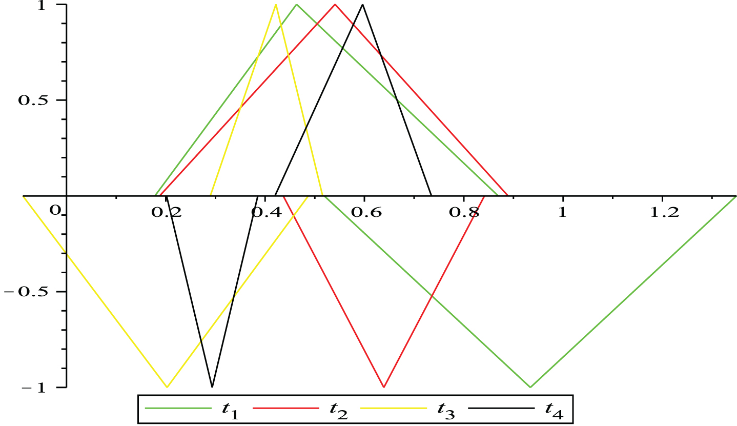
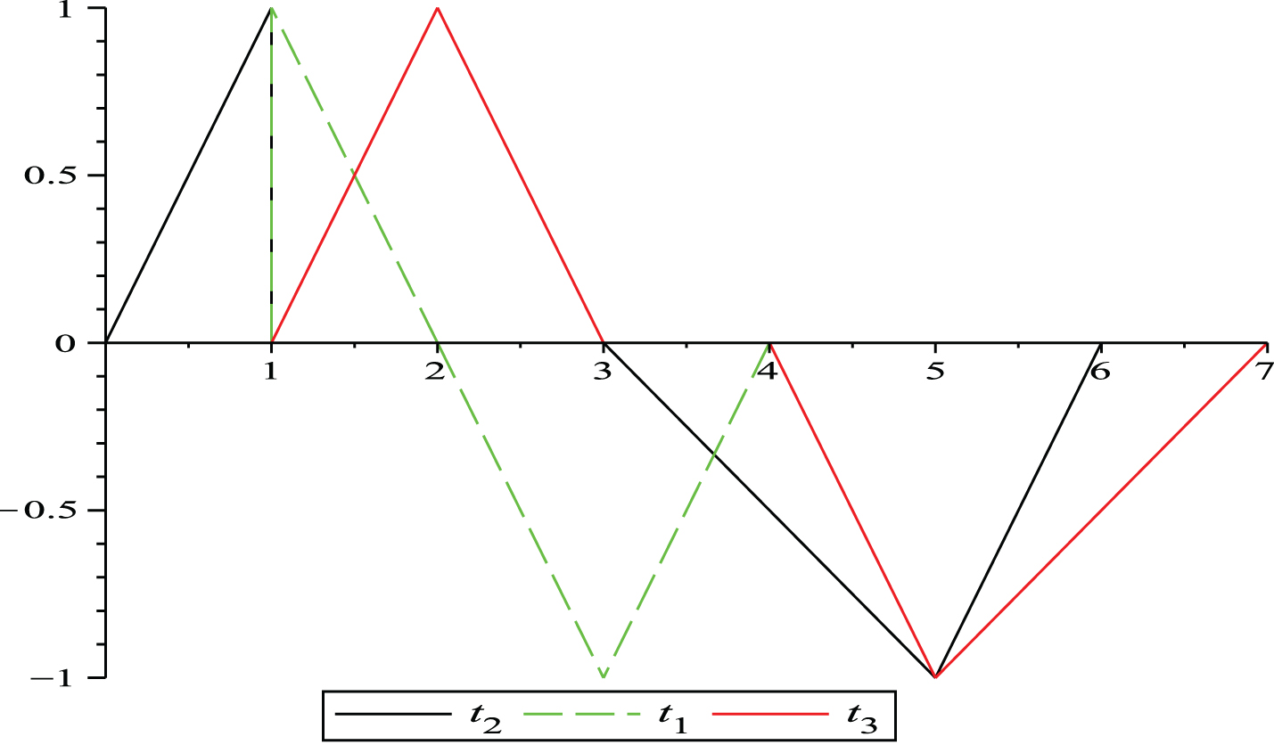
The graphical presentation of the exact solutions of both examples.

From Fig. 1, it is clear that t₁, t₂, t₃ and t₄ are bipolar fuzzy numbers.

From Fig. 2, it is clear that t₁, t₂ and t₃ are bipolar fuzzy numbers.

5.1 Comparison analysis of methods

Table 1
Comparison table of Example 5.1

Method Number of iterations Hausdroff distance

Jacobi 26 1.1000e^-05

GS 12 1.0000e^-05

GJ 11 1.0000e^-05

GGS 5 1.0000e^-05

RJ 9 1.0000e^-05

RGS 6 1.000e^-04

RGJ 6 5.0000e^-05

RGGS 4 1.0000e^-05

Method	Number of iterations	Hausdroff distance
Jacobi	26	1.1000e^-05
GS	12	1.0000e^-05
GJ	11	1.0000e^-05
GGS	5	1.0000e^-05
RJ	9	1.0000e^-05
RGS	6	1.000e^-04
RGJ	6	5.0000e^-05
RGGS	4	1.0000e^-05

Table 2

Comparison table of Example 5.2

Method	Number of iterations	Hausdroff distance
Jacobi	Diverges
GS	Diverges
GJ	11	1.0000e^-05
GGS	9	1.0000e^-05
RGJ	8	4.0000e^-05
RGGS	7	3.0000e^-05

6 Conclusions

Linear systems of equations play a vital role in many applied mathematics and applied physics. In several real problems, we have to deal with uncertain data, that is, we deal with fuzzy numbers and more generally bipolar fuzzy numbers rather than the crisp numbers. It is of much importance to develop numerical techniques that would be used to solve BFSLEs. In this document, we have introduced some iterative methods namely, generalized Jacobi (GJ), generalized Gauss-Seidel (GGS), refined Jacobi (RJ), refined Gauss-seidel (RGS), refined generalized Jacobi (RGJ) and refined generalized Gauss-seidel (RGGS) iterative methods to approximate the solution of BFSLEs. To see the performance, accuracy and efficiency of these iterative methods, we have presented some numerical examples. We have seen that our proposed methods also converge for those BFSLEs where the Jacobi and Gauss-seidel methods [6] diverge. From comparison tables, we see the validity and accuracy of proposed iterative methods. In future, we plan to extend these iterative methods to m-polar fuzzy system of linear equations.

Fig.1

The graphical presentation of exact solution of Example 5.1.

Fig.2

The graphical presentation of exact solution of Example 5.2.

Conflict of interest

The authors declare no conflict of interest.

References

Abbasbandy

, Ezzati

, Jafarian

, LU decomposition method for solving fuzzy system of linear equations, Applied Mathematics and Computation 172(1) (2006), 633–643.

Abbasbandy

, Jafarian

, Steepest descent method for system of fuzzy linear equations, Applied Mathematics and Computation 175(1) (2006), 823–833.

Abbasbandy

, Jafarian

, Ezzati

, Conjugate gradient method for fuzzy symmetric positive definite system of linear equations, Applied Mathematics and Computation 171(2) (2005), 1184–1191.

Akram

, Ali

, Allahviranloo

, Certain methods to solve bipolar fuzzy linear system of equations, Computational and Applied Mathematics (2020), 10.1007/s40314-020-01256-x.

Akram

, Arshad

, A novel trapezoidal bipolar fuzzy TOPSIS method for group decision-making, Group Decision and Negotiation 28(3) (2019), 565–584.

Akram

, Muhammad

, Ali

N.A.

, Hussain

, Iterative methods for solving a system of linear equations in a bipolar fuzzy environment, Mathematics 7(8) (2019).

Akram

, Muhammad

, Allahviranloo

, Bipolar fuzzy linear system of equations, Computational and Applied Mathematics 38(2) (2019), 69.

Akram

, Muhammad

, Hussain

, Bipolar fuzzy system of linear equations with polynomial parametric form, Journal of Intelligent and Fuzzy Systems 37 (2019), 8275–8287.

Akram

, Saleem

, Allahviranloo

, Linear system of equations in m-polar fuzzy environment, Journal of Intelligent and Fuzzy Systems 37(6) (2019), 8251–8266.

10.

Allahviranloo

, Numerical methods for fuzzy system of linear equations, Applied Mathematics and Computation 155(2) (2004), 493–502.

11.

Allahviranloo

, Successive over relaxation iterative method for fuzzy system of linear equations, Applied Mathematics and Computation 162(1) (2005), 189–196.

12.

Allahviranloo

, The Adomian decomposition method for fuzzy system of linear equations, Applied Mathematics and Computation 163(2) (2005), 553–563.

13.

Allahviranloo

, Uncertain Information and Linear Systems, Springer (2019).

14.

Allahviranloo

, Ghanbari

, On the algebraic solution of fuzzy linear systems based on interval theory, Applied mathematical Modelling 36(11) (2012), 5360–5379.

15.

Allahviranloo

, Haghi

, Ghanbari

, The nearest symmetric fuzzy solution for a symmetric fuzzy linear system, Analele Universitatii ’Ovidius’ Constanta-Seria Matematica 20(1) (2012), 151–172.

16.

Allahviranloo

, Salahshour

, Fuzzy symmetric solutions of fuzzy linear systems, Journal of Computational and Applied Mathematics 235(16) (2011), 4545–4553.

17.

Cong-Xin

, Ming

, Embedding problem of fuzzy number space: Part I, Fuzzy sets and Systems 44(1) (1991), 33–38.

18.

Dafchahi

F.N.

, A new refinement of jacobi method for solution of linear system equations, International Journal Contemporary Mathematical Sciences 3(17) (2008), 819–827.

19.

Dehghan

, Hashemi

, Iterative solution of fuzzy linear systems, Applied Mathematics and Computation 175(1) (2006), 645–674.

20.

Friedman

, Ming

, Kandel

, Fuzzy linear systems, Fuzzy sets and systems, Fuzzy Sets and Systems 96(2) (1998), 201–209.

21.

Gonfa

G.G.

, Refined iterative methods for solving system of linear equations, American Journal of Computational and Applied Mathematics 6(3) (2016), 144–147.

22.

Grzegorzewski

, Distances between intuitionistic fuzzy sets and/or interval-valued fuzzy sets based on the Hausdorff metric, Fuzzy Sets and Systems 148(2) (2004), 319–328.

23.

Saberi Najafi

, Edalatpanah,S. and Refahi Sheikhani,A., zApplication of homotopy perturbation method for fuzzy linear systems and comparison with Adomians decomposition method, Chinese Journal of Mathematics (2013).

24.

Salkuyeh

D.K.

, Generalized Jacobi and Gauss-Seidel methods for solving linear system of equations, Numerical Mathematics, A Journal of Chinese Universities (English Series) 16(2) (2007), 164–170.

25.

Vatti

, Eneyew

T.K.

, A refinement of gauss-seidel method for solving of linear system of equations, International Journal of Contemporary Mathematical Sciences 6(3) (2011), 117–121.

26.

Zhang

W.R.

, Bipolar fuzzy sets and relations: a computational framework for cognitive modeling and multiagent decision analysis, In Proceedings of IEEE Conference (1994), 305–309.

27.

Zhang

W.R.

, Bipolar fuzzy sets, IEEE International Conference on Fuzzy Systems Proceedings 1 (1998), 835–840.

Certain efficient iterative methods for bipolar fuzzy system of linear equations

Abstract

Keywords

1 Introduction

2 Preliminaries

5 Applications

5.1 Comparison analysis of methods

Table 1 Comparison table of Example 5.1 Method Number of iterations Hausdroff distance Jacobi 26 1.1000e-05 GS 12 1.0000e-05 GJ 11 1.0000e-05 GGS 5 1.0000e-05 RJ 9 1.0000e-05 RGS 6 1.000e-04 RGJ 6 5.0000e-05 RGGS 4 1.0000e-05

Conflict of interest

References

Table 1
Comparison table of Example 5.1

Method Number of iterations Hausdroff distance

Jacobi 26 1.1000e^-05

GS 12 1.0000e^-05

GJ 11 1.0000e^-05

GGS 5 1.0000e^-05

RJ 9 1.0000e^-05

RGS 6 1.000e^-04

RGJ 6 5.0000e^-05

RGGS 4 1.0000e^-05