A new adaptive variable step size natural gradient BSS algorithm

Abstract

The traditional blind source separation (BSS) algorithm is mainly used to deal with signal separation under the noiseless model, but it does not apply to data with the low signal to noise ratio (SNR). To solve the problem, an adaptive variable step size natural gradient BSS algorithm based on an improved wavelet threshold is proposed in this paper. Firstly, an improved wavelet threshold method is used to reduce the noise of the signal. Secondly, the wavelet coefficient layer with obvious periodicity is denoised using a morphological component analysis (MCA) algorithm, and the processed wavelet coefficients are recombined to obtain the ideal model. Thirdly, the recombined signal is pre-whitened, and a new separation matrix update formula of natural gradient algorithm is constructed by defining a new separation degree estimation function. Finally, the adaptive variable step size natural gradient blind source algorithm is used to separate the noise reduction signal. The results show that the algorithm can not only adaptively adjust the step size according to different signals, but also improve the convergence speed, stability and separation accuracy.

Keywords

Improved wavelet threshold function noise reduction blind source separation natural gradient adaptive variable step size

1 Introduction

Hydraulic equipment has been exposed to harsh environments such as fast speed and high temperature for a long time, and the failure rate of rolling bearings has been greatly improved. Therefore, failure analysis of rolling bearings in rotating machinery has become a top priority in the field of hydraulics. The blind source separation is a research field which developed rapidly at the end of the 20th Century, and the application of BBS in the mechanical fault diagnosis field is significant [1]. As we all know, the signals collected during the fault diagnosis process often contain a lot of noise, so the transmission channel may be interfered by the external non-stationary environment. The traditional BSS algorithms mostly separate the mixed observation signals in a stable environment. Therefore, the final result of separation is the superposition of the original signal and the noise in the actual noise model [2]. When the SNR is low, the separation performance of the BSS algorithm will be greatly reduced, which cannot achieve the expected effect. Thus, scholars at home and abroad used some noise reduction algorithms to establish filtering models and made great achievements. Protter [3] established a sparse representation model on the basis of the unitary dictionary to solve the denoising problem of Bayesian noise, and extended it to practical engineering. Guo improved the fixed basis function in wavelet transform using sparse vector and learned dictionary, and the noise reduction performance was optimized [4]. Wang [5] built a layered adaptive wavelet threshold noise reduction model to improve the shortcomings of traditional wavelet threshold method.

BSS algorithm is used to separate non-gaussian mixed signals under unknown conditions, which greatly promotes the development of signal blind processing. However, the fixed step size algorithm has some disadvantages of slow convergence speed and large error in a stable environment. In order to solve the problems, a simulated annealing algorithm was proposed, but the step size of the algorithm decreased with time, and the separation was blind [6]. Therefore, Li improved the convergence speed of BSS algorithm by fusing momentum terms, and the improved BSS algorithm could avoid segmental convergence and improve the separation performance [7]. Zhang [8] used adaptive momentum factor to optimize the variable step of the BSS algorithm, and the improved algorithm can adjust step size adaptively, which could overcome the shortcomings of blind separation. The shift-invariant wavelet denoising method was combined with the BSS algorithm to improve the performance of the algorithm in reference [9]. Since the disadvantages of traditional wavelet threshold method and the BSS algorithm cannot be improved, the denoising process is relatively slow and the requirement of fast separation cannot be satisfied.

Therefore, a new adaptive variable step size natural gradient BSS algorithm based on improved wavelet threshold is put forward in this paper. Firstly, the improved wavelet threshold method is used to process the vibration signal. Next, the wavelet coefficient

layer with obvious periodicity is denoised using the MCA, and the processed wavelet coefficients are recombined to obtain the ideal model. Then, a defined signal separation degree is brought into the separation degree estimation function, and the separation matrix update formula of the new natural gradient algorithm is constructed. Finally, the adaptive variable step size natural gradient blind source algorithm is used to separate the noise reduction signal and the steps in different stages are changed by adjusting parameters to adapt to the separation of different types signals.

2 Improved wavelet threshold function

In order to improve the noise reduction ability in the traditional wavelet transform method, the hard and soft threshold methods which could decompose and recombine the noisy signal through wavelet threshold function were proposed by Donoho [10]. However, the hard threshold wavelet denoising method has discontinuities, and the soft threshold method has constant deviation, which cannot meet the requirements of signal processing and analysis. In the reference [11], a gradual semi-soft threshold function was proposed by Zhou, which could solve the problem of the discontinuities in the hard threshold method, but the signal processed by the method still had a large deviation from the original signal. Subsequently, an improved exponential threshold function denoising method was proposed in the reference [12], which could solve the problems of the hard threshold method and soft threshold method to some extent. Nevertheless, due to the lack of adjustment factors, the adaptability to different noises is poor and the noise reduction effect is not good.

An adaptive wavelet threshold denoising method is proposed in this paper to improve the existing problems of wavelet threshold, which can not only effectively overcome the shortcomings of the problems in the existing wavelet thresholds, but also improve the adaptability.

2.1 Improved sparse wavelet threshold function

The threshold function expression can be described as follows: $\bar{w_{j, k}} = {\begin{matrix} λ \times w_{j, k} + (1 - λ) \times sgn (w_{j, k}) \times (| w_{j, k} | - \frac{2 \times η}{1 + {log}_{δ}^{(δ + a \times (| w_{j, k} | - η)^{n})}}) & | w_{j, k} | ⩾ η \\ 0 & | w_{j, k} | < η \end{matrix}$ (1)

Where $\bar{w_{j, k}}$ is the adaptive wavelet coefficient, λ = 1 - e ^{-β×(|w_j,k|-η)²}. When β > 0, δ > 1 and a > 0, then λ ⊂ [0, 1]. In addition, η is the wavelet threshold, $η = ɛ \times \sqrt{2 ln (N)}$ , N is the signal length, and usually n→ + ∞. ɛ is the root mean square error of the noise [13], and ɛ = median (|x|)/0.6745.

2.2 Theoretical analysis of the improved threshold function

(1) Proof process of the continuity $y = lim_{w_{j, k \to} η^{+}} {\bar{w}}_{j, k}$ $= lim_{w_{j, k} \to η^{+}} (λ \times w_{j, k} + (1 - λ) \times (| w_{j, k} | - η))$ $= lim_{w_{j, k} \to η^{+}} (| w_{j, k} | - η + λ \times η)$ $∵ y_{1} = lim_{w_{j, k} \to η^{+}} λ = lim_{w_{j, k} \to η^{+}} (1 - e^{- β \times (| w_{j, k} | - η)^{2}})$ $= 1 - e^{0} = 0$ $∴ y = lim_{w_{j, k} \to η^{+}} (| w_{j, k} | - η + λ \times η) = 0$

The following conclusion can be proved by the same method: $y^{'} = lim_{w_{j, k} \to η^{-}} \bar{w_{j, k}} = 0$

It can be seen that the new threshold function is not interrupted at points ±η,which can solve the discontinuity problem in the hard threshold method.

(2) Proof process of the deviation $x = lim_{w_{j, k} \to + \infty} (\bar{w_{j, k}} - w_{j, k})$ $= lim_{w_{j, k} \to + \infty} (λ \times w_{j, k} + (1 - λ) \times (w_{j, k} - η) - w_{j, k})$ $= lim_{w_{j, k} \to + \infty} (η \times (λ - 1))$ $\begin{matrix} ∵ x_{1} = lim_{w_{j, k} \to + \infty} λ = lim_{w_{j, k} \to + \infty} (1 - e^{- β \times (| w_{j, k} | - η)^{2}}) \\ = 1 - e^{lim_{w_{j, k} \to + \infty} (- β \times (| w_{j, k} | - η)^{2})} = 1 - e^{- \infty} = 1 \end{matrix}$ $∴ x = lim_{w_{j, k} \to + \infty} (η \times (λ - 1)) = 0$

The following conclusion can be proved by the same method: $x^{'} = lim_{w_{j, k} \to - \infty} (\bar{w_{j, k}} - w_{j, k}) = 0$

According to the deviation analysis of the new threshold function, when w_j,k→ ∞, the new wavelet threshold function $\bar{w_{j, k}}$ approaches to w_j,k, which greatly improves the problem of constant deviation in the soft threshold wavelet method.

(3) Analysis of threshold adjustment factors

a) When β = 0 and η→ + ∞, then $λ = 1 - e^{- β \times (| w_{j, k} | - η)^{2}} = 1 - e^{0} = 0 .$

b) $z = lim_{η \to + \infty} {\bar{w}}_{j, k}$ , and λ = 0 is brought into z. When w_j,k ⩾ η, then z = sgn (w_j,k) × (|w_j,k| - η), otherwise, z = 0.

c) When β→ + ∞ and λ = 1 - e ^{-β×(|w_j,k|-η)²} = 1 - e ^-∞ = 1, then λ = 1 is brought into z. When w_j,k ⩾ η, then z = w_j,k, otherwise, z = 0.

It can be seen that the new threshold function can be transformed into the hard threshold function or the soft threshold function smoothly by adjusting parameter β, which shows that it has high flexibility and strong adaptability. And the new threshold function can make up for the defects of the threshold function mentioned in reference [11] and [12]. Noise reduction contrast diagram of different threshold functions is shown in Fig. 1, and the adjustment effect of β value on the new threshold function is shown in Fig. 2.

Fig. 1

The noise reduction curves of different threshold functions.

Fig. 2

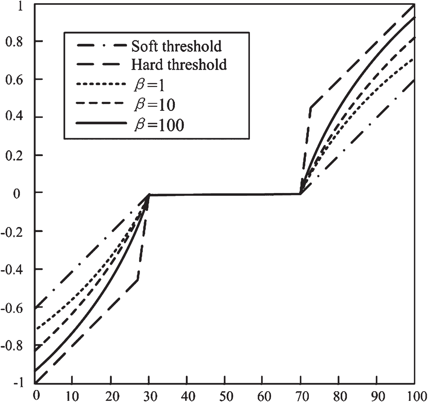
The adjustment effect of β value on the new threshold function.

It can be seen from Fig. 1 that the hard threshold function noise reduction signal is close to the original signal with a value of one, but there is a problem of discontinuity. Although the problem of discontinuous points is solved by the soft threshold, the difference between the noise reduction signal and the original signal is about 0.4, which indicates that the soft threshold function noise reduction signal is different from the original signal, and there is a constant deviation. The signal processed by the threshold function in reference [11] still has a large deviation from the original signal, and the threshold adjustment method in reference [12] is not flexible enough to adapt to different noise environments. As can be seen from Fig. 2, when the value increases from 1 to 100, the new threshold function gradually realizes the conversion from the soft threshold to the hard threshold, and basically converges to the original signal. Therefore, the new threshold function proposed in this paper can not only reduce the noise of the collected signal and retain the effective signal characteristics to the greatest extent, but also adjust parameters to adapt to different condition.

2.3 Morphological component analysis (MCA)

Signals in practical engineering usually can be converted to sparse form or have sparse form after processing, so the decomposed wavelet coefficients are denoised in this paper. Because the independent component analysis method has a very low probability that the two source signals are useful signals under independent assumptions, the method cannot always achieve good results. Therefore, the mixed signal is composed of multiple signals with sparse characteristics, and the MCA proposed by Starck is used for the separation of mixed signals [14]. The specific principle is as follows:

Suppose that the source signal l is a linear combination of R different morphological component signals l_r, and it can be expressed as $l = \sum_{r = 1}^{R} l_{r}$ . Where, each l_r component can be represented by its own over-complete dictionary Φ_r, and it can be written as l_r = Φ_rd_r, d_r is the decomposition coefficient. Therefore, the sparsest representation of l is converted into the optimal solution of Equation (2). $min_{d_{1}, \dots, dR} \sum_{r = 1}^{R} | d_{r} |_{1} l = \sum_{r = 1}^{R} Φ_{r} d_{r}$ (2)

Equation (2) can be approximately expressed as follows: $min_{d_{1}, \dots, dR} \sum_{r = 1}^{R} | d_{r} |_{1} + η | l - \sum_{r = 1}^{R} Φ_{r} d_{r} |_{2}^{2}$ (3)

Where, η is a given threshold value, and the sparse representation d_r of signal l_r is written as: $l_{r} = Φ_{r}^{*} l_{r} Φ_{r}^{*} = Φ_{r}^{T} (Φ_{r} Φ_{r}^{T})^{- 1}$ (4)

Therefore, the solution of the decomposition coefficient d_r can be transformed into the solution of the signal l components {l₁, ⋯ , l_R }. ${l_{1}, \dots, l_{R}} = arg min_{l_{1}, \dots, lR} \sum_{r = 1}^{R} | Φ_{n}^{*} s_{k} |_{1} + η_{n} | l - \sum_{r = 1}^{R} s_{r} |_{2}^{2}$ (5)

In order to verify the effectiveness of the MCA sparse representation for wavelet noise reduction algorithm, simulation analysis on impact signal is carried out by analogue fault signals [15]. The observation signal f_(t) and impact signal ρ_(t) are denoted as: ${\begin{matrix} f_{(t)} = ρ_{(t)} + ν_{(t)} \begin{matrix} \begin{matrix} \begin{matrix} \begin{matrix} \end{matrix} \end{matrix} \end{matrix} \end{matrix} \\ ρ_{(t)} = \sum_{k} e^{\frac{- χ_{0}}{\sqrt{1 - χ_{0}^{2}}} [2 π f_{0} (t - kT - τ_{0})]} cos (2 π f_{0} (t - kT - τ_{0})) \end{matrix}$ (6)

Where, the frequency f₀ = 10Hz, damping ratio χ₀ = 0.01, delay constant τ₀ = 1, impact period T = 2s, v_(t) is noise interference, and the simulation steps are as follows:

Firstly, the observed signal f_(t) is denoised according to Equation (1), and a series of wavelet coefficients are obtained. Secondly, the wavelet coefficients with strong periodicity are selected and denoised using the MCA. Finally, the denoised wavelet coefficients are recombined to obtain the effective signal. Figure 3 shows results of the simulation signal direct reconstruction and reconstruction after MCA noise reduction. The results show that the direct denoising recombination signal noise is more thoroughly filtered comparing with the MCA denoising recombination signal, but the impact characteristics are not effectively described.

Fig. 3

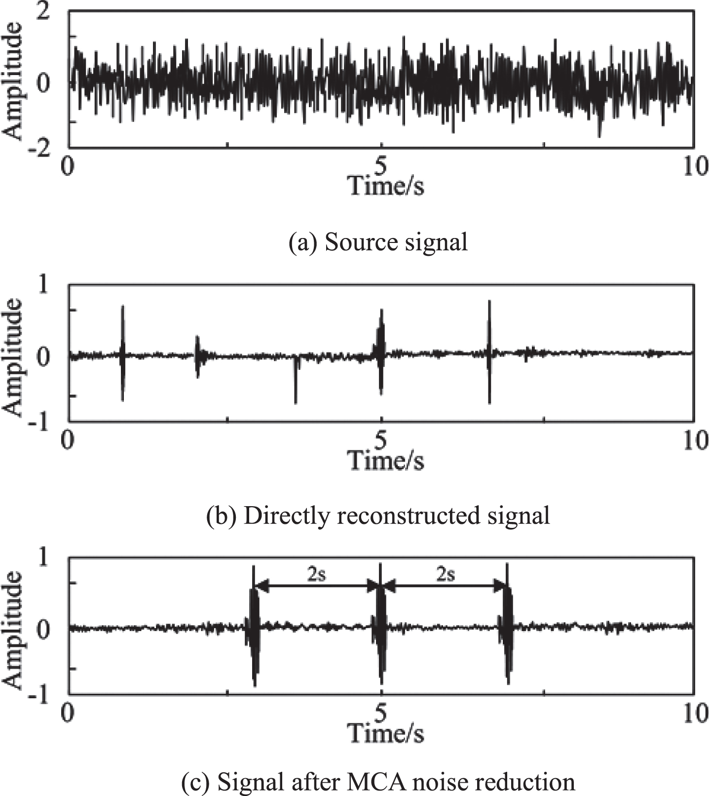
Simulation signal reconstruction and MCA noise reduction reconstruction results.

3 Adaptive variable step size algorithm

The BSS model with noise can be described as: $h_{(t)} = A \times g_{(t)} + w_{(t)}$ (7)

Where, h_(t) = [h_1(t), ⋯ , h_m(t)] is m noise signals observed. g_(t) = [g_1(t), ⋯ , g_n(t)] is the n source signals which are generally assumed to be statistically independent from each other. A is a m × n -dimensional mixed matrix with full column rank. w_(t) is the collected noise signal, and m > n. In the noiseless model (in the case where both A and g_(t) are unknown), the BSS algorithm is used to find a de-mixing matrix B, and B ≈ A ^-1, i.e. A × B ≈ I.

3.1 Description of natural gradient algorithm

The key to blind separation is to find the optimal de-mixing matrix B, so that each signal component G_(i) is independent. Kullback-Leibler divergence I_(B) is usually used as the independence measure and minimized [16]. The formula is expressed as follows: $I_{(B)} = \int p (G; B) lg \frac{p (G; B)}{\prod_{i = 1}^{n} p_{i} (G_{i}; B)} dG$ (8)

Where, p (G) is the joint probability density function of G. p_i (G_i) is the edge probability density function of G. Only if P (G ; B) and p_i (G_i ; B) have the same distribution, the divergence I_(B) is zero, and it does not change with the nonlinear transformation of the variable G_i. In this case, the separation effect is ideal. The stochastic gradient algorithm of the separation matrix B is expressed as: $B_{(t + 1)} = B_{(t)} + M_{(t)} \times [B_{(t)}^{- 1} - f_{(G)} \times G^{T}] \times B_{(t)}$ (9)

However, the stochastic gradient algorithm has some defects, such as slow convergence speed, great influence by the mixed matrix A, and the need to solve the inverse matrix in the iterative process. Therefore, the natural gradient algorithm has been proposed and the formula is as follows: $B_{(t + 1)} = B_{(t)} + M_{(t)} \times [I - f_{(G)} \times G^{T}] \times B_{(t)}$ (10)

Where, M_(t) depends on the learning rate of t, and $f_{(\begin{matrix} G \end{matrix})}$ is the evaluation function. f (G) = (f₁ (G₁) , ⋯ , f_n (G_n)) is a column vector, and its definition is as follow: $f_{i} (G_{i}) = - \frac{p_{i}^{'} (G_{i})}{p_{i} (G_{i})}$ (11)

If the source signal is non-gaussian, f_i (G_i) is a nonlinear function.

3.2 Adaptive variable step size algorithm

The fixed step size is usually used in the traditional natural gradient algorithm, but it has some defects, such as the low convergence speed and large steady-state error. Therefore, the simulated annealing variable step algorithm has been proposed by some scholars to solve the defects [17]. However, the step size of this algorithm decreases as time goes on, and the separation is blind, which shows the algorithm cannot achieve the desired effect. In order to solve the problems, an adaptive variable step size natural gradient BSS algorithm based on improved wavelet threshold is put forward in this paper. The defined signal separation degree is introduced into the separation degree estimation function, and a new separation matrix update formula of natural gradient algorithm is constructed. The separation process is divided into several stages, and each stage adopts different steps, which can improve the convergence speed and stability.

According to the separation matrix update formula of the traditional natural gradient algorithm, if the algorithm converges, then the de-mixing matrix B (t) ≠0 and the step size M (t) ≠0. The following formula can be obtained: $lim_{k \to \infty} (I - f_{(G (t))} \times G_{(t)}^{T}) = 0$ (12)

Therefore, D (t) is the Frobe-nius norm square of the resolution, and it is used as the separation degree value, which can be described as follows: $D (t) = | I - f_{(G (t))} \times G_{(t)}^{T} |_{F}^{2}$ (13)

The separation degree estimation function Q (t) is defined according to the crosstalk error formula, and D (t) is brought into Q (t). The new separation degree estimation function is described as: $\begin{matrix} Q (t) = \sum_{i = 1}^{n} ((\sum_{j = 1}^{n} \frac{| D_{t} (i, j) |}{max | D_{t} (i, \cdot) |} - 1) \\ + (\sum_{j = 1}^{n} \frac{| D_{t} (i, j) |}{max | D_{t} (\cdot, j) |} - 1)) \end{matrix}$ (14)

In order to change step size adaptively, the Frobe-nius norm square of the instantaneous error signal is used to control the error variation. The error function F (t) is defined as: $F (t) = | B \times B^{T} - I |_{F}^{2}$ (15)

It can be seen from the Equation (15) that F (t) is always more than zero to prevent the large fluctuation of step size in the separation process. According to the experimental requirements, the upper and lower limit of step size are set as M_max = 0.05 and M_min = 5 ×10^-6, respectively. When the step size is between M_max and M_min, the defined error is used to update the step size. The adaptive variable step size function based on Q (t) and F (t) is as follows:

(1) When M_(t) < M_min, M_t+1 = M_min;

(2) When M_(t) > M_max, M_t+1 = M_max;

(3) When M_(t) ∈ [M_min, M_max], $M (t + 1) = {\begin{matrix} ϕ (t) \times M (t) & Δ F (t + 1) < Δ F (t) \\ γ \times M (t) + (1 - γ) \times (\frac{1}{1 + exp (- ϖ \cdot Q (t))} - \frac{1}{2}) \times F (t) & Δ F (t + 1) ⩾ Δ F (t) \end{matrix}$ (16)

Where, γ is the adjustment parameter, and the error variation ΔF (t) = F (t) - F (t - 1) is used to judge the step size. If ΔF (t) increases, it means that the step size is too large, which will cause turbulence. Therefore, a parameter ϕ (t) should be introduced to control ΔF (t), and ϕ (t) is close to but not more than one. ϕ (t) is defined as: $ϕ (t) = \frac{1 + exp (- ϖ \times Q (t))}{2}$ (17)

Where, ϖ is used to adjust the parameter ϕ (t), which can be obtained through experiments. According to the needs of this article, γ = 0.975, ϖ = 1 ×10^-3 are set. Therefore, the improved separation matrix of the new natural gradient algorithm is described as: $B (t + 1) = B (t) + M (t + 1) \times [I - f_{(G)} \times G^{T}] \times B_{(t)}$ (18)

4 The separation process of adaptive blind source algorithm

The traditional BSS algorithm is mainly used to deal with signal separation under the noiseless model. Therefore, an adaptive variable step size natural gradient BSS algorithm based on improved wavelet threshold is proposed. The signal denoising separation process diagram is shown in Fig. 4.

Fig. 4

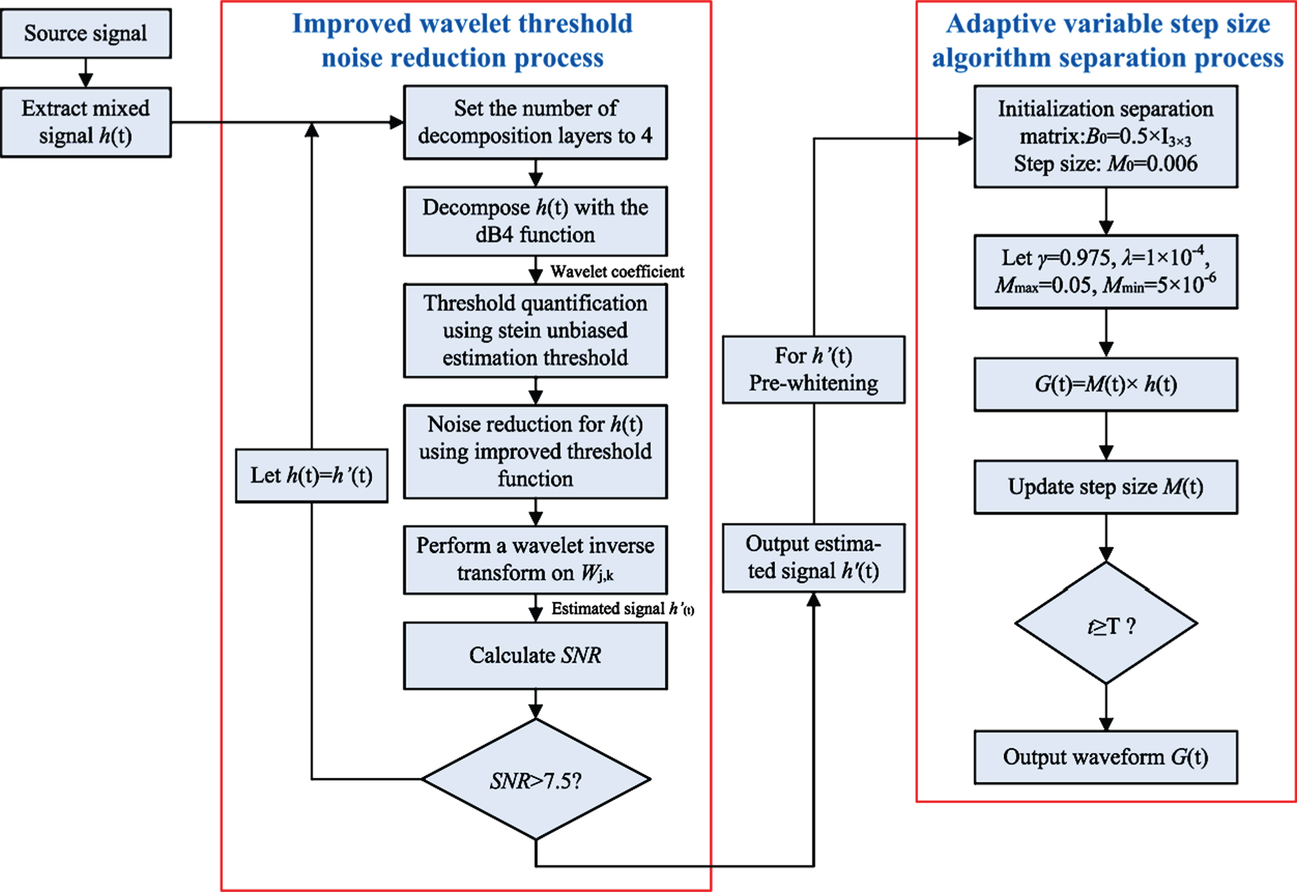
Signal denoising separation process diagram.

The steps are as follows:

The mixed signals are extracted from different types of signals.

The improved wavelet threshold denoising method is used to reduce the noise of mixed signals.

The separation matrix is initialized as B₀ = 0.5 × I_3×3, the initial step size and parameters are set as: m₀ = 0.006. γ = 0.975, ϖ = 1 ×10^-4, M_max = 0.05, M_min = 5 ×10^-6.

Separation calculation is performed according to the formula G_(t) = M_(t) × h_(t).

Step size is updated as M_(t).

When t ⩾ T, then return to step (5) to cycle. otherwise, the separated waveforms are drawn according to the output G_(t), and comparison of various crosstalk errors are obtained.

5 Simulation analysis

5.1 Denoising effect analysis of improved wavelet threshold function

In order to verify the noise reduction effect of the wavelet threshold function proposed in this paper, the hard threshold function, the soft threshold function, the semi-soft threshold function, the function in reference [12] and the new wavelet threshold function method are used to reduce the noise of a sinusoidal signal mixed with noise respectively.

The signal in MATLAB is adopted, and it is composed of sinusoidal signal and white noise signal. The function can be described as Equation (19), and its signal parameters are shown in Table 1. $s (t) = sin (0.03 t) + b_{1} (t)$ (19)

Table 1

Signal parameters

Function	Number of points	Byte	Type
Noissin	1*1000	8000	Double

The wavelet noise reduction programs are written in MATLAB. Firstly, dB wavelet is used to decompose the signal, and the number of decomposition layers is 4. Then, the new threshold function is used to calculate the threshold value of the wavelet coefficient. Next, the wavelet coefficients with strong periodicity are selected and the MCA algorithm is used to deal with the noise reduction. Finally, the wavelet coefficient is reconstructed. The noise reduction curves with different wavelet threshold methods are shown in Fig. 5.

Fig. 5

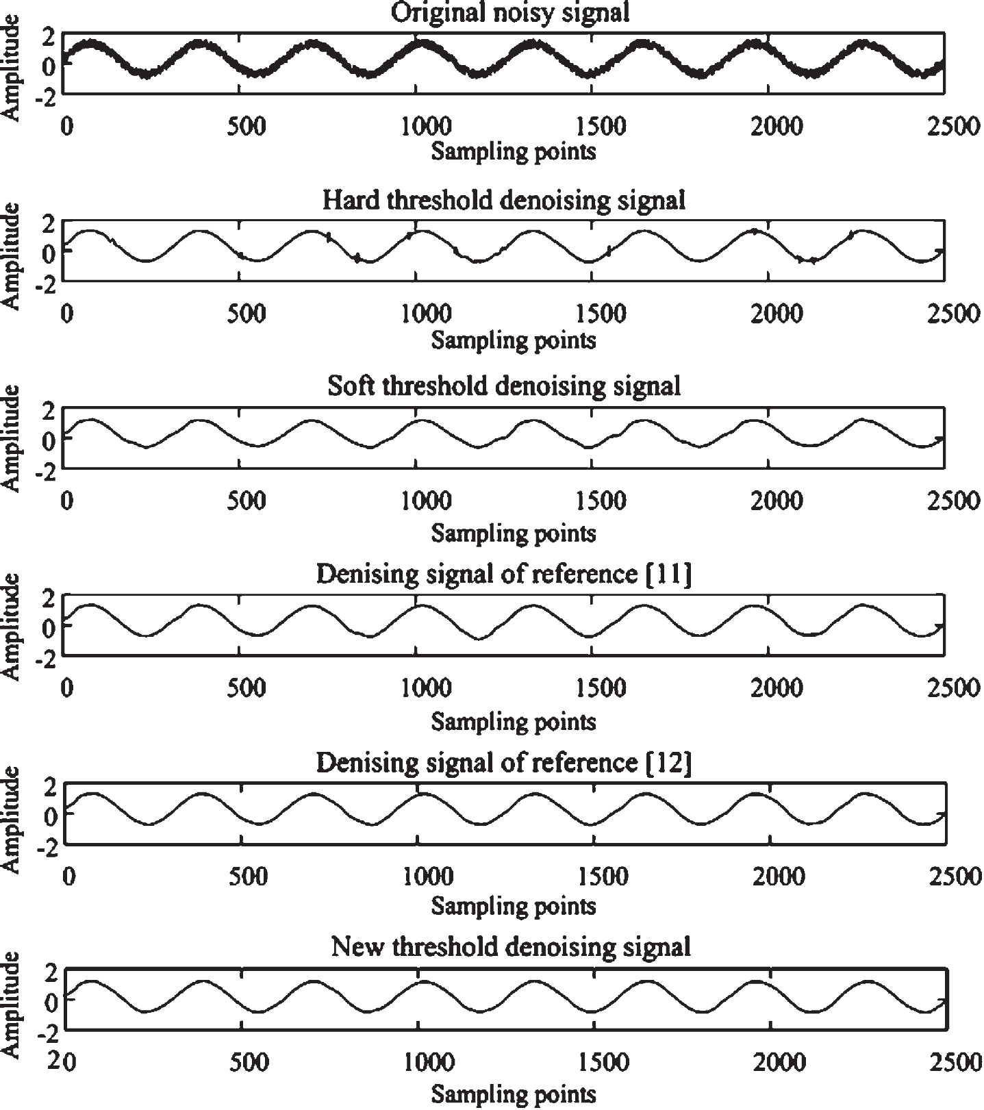
The noise reduction curves with different wavelet threshold methods.

It could be seen from Fig. 5 that the collected original signal contained a lot of noise, and there were still burrs and discontinuities in the noise reduction curve of the hard threshold method. Although there was no discontinuity in the noise reduction curve of the soft threshold method, the difference between the noise-reduced signal and the original signal was large, and this phenomenon showed that some effective information had lost after being processed by the soft threshold function. Due to the lack of adjustment parameters in semi-soft threshold noise reduction and the threshold noise reduction method in reference [12], the peak and bottom values of the noise reduction signal were still significantly different from the original signal, and the traditional threshold problem had not been solved well. The new threshold noise reduction method could not only solve the problem of discontinuity, but also improve the issue of constant deviation. And the noise-reduced signal basically converged to the original signal, which indicated the noise reduction effect had improved significantly.

In order to further verify the superiority of the noise reduction effect of the new threshold function, the experiment was carried out using the 6205-2RS deep groove bearing vibration data from the Data Center of Case Western Reserve University. In addition, the fast Fourier transform (FFT) was used to analyze the bearing vibration signal in frequency domain. Figure 6 showed bearing fault signal FFT spectrum of different threshold function for noise reduction.

Fig. 6

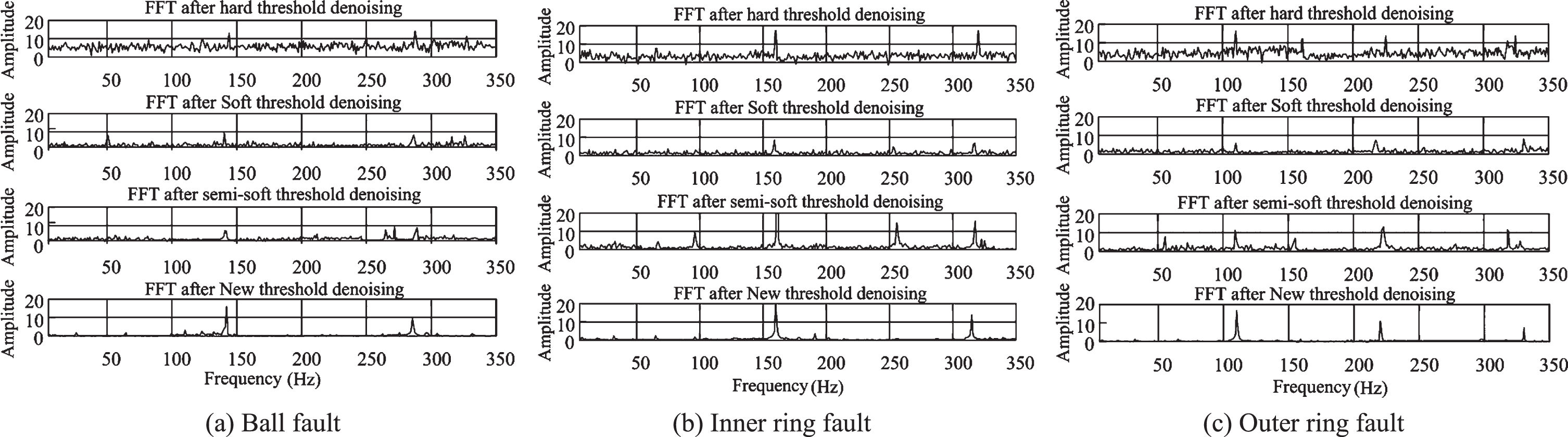
Bearing fault signal FFT spectrum of different threshold function for noise reduction.

It can be seen from Fig. 6 that the noise filtering of the hard threshold noise reduction was not thorough and the energy was not concentrated, so the bearing fault type could not be accurately determined. The soft threshold could filter the noise better, but its amplitude was lower than the original signal, so it could filter some effective signals in the noise reduction process. Although semi-soft threshold noise reduction method improved the shortcomings of soft and hard threshold noise reduction method, the crests and troughs values appeared irregularly, and the judgment reliability could not be guaranteed. The new threshold function proposed in this paper was used for noise reduction of bearing fault signal, and the results showed that the peak value appeared near 140 Hz, 160 Hz, 110 Hz and their multiples in Fig. 6(a)–(c) respectively, which corresponded to the theoretical calculation value. Therefore, the accuracy of fault diagnosis was increased after the noise reduction of the new threshold in this paper.

Signal to noise ratio (SNR) and root mean square error (RMSE) of the five threshold functions were calculated by MATLAB. Table 2 showed the noise reduction effect evaluation of different wavelet threshold algorithms.

Table 2

Noise reduction effect evaluation of different wavelet threshold algorithms

Fault type	Evaluation index	Hard threshold	Soft threshold	Reference [11]	Reference [12]	New threshold
Ball failure	SNR(dB)	2.8250	3.0129	7.3354	8.8624	9.5327
	RMSE(×10^-4)	0.6832	0.6641	0.6216	0.6153	0.5804
Inner ring failure	SNR(dB)	2.2431	2.8156	6.4257	7.2315	9.3251
	RMSE(×10^-4)	0.7351	0.7112	0.6841	0.6766	0.6105
Outer ring failure	SNR(dB)	2.7632	3.5624	6.1388	8.4513	10.0726
	RMSE(×10^-4)	0.5271	0.4868	0.4032	0.3808	0.3016

From Table 2, it could be clearly seen that the SNR of the new threshold algorithm in this paper was much higher than that of other threshold functions for different fault types. RMSE was lower than that of other threshold functions, indicating that the algorithm in this paper could not only improve the SNR and stability, but also greatly increase the accuracy of bearing fault diagnosis.

5.2 Analysis of adaptive variable step size separation algorithm based on improved wavelet threshold

In this experiment, the noise signals were added to five types of easy-to-observe signals, and the mixed signals were chosen as source signals. The signal functions can be expressed as follows:

(1) Symbol signal: m_1(t) = sign (cos(2 × π × 150t));

(2) High frequency sinusoidal signal:

m_2(t) = sin(2 × π × 780t);

(3) Phase modulation signal:

m_3(t) = sin(2 × π × 300t + 60 × cos(2 × π × 60t));

(4) Low frequency sinusoidal signal: m_4(t) = sin(2 × π × 80t);

(5) Random noise uniformly distributed in [-1,1].

The source signal waveforms were shown in Fig. 7.

Fig. 7

Five types source signal waveforms.

The five signals were tested according to the separation process in part 4. Figures 8 and 9 are the mixed signal diagrams and the mixed signal diagrams processed by the improved wavelet threshold denoising method respectively. It could be seen that the signal burrs processed by the improved wavelet threshold denoising method reduced significantly through comparative analysis.

Fig. 8

Mixed signal diagram.

Fig. 9

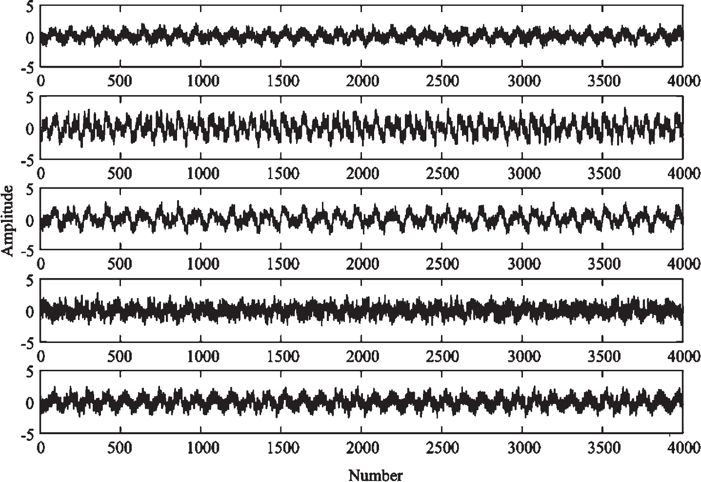
Mixed signal diagrams processed by the improved wavelet threshold denoising method.

The mixed signals were denoised by the new threshold wavelet function, and the fixed step method, simulated annealing algorithm, symbolic natural gradient algorithm and the adaptive variable step size algorithm were adopted to separate the processed signal respectively. The output waveform was extracted and the crosstalk error of different separation algorithms was calculated. The separation results of different BSS algorithms were shown in Fig. 10.

Fig. 10

Separation results of different BSS algorithms.

As seen from Fig. 10, the output waveform processed by the fixed step algorithm fluctuated greatly and had many bumps, indicating that the modulated signal had many glitches and was not standardized. Although the output waveform of the signal separated by the simulated annealing algorithm fluctuated small, there was still some noise in the separated signal, and the separation effect was irrational. The symbolic natural gradient algorithm has a better separation effect on low-frequency and high-frequency sinusoidal signals, but the output results of the remaining three algorithms was still affected by interference and the effective signal separation was not complete. The waveform separated by the method proposed in this paper was more standardized and smoother, which showed that the method could not only separate the effective signal better, but also maintain the effective characteristics of the signal.

In order to further verify the effectiveness of the adaptive variable step size algorithm, the crosstalk error was simulated and the results were shown in Fig. 11. Crosstalk error comparison diagram with different step length of the fixed step size algorithm was shown in Fig. 11 (a), and crosstalk error comparison diagram of the five algorithms was shown in Fig. 11 (b).

Fig. 11

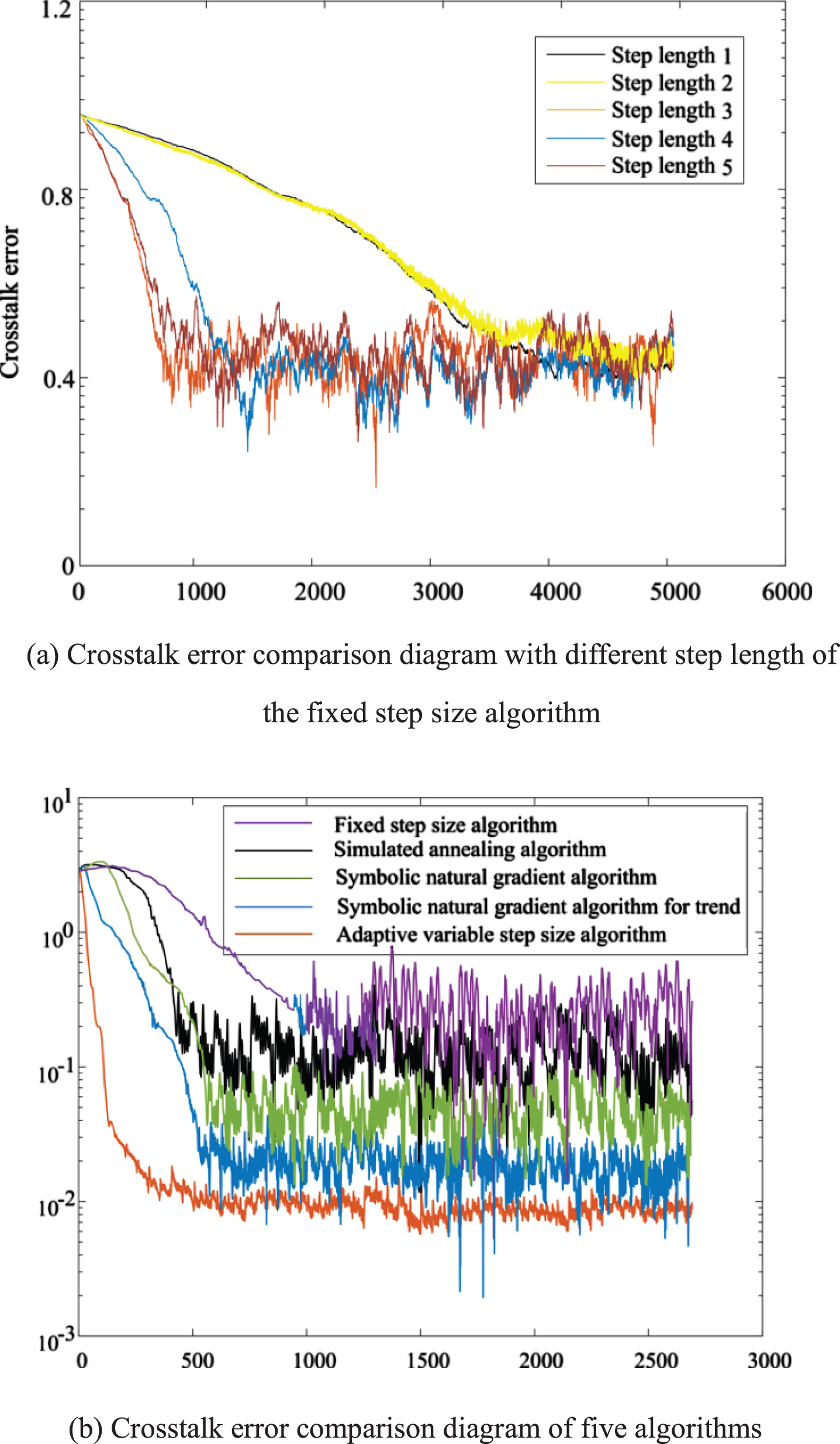
Crosstalk error comparison diagram.

It could be seen from Fig. 11(a) that the longer the step length, the faster the convergence speed, and the curve converged at about 800. Although the converged value was about 0.4, but it fluctuated greatly. The result showed that the convergence speed of the fixed step algorithm was slow and the error was large, which could not achieve the expected separation effect.

From Fig. 11 (b), it could be seen that the fixed step size algorithm fluctuated greatly and tended to be stable at 1000 sampling points, and the converged value was around 0.4. The simulated annealing algorithm, the symbol separation algorithm and the symbol separation algorithm with dynamic vectors converged at 700 points, and the steady-state error was around 0.03. However, the adaptive variable step size algorithm converged at about 300, the converged value was between 0.009 and 0.012, and the fluctuation range was small. Comparison diagram showed that the adaptive variable step size algorithm could not only adjust the step size adaptively according to different working conditions, but also have fast convergence speed and almost no error, which could effectively separate vibration signals.

6 Conclusion

Due to the influence of external interference on the transmission channel, the mixing matrix of the traditional BSS algorithm is random and dynamic time-varying. However, the traditional fixed step algorithm cannot accurately separate the effective signals in the noisy model. Therefore, a new wavelet threshold noise reduction and adaptive blind source gradient algorithm are proposed in this paper, which effectively reduce the influence of noise interference on the separation model, and a solid theoretical foundation is laid for the development of the fault diagnosis. The innovations are as follows:

In order to improve the defects of the hard threshold, the soft threshold and the threshold functions mentioned in reference [11] and [12], a wavelet threshold function based on morphological component analysis is proposed, which can improve SNR and lay a foundation for signal separation.

A separation degree estimation function and an error function are proposed. The defined signal separation degree is introduced into the separation degree estimation function, and a new separation matrix update formula of natural gradient algorithm is constructed. The step size can be controlled by ϕ (t), and the adjustment parameter ϕ (t) can be changed according to the error value.

(3) The shortcomings of traditional BSS algorithm such as noise interference and slow convergence speed are solved by the proposed method, and the effectiveness of the separation signal is guaranteed. However, the algorithm proposed in this paper is mainly used to separate the single fault signal characteristics, and the separation of complex multi-feature signals requires further study.

References

Huang

M.T.

, Lee

C.H.

and Lin

C.M.

, Blind source separation with adaptive learning rates for image encryption, Journal of Intelligent & Fuzzy Systems 30(1) (2016), 451–460.

Vazquez

R.R.

, Velez-Perez

, Ranta

, Dorr

V.L.

, Maquin

and Maillard

, Blind source separation, wavelet denoising and discriminant analysis for EEG artefacts and noise cancelling, Biomedical Signal Processing and Control 7(4) (2012), 389–400.

Protter

, Yavneh

and Elad

, Closed-form MMSE estimation for signal denoising under sparse representation modeling over a unitary dictionary, IEEE Transactions on Signal Processing 58(7) (2010), 3471–3484.

Guo

, Gao

H.L.

, Li

, Huang

H.F.

and Zhang

X.C.

, Machinery vibration signal denoising based on learned dictionary and sparse representation, 11th International Conference on Damage Assessment of Structures (Damas 2015) 628 (2015).

Wang

, Li

T.Y.

, Gao

X.J.

and Gao

H.H.

, Bearing fault signal denoising method of hierarchical adaptive wavelet threshold function, Journal of Vibration Engineering 32(03) (2019), 548–556.

Bouleimen

and Lecocq

, A new efficient simulated annealing algorithm for the resource-constrained project scheduling problem and its multiple mode version, European Journal of Operational Research 149(2) (2003), 268–281.

C.T.

, Jiang

Y.Z.

, Liu

F.J.

and Zhang

S.X.

, Step-size adaptive blind source separation algorithm with adding momentum term, Journal of Naval University of Engineering 31(03) (2019), 107–112.

Zhang

T.Q.

, Ma

B.Z.

, Qiang

X.Z.

and Quan

S.R.

, Variable-step blind source separation method with adaptive momentum factor, Journal of Communications 38(03) (2017), 16–24.

J.M.

, Zhu

X.L.

and Zhang

X.D.

, Adaptive blind separation with anunknown number of sources, Neural Computation 16(8) (2004), 1641–1660.

10.

Donoho

D.L.

and Johnstone

I.M.

, Ideal spatial adaptation by wavelet shrinkage, Biometrika 81(3) (1994), 425–455.

11.

Zhou

X.F.

, Zhu

W.W.

and Guo

Q.G.

, The denoising of ultrasonic signal based on asymptotic semi-soft thresholding function, Journal of Detection & Control 33(02) (2011), 35–39.

12.

Huang

Y.C.

and Hou

D.W.

, Fingerprint de-noising based on improved wavelet threshold function, Computer Engineering and Applications 50(06) (2014), 179–181.

13.

Hussein

, Shaban

K.B.

and El-Hag

A.H.

, Energy conservation-basedthresholding for effective wavelet denoising of partial dischargesignals, Iet Science Measurement & Technology 10(7) (2016), 813–822.

14.

Y.G.

, Zhao

G.L.

, Ma

C.Y.

and Hou

S.F.

, Denoising method based ondual-tree complex wavelet transform and MCAand its application in gear fault diagnosis, Journal ofAerospace Power 31(01) (2016), 219–226.

15.

Zhong

Y.P.

and Chen

, Application of K-SVD wavelet denoising to gear fault diagnosis, Noise and Vibration Control 36(03) (2016), 179–183.

16.

Ballesteros

J.A.

, Fernandez

M.D.

and Ballesteros

M.J.

, Application of signal preprocessing and blind source separation to sound power mesurement of machines, Noise Control Engineering Journal 64(06) (2016), 753–765.

17.

Park

, Amari

S.I.

and Fukumizu

, Adaptive natural gradient learning algorithms for various stochastic models, Neural Networks 13(7) (2000), 755–764.