Polynomial approximation to manifold learning

Abstract

Manifold learning plays an important role in nonlinear dimensionality reduction. But many manifold learning algorithms cannot offer an explicit expression for dealing with the problem of out-of-sample (or new data). In recent, many improved algorithms introduce a fixed function to the object function of manifold learning for learning this expression. In manifold learning, the relationship between the high-dimensional data and its low-dimensional representation is a local homeomorphic mapping. Therefore, these improved algorithms actually change or damage the intrinsic structure of manifold learning, as well as not manifold learning. In this paper, a novel manifold learning based on polynomial approximation (PAML) is proposed, which learns the polynomial approximation of manifold learning by using the dimensionality reduction results of manifold learning and the original high-dimensional data. In particular, we establish a polynomial representation of high-dimensional data with Kronecker product, and learns an optimal transformation matrix with this polynomial representation. This matrix gives an explicit and optimal nonlinear mapping between the high-dimensional data and its low-dimensional representation, and can be directly used for solving the problem of new data. Compare with using the fixed linear or nonlinear relationship instead of the manifold relationship, our proposed method actually learns the polynomial optimal approximation of manifold learning, without changing the object function of manifold learning (i.e., keeping the intrinsic structure of manifold learning). We implement experiments over eight data sets with the advanced algorithms published in recent years to demonstrate the benefits of our algorithm.

Keywords

Out-of-sample new data polynomial dimensionality reduction manifold learning

1 Introduction

With the rapid development of artificial intelligence, large-scale data has penetrated into various fields of real life, such as pattern recognition, text analysis, image processing, speech recognition, gene expression, etc. The huge amount of data provides researchers with rich and various information, but it also increases the difficulties of data analysis and processing. High-dimensional data usually contains lots of redundant information, which increase the complexity and computation cost of the data analysis, even cause dimensional disaster or interfere with data analysis. How to obtain effective information from high-dimensional data is a hot topic in current research of data science. The common method to solve these problems is the data dimensionality reduction. Dimensionality reduction method maps the high-dimensional data to a low-dimensional data space by exploring the essential structure of data set. The development of dimensionality reduction is very rapid, of which manifold learning is a very important part. Manifold learning methods not only retain the intrinsic structure information of the original data, but also explore the low-dimensional manifold embedded in the high-dimensional data set by preserving the geometric characteristics of the original data.

At present, manifold learning has achieve significant effects in solving nonlinear dimensionality reduction [1]. Manifold learning algorithms are mainly divided into two categories: the global- and the local- manifold learning. Isometric mapping (ISOMAP) algorithm [5] is a typical global manifold learning algorithm, which introduces the geodesic distance to the traditional linear dimensionality reduction algorithm with multidimensional scaling analysis (MDS) [6]. The MDS uses Euclidean distance to calculate the relationship of two high-dimensional data, while the ISOMAP employs geodesic distance to describe the distance between two data in the high-dimensional manifold, and minimizes all embedding error to reveal the intrinsic properties of manifold and obtain the low-dimensional data representation with global optimization. Local linear embedding (LLE) [7] is a typical local preserved manifold learning algorithm, proposed by Roweis and Saul in 2002. LLE algorithm adopts reconstruction weights to represent the contribution of data in neighborhood, and keeps the local reconstruction relationship unchanged in the corresponding low-dimensional embedding space. The classical local tangent space mapping (LTSA) method [8] uses the tangent space of data in neighborhood to represent the local geometric properties of the data, and then aligns these local tangent spaces to construct the global coordinates of low-dimensional manifold. Laplacian feature mapping (LE) [9] is another classical locally preserving algorithm. LE has a very intuitive idea for data, that is, the more close in high-dimensional space the more similar in low-dimensional space. Based on these classical manifold learning methods, various of manifold leaning methods have been developed [1–3 , 24].

Although manifold learning can effectively mine the low-dimensional structure hidden in high-dimensional data set, most of the manifold learning algorithms are implemented based on spectral decomposition, i.e., most manifold learning method can only obtain the low-dimensional representation of the high-dimensional data without getting an explicit relationship between them. Therefore, for new data set, many manifold learning methods need to add them to the original dataset for relearning the algorithm, which greatly increase the amount of computation and complexity [4]. In recent, some manifold learning methods focus on the dimensionality reduction problem of the new data, or named out-of-sample problem, and have been achieved a better performance [4 , 20]. The dimensionality reduction method of new data aims to get the low-dimensional representation of the new data by maintaining the characters of manifold leaning, without retraining the original data. Wang J. [25] applies detailed mathematical theoretical derivation to prove that the direct dimensionality reduction on the new data under keeping the original data unchanged is feasible. The problem of new data usually is considered as a purely nonlinear regression problem, thus, many methods [10, 11] employ the radial basis function to estimate the explicit mapping function to solve this problem, and have some satisfactory results. However, the reliability of the radial basis function depends on the selection of parameters, which are usually obtained based on experience [12, 13]. Dollar et al. [14] uses the tangent vectors of each data to learn the geometric structure of manifold, instead of considering manifold learning as a low-dimensional embedding recovery problem. Furthermore, these tangent vectors can be used for the out-of-sample problem. Verbeek [15] proposed a probabilistic hybrid method based on factor analysis to establish a global non-linear probability mapping for new data. [16] first learns a mapping relationship between the high-dimensional data and its low-dimensional neighborhood, and then apply the mapping to learn the low-dimensional representation of new data. The algorithm proposed by Raducanu et al. [17] employs the sparse representation to the optimization problem of new data for avoiding the choice of parameters in many methods. Hong Qiao et al. [23] assume that there is a polynomial mapping relationship between the high-dimensional data and the low-dimensional representations of its neighbors, and then apply the relationship to manifold learning algorithm, which can solve the dimensionality reduction problem of the new sample. In a word, the methods mentioned above either regard the transformation of high-dimensional training data as the high-dimensional data of manifold learning, which in fact change the inherent characteristics of manifold learning, or only use the framework of manifold learning for dimensionality reduction with a fixed mapping, which actually are not manifold learning.

This paper proposes a polynomial approximation dimensionality reduction algorithm (PAML) based on manifold learning, which not only solve the problem of new data, but also maintains the characteristics of manifold learning in the processing of dimensionality reduction. It firstly establish a polynomial representation of high-dimensional data by using Kronecker product, and then a transformed matrix with the polynomial representation is learned by the dimensionality reduction results of manifold learning. The transformed matrix gives an explicit nonlinear relation between low-dimensional data and the polynomial representation of high-dimensional data. Therefore, with the learned matrix the low-dimensional data can be easily learned by manifold learning, as well as the problem of new data is solved. We further evaluate the effectiveness of PAML algorithm from two parts: the effect of approximation manifold learning on synthetic data and actual data, and the application of dimensionality reduction of the new data. The innovative points of the algorithm proposed in this paper are as follows:

1) PAML uses the polynomials to approximate manifold learning without changing anything about the manifold learning, which is an application of polynomial approximation theorem. The results of dimensionality reduction algorithm is still a manifold learning algorithm in essence. In other word, the characters of manifold data in PAML are preserved in the flow of the learning.

2) PAML converts the nonlinear transformation operation of polynomial approximation into the operation of linear transformation. Compared with the polynomial approximation of the Chebyshev algorithm, it greatly reduces the calculation complexity of algorithm.

3) The explicit relation between the low-dimensional data and the polynomial representation of high-dimensional data learned by PAML can be applied to the new data extension directly.

4) The differences between the classical manifold learn-ing algorithms and the proposed PAML can be regard as the error problem of polynomial approximation. In fact, using the fix function in manifold learning algorithms can be regard as a simplified version of polynomial dimensional reduction algorithm, and it does not meet the manifold assumption that the high-dimensional data lies on an embedded sub-manifold of the high-dimensional space. Therefore, the PAML retains the original characteristics of manifold learning, and still is a manifold learning algorithm.

The remaining sections are arranged as follows: Section 2 introduces the related research work on the problem of new data. We describe the detailed description of PAML in Section 3. Section 4 demonstrates the experimental results. Some conclusions are given in Section 5.

2 Related work

The solutions for the dimensionality reduction of new data in manifold learning can be divided into two categories: direct dimensionality reduction methods based on manifold learning, and generative dimensionality reduction methods based on manifold learning. For convenience, consider an available data set X = [x₁, ⋯ , x_N] ∈ R^D, where x₁, ⋯ , x_N are high-dimensional data sampled from a d-dimensional manifold (d ⪡ D), and Y = [y₁, ⋯ , y_N] ∈ R^d is the corresponding low-dimensional representation of X. Let x_N+1 be the new data, and its low-dimensional representation is Y_N+1.

2.1 The direct methods

So-called direct learning is the method which directly assumes a mapping relationship between the high- and low-dimensional data, and applies both labeled and unlabeled data to learn this relationship.

For example, Locality preserving projections algorithm (LPP) [28, 29] assumes that there is a linear projection between the high-dimensional data and its low-dimensional representation. $y_{i} = U^{T} x_{i}$ (1) Applying the linear relationship to LE algorithm, LPP obtains an objective function:

$\begin{matrix} \min Tr (U^{T} {XLX}^{T} U) \\ s . t . U^{T} {XDX}^{T} U = I_{d} \end{matrix}$ (2) where L = D - W, W = (W_ij), W_ij denotes the penalty weights and $W_{ij} = \exp (- \frac{‖ x_{i} - x_{j} ‖_{2}^{2}}{t})$ . D denotes a a diagonal matrix and D_i = ∑_jW_ij. The learning problem of (2) can be transformed into a general eigen decomposition problem. Then the eigenvectors corresponding to the smallest d eigenvalues obtained by the eigenvalue decomposition of the matrix L can form a linear projection matrix U = [u₁, ⋯ , u_d]. Therefore, the low-dimensional representation y_N+1 of new data x_N+1 is learned by y_N+1 = U^Tx_N+1.

Similar to the LPP, the nearest neighbor preserving projection (NPP) [30] and the nearest neighbor preserving embedded (NPE) [31] employ a fix linear projection to LLE, and calculate the corresponding linear projection matrix for new data. Hong Qiao et al. [23] assume that there is a local retention relationship between high- and low-dimensional data, i.e., each data and its local neighborhood have a polynomial relationship. And then the polynomial relationship is substituted into manifold learning algorithm. With the assumption of polynomial mapping, they proposed a direct nonlinear dimensionality reduction algorithm based on manifold learning (simplified neighborhood preserving polynomial Embedding, SNPPE) [23]. The SNPPE method first sets a nonlinear relationship between the high- and low-dimensional data: $y_{i}^{k} = \sum v_{k}^{1} (x_{i}^{1})^{l_{1}} (x_{i}^{2})^{l_{2}} \dots (x_{i}^{n})^{l_{n}}$ (3) here l₁, l₂, ⋯ , l_n are integers, $v_{k}^{1}$ denotes the polynomial coefficient. $y_{i}^{k}$ is the kth component of y_i.

Shuicheng et al. [24] prove that the most manifold learning methods can apply the framework of spectral embedding to obtain the low-dimensional representation of high-dimensional data. The objective function of the framework is expressed as follows:

$\begin{matrix} \min \frac{1}{2} \sum_{i, j = 1}^{N} W_{ij} ‖ y_{i} - y_{j} ‖_{2}^{2} \\ s . t . \sum_{i = 1}^{N} D_{i} y_{i} y_{i}^{T} = I_{m} \end{matrix}$ (4)

Therefore, substituting (3) into (4), the learning problem of SNPPE gives:

$\begin{matrix} \min \frac{1}{2} \sum_{i, j = 1}^{N} W_{ij} {‖ (\begin{matrix} \sum_{1} v_{1}^{1} (x_{i}^{1}) \\ ⋮ \\ \sum_{d} v_{1}^{1} (x_{i}^{1}) \end{matrix}) - (\begin{matrix} \sum_{1} v_{1}^{1} (x_{j}^{1}) \\ ⋮ \\ \sum_{d} v_{1}^{1} (x_{j}^{1}) \end{matrix}) ‖}_{2}^{2} \\ = \frac{1}{2} \sum_{i, j = 1}^{N} W_{ij} \sum_{k} (\sum_{1} v_{k}^{1} (x_{i}^{1}) - \sum_{1} v_{k}^{1} (x_{i}^{1})) \\ = \sum_{k} (\sum_{i} (\sum_{i} v_{k}^{1} (x_{i}^{1})) D_{i} (v_{k}^{1} (x_{i}^{1}))) \\ - \sum_{k} (\sum_{i, j} (\sum_{i} v_{k}^{1} (x_{i}^{1})) W_{i} (v_{k}^{1} (x_{i}^{1}))) \end{matrix}$ (5) and $\sum_{i} D_{i} (\begin{matrix} \sum_{1} v_{1}^{1} (x_{i}^{1}) \\ ⋮ \\ \sum_{d} v_{1}^{1} (x_{i}^{1}) \end{matrix}) (\sum_{1} v_{1}^{1} (x_{i}^{1}) \dots \sum_{d} v_{1}^{1} (x_{i}^{1})) = I_{m}$

i.e., $\sum_{i} D_{i} (\sum_{i} v_{j}^{1} (x_{i}^{1})) (\sum_{i} v_{k}^{1} (x_{i}^{1})) = δ_{jk}$ . Here, when j = k, δ_jk = 1, otherwise, δ_jk = 0. Furthermore, by defining the Kronecker product, it can be simplified as

$\begin{matrix} \min_{v_{k}} \sum_{k} v_{k}^{T} X_{p} (D - W) X_{p} v_{k} \\ s . t . v_{j}^{T} X_{p} D X_{p} v_{k} = δ_{jk} \end{matrix}$ (6) Here, W = W_ij, $X_{p} = [X_{p}^{(1)}, \dots, X_{p}^{(N)}]$ .

By substituting an setting relationship (the explicit relationship between high-dimensional data and low-dimensional data) into the framework of spectral embedding problem of manifold learning, and learning the explicit relationship with all training data, the direct learning methods solve the dimensional reduction problem of new data.

Seen from the above derivation, when the order is p = 1, it just is the LLP algorithm. When p = n, and n is a positive integer greater than or equal to 2, the data and its nearest neighbors maintain a polynomial nonlinear relationship. Therefore, the method must be a nonlinear dimensionality reduction algorithm. Compared with the linear method, the polynomial assumption can provide higher-order estimates, and then has higher accuracy.

The direct learning method can solve the problem of new data in manifold learning. But in essence, it also changes the relationship between high- and low-dimensional data (in manifold learning, the relationship between the high-dimensional data and its low-dimensional representation is a local homeomorphic mapping). Therefore, it also changes some inherent characteristics of manifold learning. For example, LPP uses the global linear mapping to instead of the manifold relationship of data in LE algorithm, which essentially is not a manifold learning method. Actually, it is a linear dimensional reduction method. Although the SNPPE employs a non-linear (polynomial) representation to manifold learning, it also changes the manifold relationship of data and the objective function of manifold learning. Therefore, it cannot preserve the original nature of manifold learning.

2.2 The generative methods

The generative learning method uses the high-dimensional data and the low-dimensional results obtained by dimensionality reduction method to generate a mapping relationship for the high-dimensional data and the low-dimensional data.

For example, Strange and Zwiggelaar [16] assume that there is a linear mapping relationship between the high-dimensional data and its corresponding low-dimensional data. Then, they use the high-dimensional data and its local low-dimensional neighbors to learn a local linear transformation obtained by the local characteristics of manifold. For the new data, this method first learns a mapping relationship between its neighborhood set and the corresponding low-dimensional neighborhood, and then apply the mapping relationship to the new data. However, this method only obtains better performance when the neighbor parameters are appropriately selected. In order to overcome the influence of parameters, Raducanu et al. [17] proposed an algorithm which uses the sparse representation to calculate the low-dimensional coordinates of new data (i.e., sparse coding for out-of-sample, SC algorithm):

$\begin{matrix} \min \sum_{i = 1}^{N} ‖ y_{N + 1} - y_{i} ‖^{2} W_{(N + 1) i} \\ = \sum_{i = 1}^{N} {(y_{N + 1} - y_{i})}^{T} (y_{N + 1} - y_{i}) W_{(N + 1) i} \end{matrix}$ (7)

As can be seen from Equation (7), the SC algorithm adds the low-dimensional representation of the new data while keeping the low-dimensional coordinate weight of the data unchanged. Finally, the low-dimensional representation of new data is $y_{N + 1} = \frac{\sum_{i = 1}^{N} W_{(N + 1) i y_{i}}}{{sum}_{i = 1}^{N} W_{(N + 1) i}}$ . It means that the low-dimensional embedding of new data is a linear combination of all the original low-dimensional coordinates, and the combination coefficients are determined by the similarity between the new data and other high-dimensional data. When W_(N+1)i = K (x_N+1, x_i), the SC algorithm is equal to the laten- t variable model (LVM) algorithm [27, 30].

Bengio and Paiement et al. [18] regard the problem of new data as a kernel problem, and use the eigenvectors of the kernel matrix of data and the Nystrom method to generalize the data to a continuous domain. This framework is suitable for manifold learning algorithms such as ISOMAP, LLE, and LE. Chin and Suter [19] proposed a similar algorithm in 2008, which is to be used in the MVU manifold algorithm [40]. But the MVU algorithm involves a semi-definite programming problem. Therefore, it is very time-consuming and rarely used in practice. Furthermore, in their work, the kernel matrix is generated by an unknown kernel function which is estimated from the Gaussian radial basis function. And the Nystrom method has three obvious shortcomings: i). The process of the diagonalization of matrix is time-consuming and requires a complex amount of calculation O (n³); ii). The rapid decay of the spectral decomposition may cause the matrix to be ill-conditioned; iii). The output data is sensitive with the length parameter [20].

Vural and Guillemot [21, 32] proposed a semi-supervised out-of-sample interpolation (SOSI) algorithm, which assumes there is a radial basis function relationship between the high- and low-dimensional data,

$f (x) = \sum_{i = 1}^{L} c_{i} φ (\frac{‖ x - a_{i} ‖}{σ_{i}})$ (8) here, φ : R → R⁺ is a differentiable kernel function, c_i denotes the weight coefficients of each kernel function. Since the Gaussian kernel function has the smoothness and the fast decay characteristics, the SOSI algorithm use it to learning the parameters of the function f = [f¹ (x) , ⋯ , f^d (x)] : R^D → R^d, in which each dimension is expressed as $f^{k} (x) = \sum_{i = 1}^{L} c_{i}^{k} φ (\frac{‖ x - a_{i}^{k} ‖}{σ_{i}^{k}})$ (9)

The SISO algorithm first uses the training data to initialize each parameter of the kernel function, and then obtains an interpolation function. The first interpolation function is used to determine the low-dimensional representation and the category of the new data. Furthermore, adding a new data to the second iteration, and using the new training set to relearn a new interpolation function. Therefore, in each iteration, the training set is resetting with new data. The iteration process is end until all data in the training set. Finally, the outputs are the optimized interpolation function and the low-dimensional results of data. In each iteration, all data need to participate in the calculation. Therefore, the SISO algorithm has high time complexity. But the SOSI algorithm assumes a global kernel function mapping relationship for data and iteratively learns the parameters of the function. Inspired by it, we assume a polynomial approximation model for manifold learning algorithms, and iteratively train the model for manifold data. Although the generative learning methods use the dimensionality reduction result of manifold learning to learn a mapping, it is not real manifold learning. And for new data, it abandons the manifold leaning.

3 Polynomial approximation to manifold learning

In the section, we propose a novel dimensionality reduction expansion algorithm for new data by using the polynomial to learn the optimal approximation of manifold learning. In the following, we use detailed mathematical theory to derive the explicit relationship for new data dimension reduction by preserving the instinct characters of manifold learning, and optimizes it with the rigorous mathematical theory.

3.1 The p-order polynomial representation of vector

We firstly define a special p-order polynomial representation of vector x with the Kronecker product [24].

Definition: Let A ∈ R^M×N, B ∈ R^S×T, then the Kronecker product A ⊗ B is defined as $A \otimes B = [\begin{matrix} a_{11} B & \dots & a_{1 N} B \\ ⋮ & ⋱ & ⋮ \\ a_{M 1} B & \dots & a_{MN} B \end{matrix}] \in R^{MS \times NT}$ (10)

Let x ∈ R^D be a D-dimensional vector, then the second-order Kronecker product of x, x ⊗ x s: $x \otimes x = [\begin{matrix} x^{(1)} x \\ ⋮ \\ x^{(D)} x \end{matrix}] \in R^{D^{2}}$ (11)

Obviously, there are many identical components in x ⊗ x. Here, we only keep the different components of x ⊗ x, named the simplified Kronecker product $\tilde{\otimes}$ . For example, let $x = [\begin{matrix} x^{(1)} \\ x^{(2)} \end{matrix}]$ , then its second-order Kronecker product and simplified Kronecker product respectively are $x \otimes x = [\begin{matrix} x^{(1)} x \\ x^{(D)} x \end{matrix}] = [\begin{matrix} x^{(1)} x^{(1)} \\ x^{(1)} x^{(2)} \\ x^{(2)} x^{(1)} \\ x^{(2)} x^{(2)} \end{matrix}] \in R^{4}$ (12) $x \tilde{\otimes} x = [\begin{matrix} x^{(1)} x^{(1)} \\ x^{(2)} x^{(2)} \\ x^{(1)} x^{(1)} \end{matrix}] \in R^{3}$ (13)

Furthermore, the p-order Kronecker product and simplified Kronecker product of x respectively are

$\underset{p}{\underset{︸}{x \otimes \dots \otimes x}} \in R^{D^{p}}, \underset{p}{\underset{︸}{x \tilde{\otimes} \dots \tilde{\otimes} x}} \in R^{D_{p}}$ (14) where $D_{p} = D + \frac{D!}{p! (D - p)!}, p \geq 2$ (15)

With the simplified Kronecker product, we define the p-order polynomial of vector x $x^{p} = [\begin{matrix} x \\ x \tilde{\otimes} x \\ ⋮ \\ \underset{p}{\underset{︸}{x \tilde{\otimes} \dots \tilde{\otimes} x}} \end{matrix}] \in R^{{\tilde{D}}_{p}}$ (16) where

$\begin{matrix} {\tilde{D}}_{p} = D + (D + \frac{D!}{2! (D - 2)!}) + \dots \\ + (D + \frac{D!}{p! (D - p)!}) \\ = pD + \sum_{k = 2}^{p} \frac{D!}{k! (D - k)!} \end{matrix}$ (17)

3.2 Proposed PAML

In the section, we derive an optimal polynomial approximation of manifold learning with the simpled Kronecker product, which keeps the intrinsic of manifold learning.

To be specific, let $f : M \to R$ be a function defined on the d-dimensional manifold $M$ and $x \in M$ , then for all $x \in X \in M$ , y = f (x), and $y = [\begin{matrix} y^{(1)} \\ ⋮ \\ y^{(d)} \end{matrix}] = f (x) = [\begin{matrix} f^{(1)} (x) \\ ⋮ \\ f^{(d)} (x) \end{matrix}]$ (18) where f⁽ⁱ⁾ (x) is the i-th component of f (x), and can be approximated by the polynomial

$\begin{matrix} y^{(i)} = f^{(i)} (x) = {[W_{0}^{(i)}]}^{T} + {[W_{1}^{(i)}]}^{T} x \\ + {[W_{2}^{(i)}]}^{T} x \otimes x + \dots + {[W_{p}^{(i)}]}^{T} \underset{p}{\underset{︸}{x \otimes \dots \otimes x}} \end{matrix}$ (19)

Furthermore, We use the simplified Kronecker product to simplify the Equation (8), and obtains the following representation

$\begin{matrix} y & = [\begin{matrix} y^{(1)} \\ ⋮ \\ y^{(d)} \end{matrix}] = [\begin{matrix} W_{0}^{(1)} & \dots & W_{p}^{(1)} \\ ⋮ & ⋱ & ⋮ \\ W_{0}^{(d)} & \dots & W_{p}^{(d)} \end{matrix}] [\begin{matrix} 1 \\ ⋮ \\ \underset{p}{\underset{︸}{x \tilde{\otimes} \dots \tilde{\otimes} x}} \end{matrix}] \\ = W^{p} x^{p} \end{matrix}$ (20) here, $W^{p} \in R^{d \times {\tilde{D}}_{p}}$ . Equation (20) shows the linear relation between the low-dimensional data y and the simplified Kronecker product of x, and also means that the relation between x and y is an non-linear polynomial. Therefore, we obtain an explicit and nonlinear mapping relationship between the high-dimensional data x and its low-dimensional representation y.

In general, the manifold learning can be expressed as the following form:

$\begin{matrix} \min_{Y} trace ({YLL}^{T} Y^{T}) \\ s . t . {YY}^{T} = I_{d} \end{matrix}$ (21) where the matrix L obtained by different methods can generate different manifold learning algorithms [24]. In our approach, we employ the polynomial transformation (20) to approximated the process of manifold learning, that is

$\begin{matrix} \min_{W^{p}} ‖ Y - W^{p} X^{p} ‖ \\ s . t . {YY}^{T} = I_{d} \end{matrix}$ (22) where Y = [y₁ ⋯ y_N] = W^pX^p, $X^{p} = [x_{1}^{p} \dots x_{N}^{p}] \in R^{{\tilde{D}}_{p} \times N}$ . Furthermore, this optimization problem can be solved by pseudo inverse method, i.e.,

$Y = W^{p} X^{p} \Rightarrow W^{p} = Y (X^{p})^{+}$ (23) Here, (X^p) ⁺ denotes the right pseudo inverse of (X^p). And it means that (X^p) ⁺ is the solution of the following problem $\min_{(X^{p})^{+}} ‖ I_{{\tilde{D}}_{p}} - (X^{p}) (X^{p})^{+} ‖$ (24)

In particular, if (X^P) is a matrix with row full rank, then there is

$\begin{matrix} Y (X^{p})^{T} & = W^{p} X^{p} (X^{p})^{T} \Rightarrow \\ W^{p} & = Y (X^{p})^{T} {(X^{p} (X^{p})^{T})}^{- 1} \end{matrix}$ (25) Once the W^p is obtained, the problem of new data can be easy solved. The detailed process of our algorithm is described as follows

Algorithm 1 Procedures of PAML

Input: training data X = [x₁, ⋯ , X_N], new data X_new = [x_N+1, ⋯ , X_N+M], manifold learning algorithm $M$ , and the polynomial order p

Output: Y_new, the low-dimensional representations of X_new

1. Learn the low-dimensional representations of X by any manifold learning algorithm $M$ (i.e. LTSA,LLE,LE);

2. Calculate the p-order polynomial X^p of X by (13) and (20);

3. Compute the transform matrix W^p by (25);

2. Compute the p-order polynomial $X_{new}^{p}$ of X_new by (13) and (20);

4. Return Y_new by $Y_{new} = W^{p} X_{new}^{p}$ .∥\end algorithmic∥\end algorithm

3.3 Algorithm analysis

In the section, we present the computational analysis for the proposed algorithm. The advantage of the PAML algorithm proposed in this paper is that it can well maintain the excellent characteristics of manifold learning and solve the dimensionality reduction problem of new data. Assuming the order of polynomial approximation is p, the complex of PAML is described in the following.

The complexity of the proposed method contains two main parts: calculating the p-order polynomial of the high-dimensional data, and calculating the low-dimensional representations of new data. First, the complexity of generating X^p based on the high-dimensional data X is O (ND^p). Then, the complexity for learning the polynomial representation by using the high-dimensional data and its corresponding low-dimensional representation is O (N). The total complexity at this stage is O (N²D^p). Second, the computational complexity for the low-dimensional representations of new data is O (MD^p). Hence, the computational complexity of the proposed algorithm is O (N²D^p + MD^p).

Obviously, the most time-consuming in PAML is the procedure of the learning of the polynomial representation of data. But once the polynomial representation relationship is learned, the subsequent processing of new data is much easier, especially for large amounts of data or new data with lower dimension, the advantages of this algorithm will be more prominent.

4 Experiment

In order to verify the effective approximation of PAML with manifold learning, we firstly conduct the dimensionality reduction experiments with four manifold learning algorithms (LLE, LE, LTSA, ISOMAP) on both toy and real-world data sets. Furthermore, we compared our PAML with four related algorithms (SC [17], LVM [27, 39], KAML [21] and SNPPE [23]) published in recent years on five commonly used data sets (Vehicle [34], COIL [35], minst [37], USPS [36], Binary [38]) for the problem of new data.

4.1 Experiments of dimensionality reduction

In the section, we demonstrate the approximation effect of PAML algorithm with the four manifold learning algorithm (LLE, LE, LTSA, ISOMAP) on four toydata sets(Swiss Roll, Swiss Hole, Punctured-Sphere, Two-Peaks). Each toydata set has 3-dimensional data with 2000 randomly generated from the platform of MANI [33]. In each data set, 1000 sample was selected randomly as the training set. Then the training set and the dimensional reduction result of each manifold learning algorithm are used to train the PAML algorithm with different polynomial order (1∼4). Finally, to show the performance of approximation effect, we use the obtained PAML to learn the dimensional reduction results of the same 1000 training samples. The parameter K is the number of k-nearest neighbors.

The results of dimensionality reduction experiments are shown in Figs. 4. In Fig. 1, the first row is the original toydata and the second row is the dimensionality reduction result of the LLE algorithm. And the last four rows of Fig.1 show the dimensionality reduction result of the PAML algorithm with different polynomial order (Degree 1∼4), respectively. It can be seen that when the order p = 3, the PAML is almost approximate to the LLE algorithm. Same to the Fig. 1, the first rows of the Figs. 2 , 3 and 4 are the original toydata and the second rows are the dimensionality reduction result of the LE, LTSA, and ISOMAP, respectively. And the last four rows of them show the dimensionality reduction result of the PAML algorithm with different polynomial order (Degree 1∼4), respectively. The approximation effect is related to the order of polynomials and the data itself. Some of them can achieve an accurate approximation in the second order, while others need a higher order approximation. We also observe that in some experiments, our PAML algorithm performs better than the manifold learning algorithm. The reason maybe that the corresponding algorithm maybe not a rigorous manifold leaning. It also can be seen that when the degree of approximation is increase, the result maybe not be significantly improved.

Fig. 1

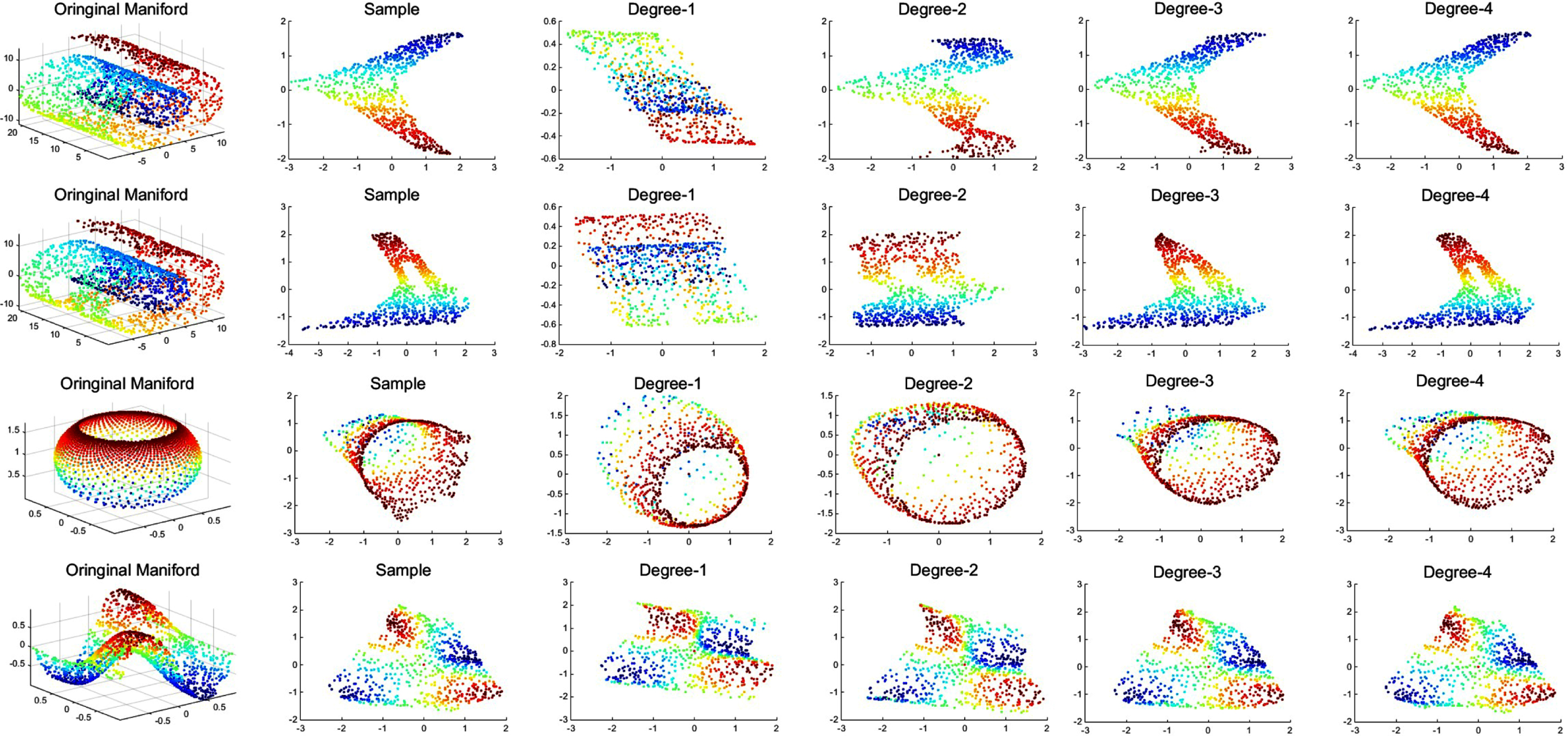
Polynomial approximation to LLE (K=10).

Fig. 2

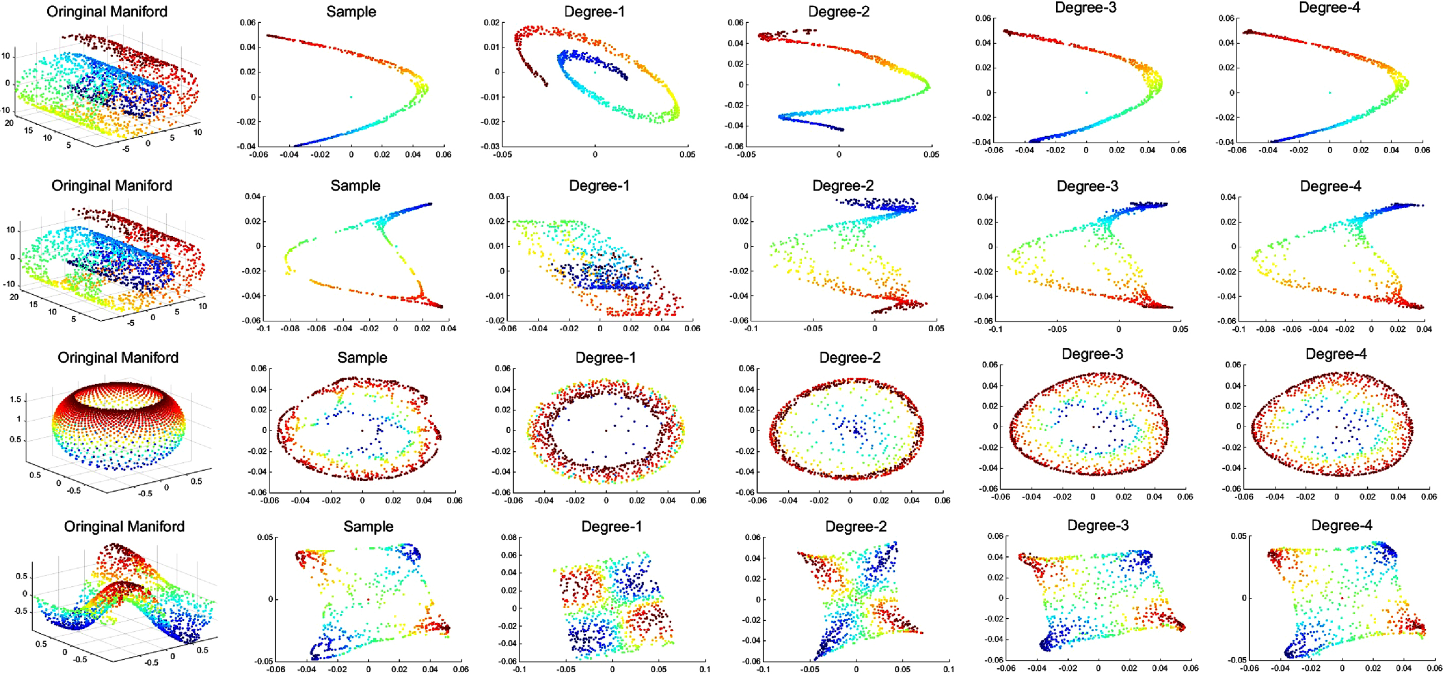
Polynomial approximation to LE (K=8).

Fig. 3

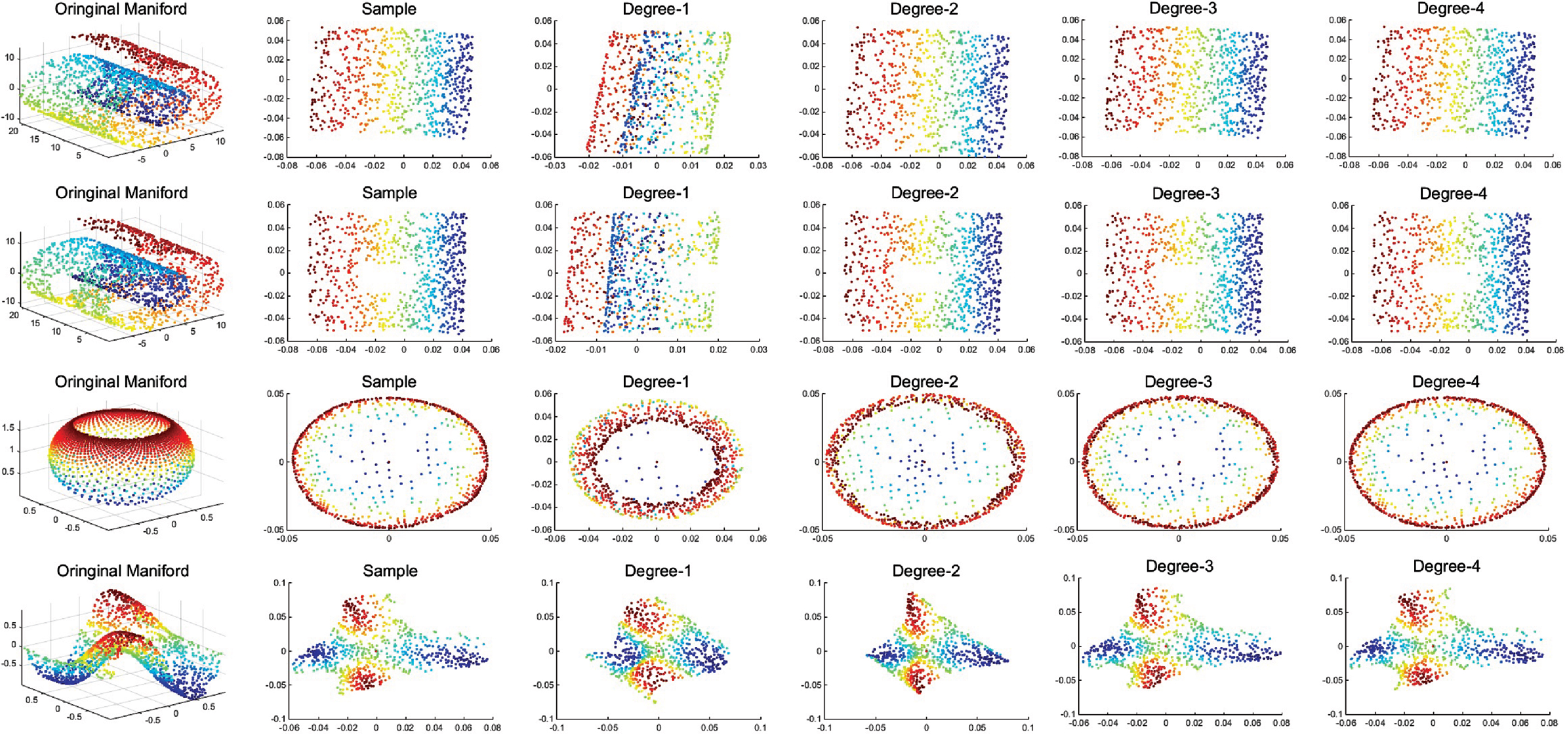
Polynomial approximation to LTSA (K=12).

Fig. 4

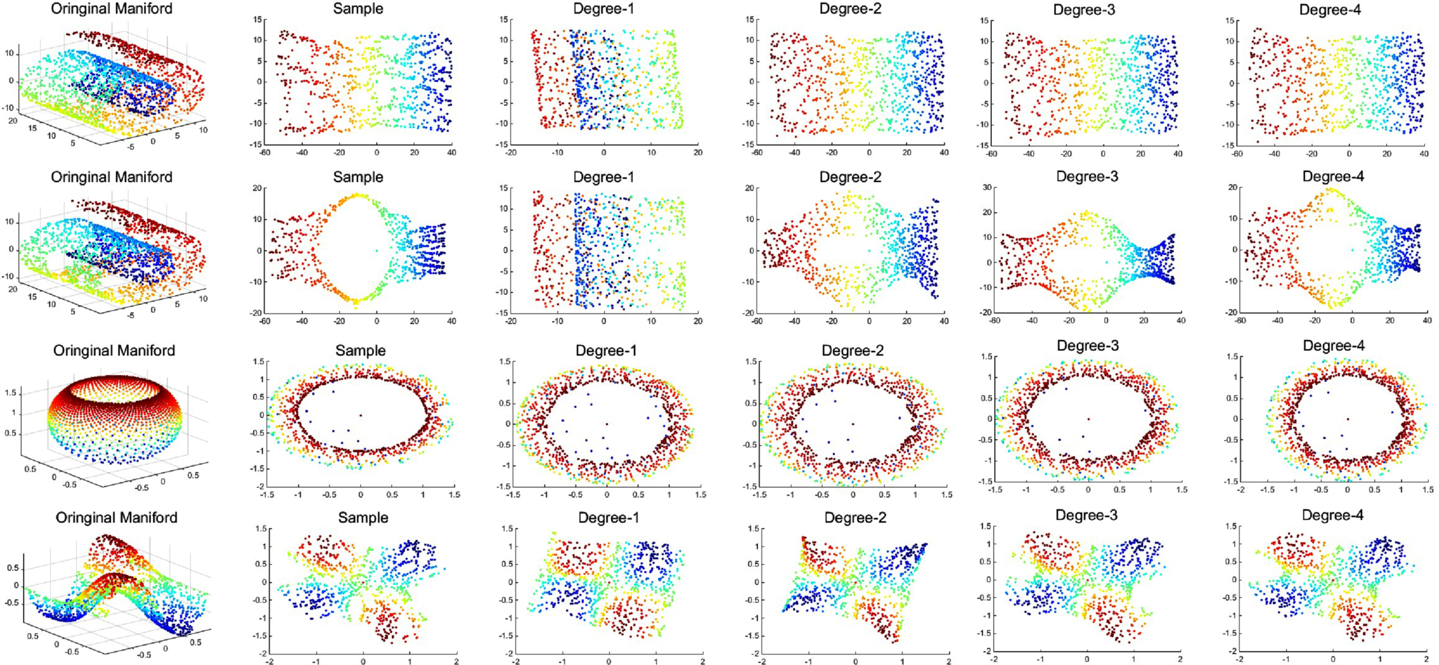
Polynomial approximation to ISOMAP (K=10).

4.2 Experiments of classification

In the section, to further demonstrate the approximation effect of PAML algorithm, we conduct classification experiments with the two manifold learning algorithm (LE, and LTSA) on the real data: Vehicle [34]. The vehicle data set is composed of 846 images of four vehicle models: double deck bus, saab9000, Chevrolet van and Opel Manta 400. Each vehicle image extracts 18 different attributes. Four vehicle models are the four classes of the data set, each of which has about 200-300 vehicle pictures.

In the experiments, 440 images in the data set are randomly selected as the training set, 320 images are randomly selected as test set. Each image is 18 dimensions. We apply our PAML with order 1∼4 on the test set and obtain the 2∼ 17-dimensionality reduction results. Furthermore, the KNN method is applied on the results for showing the accuracy of approximation of the proposed PAML. In Fig. 5 and Fig. 6), the purple line represent the classification result of the corresponding manifold learning algorithm, the other four line represent the result of PAML with order 1∼4. In each algorithm, first-order PAML has a lowest accuracy, and PAML with order 2∼4 have a close result with the corresponding manifold learning algorithm. It also means that our proposed PAML has the effective and optimal approximation to manifold learning.

Fig. 5

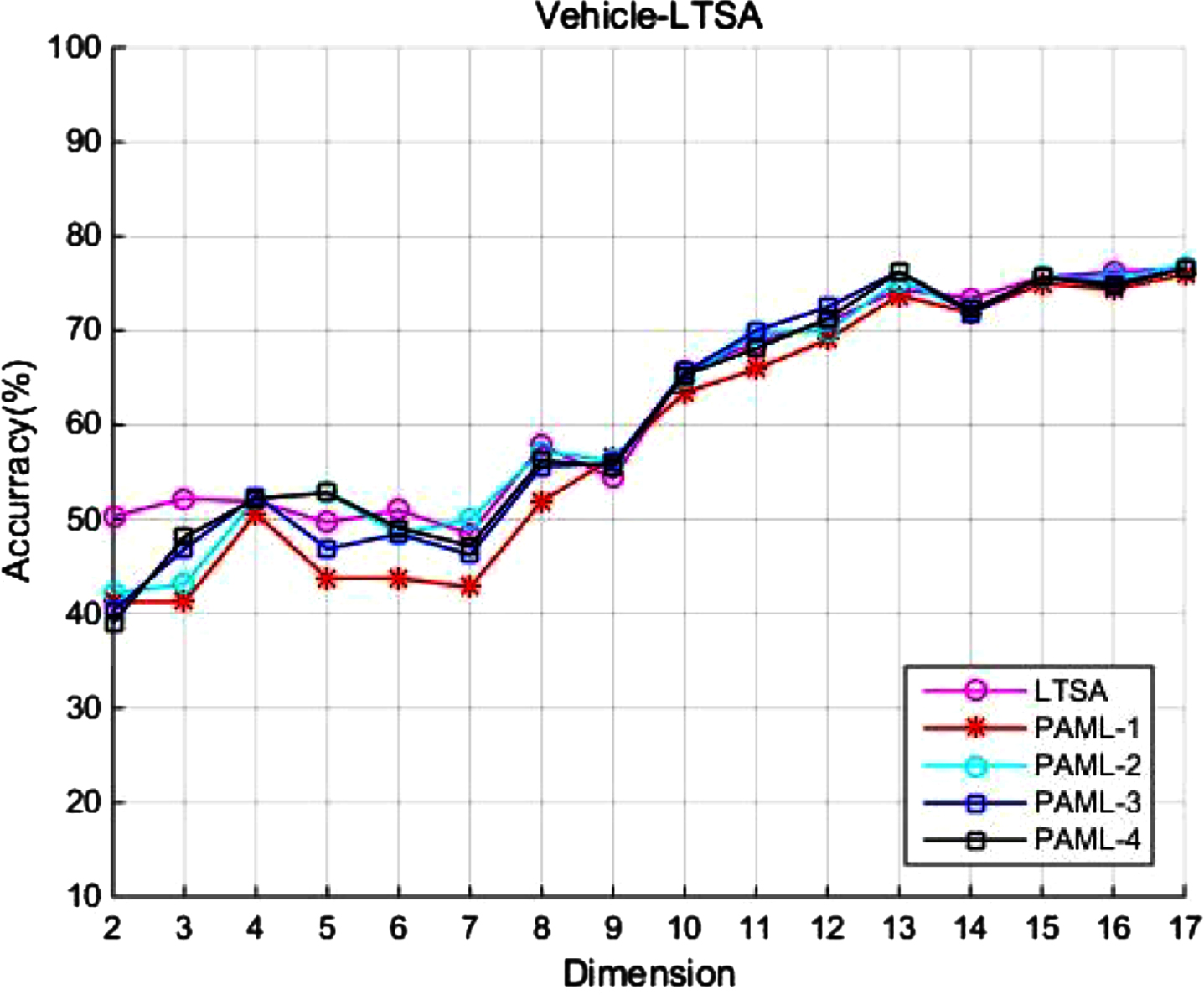
Classification experiments of LTSA and PAML with different order on the Vehicle dataset.

Fig. 6

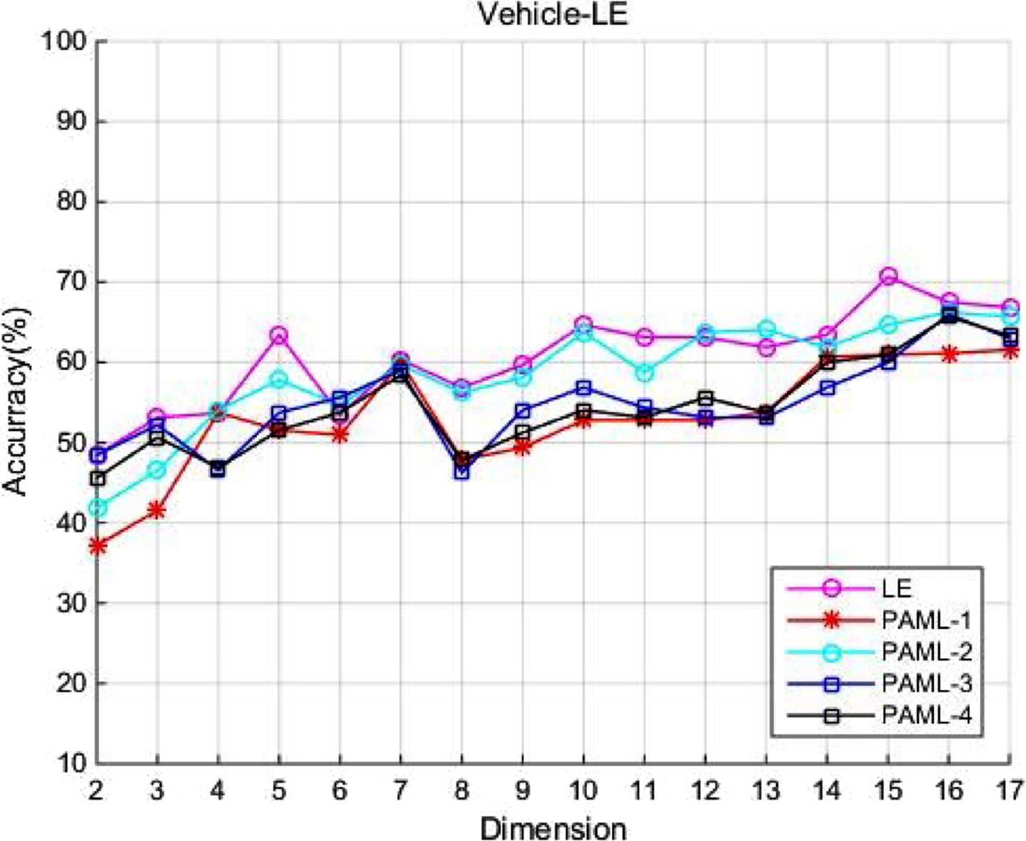
Classification experiments of LE and PAML with different order on the Vehicle dataset.

4.3 Experiments on out-of-sample

In the section, we conduct experiments on out-of-sample. We firstly compare our PAML with two manifold learning algorithms (LE, and LTSA) on four toy-data sets (Swiss roll, Swiss roll with hole, punctured sphere, and Gaussian) to show the dimension reduction expansion of new data. Secondly, we compare the proposed PMAL with four other algorithms (SC, LVM, KAML, SNPPE) proposed recent year to solve out-of-sample problem on four real-data sets (COIL, USPS, minst, Binary).

4.3.1 Experiment on Toy-data

In the experiments, the proposed PAML is firstly trained by 1000 toy-data, and then is applied on 150, 300, 450 out-of-sample points. On the other hand, we add the out-of-sample to the original training set and apply manifold learning algorithm on it to obtain the low-dimensional representation of data.

The experiments results are showed in Figs. 8. The above experiments show that the proposed PAML with order two already achieves a good result on some data sets. And some other data sets require third-order PAML.

Fig. 7

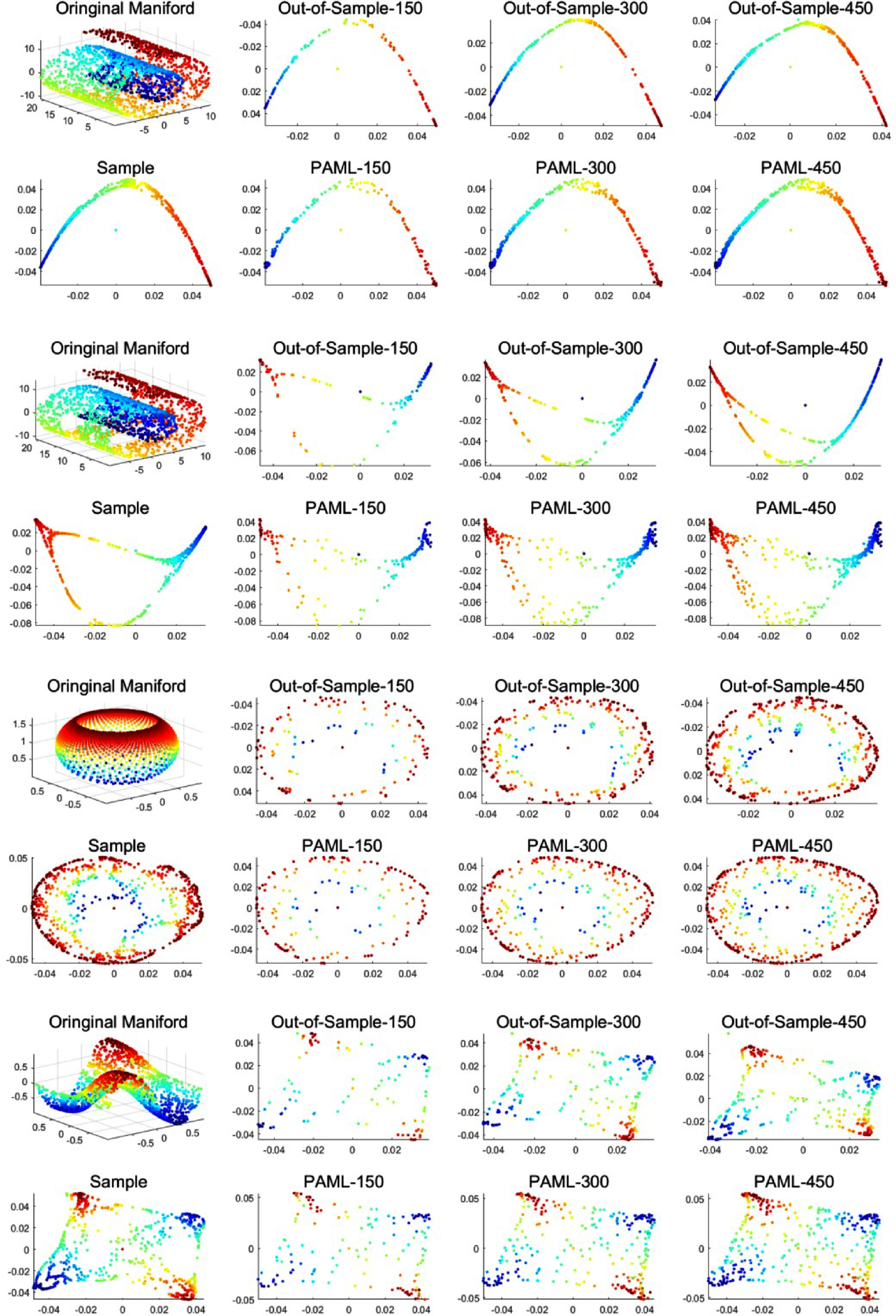
Dimensional reduction experiments of LE and PAML with different number of out-of sample.

Fig. 8

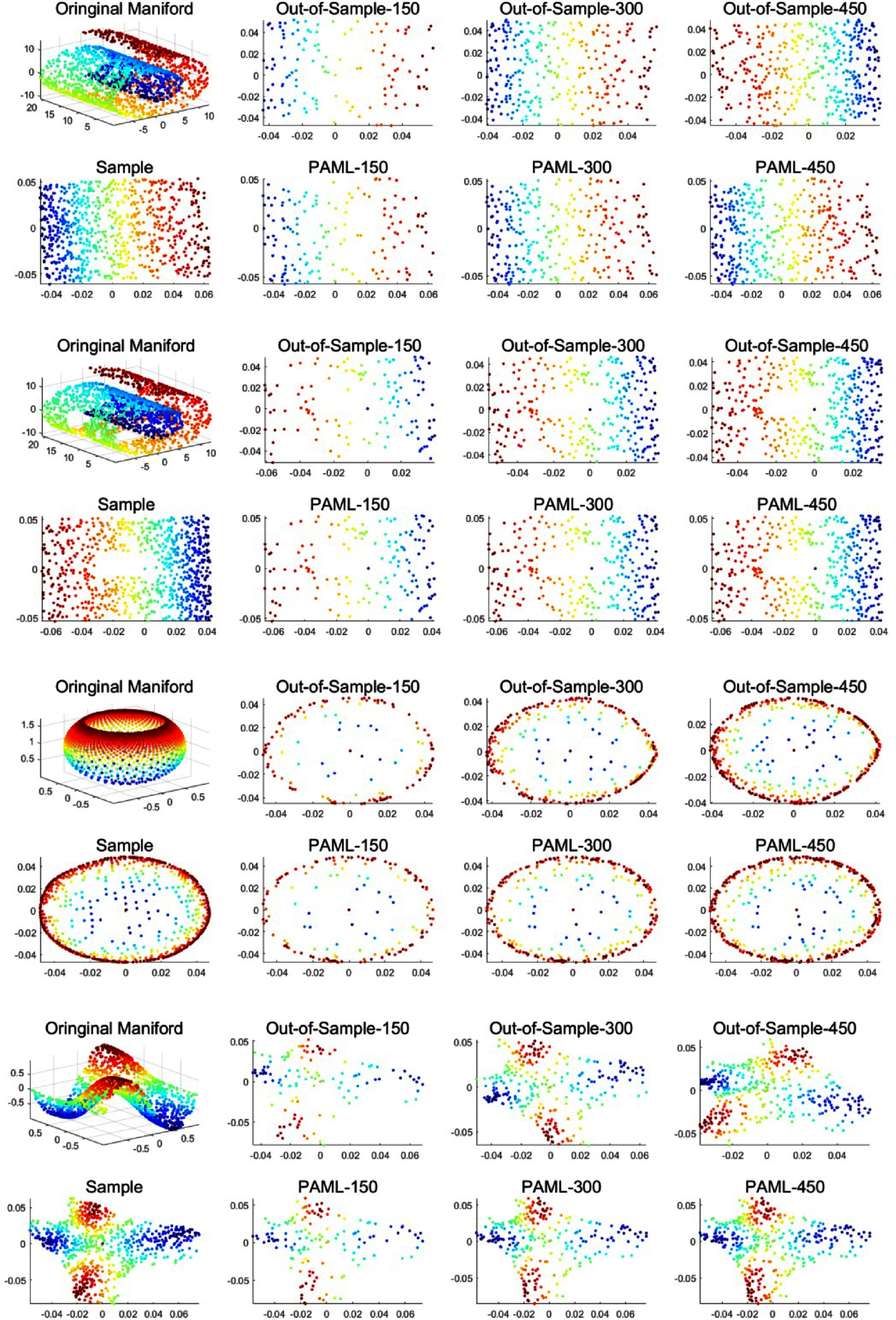
Dimensional reduction experiments of LTSA and PAML with different number of out-of sample.

According to the experimental results, the low dimensional results of new data set obtained by the PAML algorithm and the manifold learning algorithm are basically the same. It proves that the PAML algorithm proposed in this paper can effectively solve the problem of dimension reduction of new data.

4.3.2 Experiment on real-data

To get a get a more convincing compared result, the kernel method proposed by Vural and Guillemot [21] is put into the framework of this paper and name it KAML. Table. 1 shows the compared algorithm and their brief descriptions. The experiments are carried on the COIL [35] data set, the USPS data set (US Postal handwriting digit data-set: pictures 0∼9) [36], the mnist data set [37] (National Institute of Standards and Technology handwriting digit data-set: picture 0∼9), the Binary data [38] (handwriting digit dataset: picture 0∼9, A∼Z) (see Table 2). The training set and the test set (out-of-sample) are selected randomly, and then the manifold learning algorithm (LE or LTSA) is applied to find out the low-dimensional result of training set on different target dimension. The training set and its low-dimensional representation are used to train our PAML. Then we apply the trained PAML on the out-of-sample data and get the low-dimensional results of new data.

Table 1
The description of compared algorithms

Method Description

SC Application of sparse representation to dimension reduction of out-of-sample data.

LVM Dimension reduction algorithm combining latent variable model and feature mapping.

KAML Nonlinear manifold learning dimension reduction algorithm based on kernel space.

SNPPE Dimension reduction algorithm based on local polynomial hypothesis and manifold learning.

Method	Description
SC	Application of sparse representation to dimension reduction of out-of-sample data.
LVM	Dimension reduction algorithm combining latent variable model and feature mapping.
KAML	Nonlinear manifold learning dimension reduction algorithm based on kernel space.
SNPPE	Dimension reduction algorithm based on local polynomial hypothesis and manifold learning.

Table 2

The parameter of the four real-data sets

Dataset	Num.	Cluster	Dimension	Training set	Test set
COIL	1300	20	256	800	500
USPS	2000	10	256	1000	1000
mnist	1300	10	256	800	500
Binary	1404	36	320	864	540

Seen from the Tables 4, the LVM algorithm has a very low classification accuracy on the COIL data set. It means that the LVM algorithm is invalid on the COIL data set. The classification accuracy of the PAML algorithm proposed in this paper is close to the dimensionality reduction result of the manifold learning. At the low dimensions (2-40 dimensions), the classification accuracy of the SC algorithm and the PAML algorithm are slightly higher than that the SNPPE algorithm. And the classification accuracy of these three algorithms are higher than the KAML algorithm. Therefore, the algorithm proposed in this paper can be effectively used for dimensionality reduction of new data. And the classification accuracy of the PAML is close to the results of manifold learning algorithm.

Table 3

Classification accuracy on the COIL dataset(LTSA) (%)

Dim.	LTSA	PAML	KAML	SC	LVM	SNPPE-LTSA
2	48.2	15.2	11.2	25.0	6.0	21.6
5	84.6	54.4	31.8	68.2	5.0	60.0
10	90.6	82.6	57.0	83.2	5.0	74.6
20	86.6	88.6	68.0	88.4	5.0	82.2
30	93.4	75.8	60.0	82.4	5.0	84.0
40	96.0	96.8	93.2	96.0	5.0	88.2
50	95.0	97.2	93.4	96.8	5.0	89.6
60	96.0	97.2	91.8	96.0	5.0	89.4
80	95.6	96.8	86.6	95.8	5.0	89.2
100	95.8	95.6	77.4	94.6	5.0	91.0
Average	88.2	80.0	67.0	82.6	5.1	77.0

Table 4

Classification accuracy on the COIL dataset(LE) (%)

Dim.	LE	PAML	KAML	SC	LVM	SNPPE-LE
2	50.0	15.8	14.6	20.8	5.4	25.2
5	81.8	71.2	39.0	74.2	5.0	54.0
10	84.0	80.4	56.6	81.2	5.0	75.8
20	85.6	86.4	84.8	88.0	5.0	84.8
30	86.6	88.8	88.6	90.2	5.0	85.0
40	91.2	90.0	85.2	91.8	5.0	90.0
50	89.0	89.9	84.0	91.2	5.0	91.4
60	88.8	86.4	83.4	89.0	5.0	91.6
80	86.8	85.8	81.6	88.6	5.0	92.0
100	81.8	83.6	79.8	87.6	5.0	91.0
Average	82.6	77.8	67.0	80.2	5.0	78.1

Seen from the Tables 6, the PAML algorithm proposed in this paper almost has the highest classification accuracy among the five newly added data dimensionality reduction algorithms (PAML, KAML, SC, LVM and SNPPE). The proposed PAML is the closest to the dimensionality reduction effect of LTSA or LE, seen from the first column of the Table 5 and Table 6, respectively. In the lower dimensions (2-40 dimensions), the SC algorithm and the proposed PAML have more higher classification accuracy than the SC algorithm, and the classification accuracy of these three algorithms are higher than the SNPPE algorithm. It means that the PAML algorithm proposed in this paper is effective in the dimensionality reduction applications of the new data.

Table 5

Classification accuracy on the USPS dataset(LTSA) (%)

Dim.	LTSA	PAML	KAML	SC	LVM	SNPPE-LTSA
2	56.1	38.0	28.7	30.1	41.8	16.2
5	70.2	55.2	44.7	46.0	46.4	28.3
10	84.3	78.2	76.0	74.8	69.8	39.8
20	86.3	84.2	83.4	82.0	78.2	48.8
30	87.9	82.5	82.6	84.6	77.4	58.2
40	86.8	81.3	74.5	83.8	71.7	62.9
50	84.1	77.5	64.3	80.4	60.9	67.3
60	82.1	73.8	53.9	76.3	46.7	69.2
80	75.7	65.0	30.6	68.7	26.7	72.5
100	64.3	55.4	23.0	60.7	18.2	72.8
Average	77.8	69.1	56.2	68.7	53.8	53.6

Table 6

Classification accuracy on the USPS dataset(LE) (%)

Dim.	LE	PAML	KAML	SC	LVM	SNPPE-LE
2	57.9	42.3	35.1	36.3	34.5	15.3
5	75.8	61.0	46.5	47.5	50.9	22.1
10	80.1	76.5	73.7	69.2	63.7	33.7
20	82.9	79.1	76.5	72.6	71.2	45.9
30	84.0	79.7	72.6	70.8	70.9	54.8
40	83.7	79.5	68.5	72.1	67.2	57.6
50	82.4	77.4	67.2	69.4	65.5	59.4
60	81.9	76.3	67.9	69.5	65.8	65.0
80	80.2	76.3	72.0	69.9	66.8	68.0
100	76.9	76.7	74.3	70.5	68.1	69.5
Average	78.6	72.5	65.4	64.8	62.5	49.1

Seen from the Table 7 and Table 8, the proposed PAML algorithm almost has the highest classification accuracy among the five compared algorithms. And it also is close to the manifold learning algorithm (LTSA or LE), seen from the first column of the Table 7 and Table 8. It means that the PAML algorithm proposed in this paper is an optimal approximation to the manifold learning algorithm, and has effective performance in the applications of the dimensionality reduction of the new data.

Table 7

Classification accuracy on the mnist dataset (LTSA) (%)

Dim.	LTSA	PAML	KAML	SC	LVM	SNPPE-LTSA
2	61.9	51.8	35.5	42.9	15.5	44.7
5	72.5	63.9	51.8	53.8	24.4	55.4
10	84.0	82.2	76.4	74.2	36.5	72.7
20	86.8	85.0	85.0	82.3	55.0	82.6
30	88.0	85.7	87.7	83.2	59.0	76.0
40	87.7	84.1	86.7	82.1	65.5	71.3
50	86.8	82.2	84.8	81.3	68.0	61.7
60	83.5	80.4	80.2	78.2	72.4	60.0
80	79.8	76.1	71.5	73.3	74.7	59.4
100	74.2	72.1	62.1	67.4	76.5	58.3
Average	80.5	76.4	72.2	71.9	54.8	64.2

Table 8

Classification accuracy on the mnist dataset (LE) (%)

Dim.	LE	PAML	KAML	SC	LVM	SNPPE-LE
2	63.5	52.2	41.1	44.8	17.0	20.2
5	80.1	70.4	63.0	62.8	26.4	28.1
10	84.3	78.8	75.9	69.8	38.1	41.5
20	83.9	82.7	80.8	75.8	57.2	56.9
30	83.7	82.1	82.6	77.2	59.0	58.1
40	84.8	82.5	83.1	76.5	66.0	64.4
50	84.1	82.4	84.0	78.0	68.7	67.2
60	84.6	82.5	84.2	78.4	72.4	70.2
80	82.3	82.3	83.2	76.7	74.9	70.8
100	82.4	79.2	82.2	75.8	76.5	73.8
Average	78.6	72.5	65.4	64.8	62.5	49.1

Tables 10 are the experimental results of classification of six compared algorithms on the Binary data set. It can be seen that the proposed PAML algorithm almost has the highest classification accuracy. In particular, the classification accuracy of the SNPPE and the LVM are very low. It proves that our PAML algorithm has an optimal approximation to the manifold learning, and has effective performance in the applications of the dimensionality reduction of the new data.

Table 9

Classification accuracy on the Binary dataset (LTSA) (%)

Dim.	LTSA	PAML	KAML	SC	LVM	SNPPE-LTSA
2	30.6	20.9	13.7	11.7	7.8	4.2
5	53.3	41.9	24.8	22.0	12.2	2.6
10	58.5	56.9	41.3	39.1	25.7	3.3
20	64.6	63.2	56.1	55.9	27.6	2.2
30	65.7	61.3	56.9	57.8	26.5	4.4
40	63.7	60.0	53.7	55.0	19.8	4.4
50	62.4	55.6	47.0	56.7	9.4	3.9
60	55.4	51.5	46.1	55.6	8.5	4.3
80	52.0	44.6	40.6	49.1	10.2	3.7
100	41.3	39.3	35.4	36.5	10.4	2.6
Average	54.8	49.5	41.6	43.9	15.8	3.6

Table 10

Classification accuracy on the Binary dataset (LE) (%)

Dim.	LE	PAML	KAML	SC	LVM	SNPPE-LE
2	35.2	21.5	12.2	10.0	9.8	3.0
5	49.1	40.2	22.9	24.1	15.7	3.5
10	54.3	51.1	37.4	35.4	17.9	4.1
20	55.7	57.2	41.7	41.3	16.7	5.6
30	57.9	57.0	35.6	38.9	14.1	4.6
40	58.7	53.3	32.0	37.6	12.0	5.9
50	58.7	52.9	33.5	35.9	11.8	5.2
60	57.0	50.9	33.9	35.7	11.1	5.6
80	54.3	50.0	34.6	34.0	9.4	5.6
100	53.2	48.0	33.9	33.9	8.9	5.2
Average	53.4	48.2	31.8	32.7	12.8	4.8

In summary, the proposed PAML almost has the highest dimensionality reduction accuracy on the USPS dataset, the MNIST, and the Binary dataset, and also has an effective performance on the COIL dataset. And in most case, the average dimensionality reduction accuracy of the PAML is the highest. Particularly, in some lower dimension results, the proposed PAML still demonstrates the good results. The LVM algorithm and KAML algorithm have an efficiency performance on the COIL dataset. But they have a large number of parameters to be adjusted. The KAML algorithm can achieve a good dimensionality reduction result when the parameters are adjusted properly. However, the parameter adjustment requires lots of time cost. The SNPPE algorithm also needs the proceeding of neighborhood parameters selecting for better dimensionality reduction effects. The SC algorithm and the proposed PAML algorithm can avoid the parameter adjustment. But the SC algorithm is not suitable for large amounts of data processing. The proposed PAML algorithm can effectively apply to the dimensionality reduction of large-scale data when the dimensionality of result is not too high.

5 Conclusions

Manifold learning is an very important component of nonlinear dimensionality reduction. Even the surveys of dimensionality reduction methods must describe the manifold learning algorithms in detail. The most important characteristics of manifold learning algorithms are the locality and the nonlinearity. The locality characteristic means that the manifold learning algorithms explore the local nature of manifold dataset by decomposing it into patches (except ISOMAP) and learning their local Homeomorphism. And manifold learning algorithms obtain the nonlinear dimensionality reduction results of data, which is the manifold learning prides itself. However, many classical manifold learning cannot give an explicit expression relationship between the high-dimensional data and its low-dimensional representation. Therefore, it cannot effectively handle the out-of-sample problem. For new data, these methods often need to add them to the original data set for retraining their models. Whatever the number of new data is small or large, it is both uneconomical and inefficient. In recent, some improved methods for out-of-sample are proposed, which usually introduce an fixed linear or nonlinear mapping to the object function of manifold learning. Actually, these methods damage the intrinsic structure of manifold. Because the fix mapping establishes an global relationship between the low- and high-dimensional data, not reflecting the locality of manifold. For example, the LLP algorithm introduces the fix linear mapping to the LE algorithm for new data, which in essence is a linear dimensional reduction method. Strictly speaking, although these improved algorithms are constructed based on manifold learning, they are no longer be regarded as manifold learning algorithms from the view of methodology. The dimensionality reduction of data, regardless of the explicit or implicit relationship, is to establish a functional relationship between the high- and low-dimensional data.

In mathematics, any continuous function can be infinitely approximated by polynomials. Inspired by it, we propose a novel manifold learning algorithm based on polynomial approximation, which learns the polynomial approximation of manifold learning by using the dimensionality reduction results of manifold learning and the original high-dimensional data. The accuracy of polynomial approximation can be adjusted by adjusting the order of the polynomials. And with this polynomial approximation, the problem of out-of-sample can be easy solved. Our PAML does not change the objective function of manifold learning, i.e., is a true manifold learning algorithm. Finally, we conduct adequate experiments on four toy-data sets and five real-world data sets with four classical manifold learning algorithms and some state-of-the-art algorithms to demonstrate the effectiveness of the proposed method.

Footnotes

Acknowledgment

This work is supported in part by the Guangdong Basic and Applied Basic Research Foundation under Grant 2019A1515111143 and by the Natural Science Foundation of China under Grant 62006042.

References

Lin

and Zha

Riemannian manifold learning, IEEE Transactions on Pattern Analysis and Machine Intelligence 30(5) (2008), 796–809.

Raducanu

and Dornaika

Embedding new observation via sparse-coding for non-linear manifold learning, Pattern Recognition 47(1) (2014), 480–492.

Zhang

, Huang

, et al. Manifold learning for visualizing and analyzing high dimensional data, IEEE Intelligent Systems 25(4) (2010), 54–61.

Trosset

M.W.

and Priebe

C.E.

The out-of-sample problem for classical multi-dimensional scaling, Computational Statistics and Data Analysis 52(10) (2008), 4635–4642.

Tenenbaum

J.B.

, Silva

V.D.

, et al., A global geometric framework for nonlinear dimensionality reduction, Science 290 (2000), 2319–2323.

Borg

and Groenen

Modern multi-dimensioanal scaling: theory and applications, Journal of Educational Measurement 40(3) (2003), 277–280.

Roweis

and Saul

Nonlinear dimensionality reduction by locally linear embedding, , Science 290 (2000), 2323–2326.

Zhang

and Zha

Principal manifold and nonlinear dimensionslity reduction via tangent space alignment, SAIM Journal on Scientific Computing 26(1) (2004), 313–338.

Belkin

and Niyogi

Laplacian eigenmaps for dimensionality reduction and data representation, Neural Computation 15(6) (2003), 1373–1396.

10.

Elganmmal

and Lee

Nonlinear manifold learning for dynamic shape and dynamic appearance, Computer Vision and Image Understanding 106(1) (2007), 31–46.

11.

Yang

, Nie

, et al., Local and global regressive mapping for manifold learning with out-of-sample extrapolation, AAAI Conference on Artificial Intelligence, AAAI Press, 2010, 649–654.

12.

Piret

Analytical and numerical advances in radial basis functions, University of Colorado at Boulder, 2007.

13.

Scheuerer

An alternative procedure for selecting a good value for the parameter c in RBF-interpolation, Advances in Computational Mathematics 34(1) (2011), 105–126.

14.

Dollar

, Rabaud

, et al., Learning to traverse image manifolds, Conference on Advances in Neural Information Processing Systems, 2007.

15.

Verbeek

Learning nonlinear image manifold by global alignment of local linear models, IEEE Transactions on Pattern Analysis and Machine Intelligence 28(8) (2006), 1236–1250.

16.

Strange

and Zwiggelaar

A generalised solution to the out-of-sample extension problem in manifold learning, AAAI Conference on Artificial Intelligence, AAAI Press, 2011, 471–476.

17.

Raducanu

and Dornaika

Embedding new observation via sparse-coding for non-linear manifold learning, Pattern Recognition 47(1) (2014), 480–492.

18.

Bengio

, Paiement

, et al., Out-of-sample extensions for LLE, ISOMAP, MDS, Eigenmaps, and Spectral Clustering, International Conference on Neural Information Processing Systems, 2003.

19.

Chin

and Suter

Out-of-sample extrapolation of learned manifolds, IEEE Transactions on Pattern Analysis and Machine Intelligence 30(9) (2008), 1547–1556.

20.

Aizenbud

, Bermanis

, et al., PCA-based out-of-sample extension for dimensionality reduction, Statistic Journal on Machine Learning, 2015.

21.

Vural

and Guillemot

Out-of-sample generalizations for supervised manifold learning for classification, IEEE Transactions on Image Processing 25(3) (2016), 1410–1424.

22.

Han

, Meng

, Xu

and Gu

Incremental alignment manifold learning, Journal of Computer Science and Technology 26(1) (2011), 153–165.

23.

Qiao

, Zhang

, Wang

and Zhang

A explicit nonlinear mapping for manifold learning, IEEE Transactions on Cybernetics 43(1) (2013), 51–63.

24.

Shuicheng

, Dong

, Benyu

and Hong-Jiang

Graph embedding and extensions: a general gramework for dimensionality reduction, IEEE Transactions on Pattern Analysis and Machine Intelligence 29(1) (2007), 40–51.

25.

Wang

Mathematical analysis on out-of-sample extensions, International Journal ofWavelets Multiresolution and Information? Processing, 2018.

26.

Yan

and Wang

Semi-supervised learning by sparse representation, SIAM International Conference on Data Mining, 2009.

27.

Carreira-Perpinan

and Lu

The Laplacian eigenmaps latent variable model, Journal of Machine Learning Research 2 (2007), 59–66.

28.

and Niyogi

Locality preserving projections, Advance in Neural Information Processing Systems, 2003.

29.

, Yan

, et al., Face recognition using laplacianfaces, IEEE Transactions on Pattern Analysis and Machine Intelligence 27(3) (2005), 328–340.

30.

, Cai

, et al., Neighborhood preserving embedding,, ICCV Press, , International Conference on Computer Vision 2 (2005), 1208–1213.

31.

Pang

, Zhang

, et al., Neighborhood preserving projections (NPP): A novel linear dimension dimension reduction method, International Conference on Computer Science, ICIC Press, 2005, 117–125.

32.

Vural

and Guillemot

, A study of the classification of low-dimensional data with supervised manifold learning, British Journal of Sociology, 2018.

33.

http://www.math.ucla.edu/ wittman/mani.

34.

http://iitlab.bit.edu.cn/mcislab/vehicledb/.

35.

http://www.cs.columbia.edu/CAVE/software/softlib/coil-20.php.

36.

available: http://www.cs.nyu.edu/roweis/data.html.

37.

http://yann.lecun.com/exdb/mnist/.

38.

https://cs.nyu.edu/ roweis/data.html.

39.

Keyhannian

and Nasersharif

, Laplacian eigenmaps latent viriable model modification for Pattern Recognition International Conference on Electrical Engineering, ICEE Press, 2015, 668–673.

40.

Weinberger

and Saul

, Unsupervised learning of image manifolds by semidefinite programming, International Journal of Computer Vision 70(1) (2006), 77–90.