A structure-protecting kernelized semi-supervised space adjustment for classification

Abstract

We introduce a semi-supervised space adjustment framework in this paper. In the introduced framework, the dataset contains two subsets: (a) training data subset (space-one data (SOD)) and (b) testing data subset (space-two data (STD)). Our semi-supervised space adjustment framework learns under three assumptions: (I) it is assumed that all data points in the SOD are labeled, and only a minority of the data points in the STD are labeled (we call the labeled space-two data as LSTD), (II) the size of LSTD is very small comparing to the size of SOD, and (III) it is also assumed that the data of SOD and the data of STD have different distributions. We denote the unlabeled space-two data by ULSTD, which is equal to STD - LSTD. The aim is to map the training data, i.e., the data from the training labeled data subset and those from LSTD (note that all labeled data are considered to be training data, i.e., SOD ∪ LSTD) into a shared space (ShS). The mapped SOD, ULSTD, and LSTD into ShS are named MSOD, MULSTD, and MLSTD, respectively. The proposed method does the mentioned mapping in such a way that structures of the data points in SOD and MSOD, in STD and MSTD, in ULSTD and MULSTD, and in LSTD and MLSTD are the same. In the proposed method, the mapping is proposed to be done by a principal component analysis transformation on kernelized data. In the proposed method, it is tried to find a mapping that (a) can maintain the neighbors of data points after the mapping and (b) can take advantage of the class labels that are known in STD during transformation. After that, we represent and formulate the problem of finding the optimal mapping into a non-linear objective function. To solve it, we transform it into a semidefinite programming (SDP) problem. We solve the optimization problem with an SDP solver. The examinations indicate the superiority of the learners trained in the data mapped by the proposed approach to the learners trained in the data mapped by the state of the art methods.

Keywords

Semi-supervised domain adaptation non-linear optimization local-preserving domain adaptation semidefinite programming kernel learning principal component analysis

1 Introduction

In almost all of the classic learning algorithms in artificial intelligence, the hidden assumption is a proposition that distributions of the training and the testing instances are identical; i.e., the training and the testing spaces are the same. However, there are some problems in which this proposition is not correct. In this condition, we face a special type of transfer learning [52 –56] (TL) called transductive transfer learning. We use a space adjustment (SA) approach to deal with transductive transfer learning (see Fig. 1). Therefore, space adjustment (SA) can be considered to be a subfield in transductive transfer learning.

Fig. 1

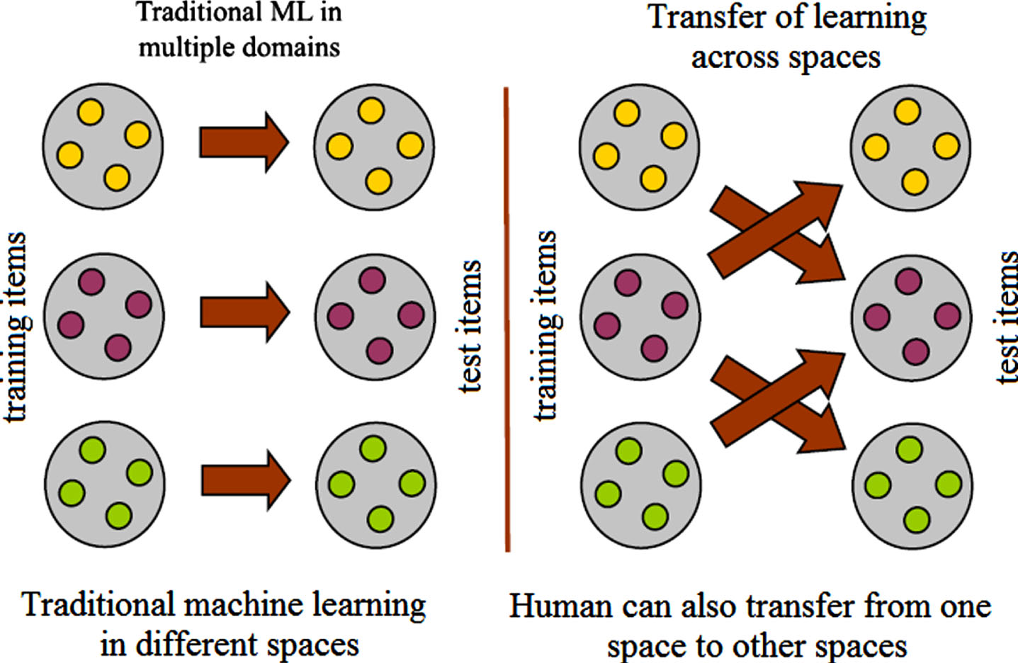
Simple learning systems (left), SA learning systems (right).

Indeed, any learning algorithm in artificial intelligence belongs to one of the following four learning types: (a) simple traditional learning in which both of the training data and testing data are of the same distribution (for example when we use some Chinese facial imagery samples as positive training samples of face class against non-facial imagery samples as negative training samples, and then we use some other Chinese facial imagery samples as positive testing samples against some other non-facial imagery samples as negative testing samples), (b) transductive transfer learning in which the training data and testing data are not of the same distribution (for example when we use some Chinese facial imagery samples as positive training samples of face class against non-facial imagery samples as negative training samples, and then we use some non-Chinese facial imagery samples as positive testing samples against some other non-facial imagery samples as negative testing samples), (c) inductive transfer learning in which the training data and testing data are of the same distribution, but testing data is about another task different from the task of training data (for example when we use some Chinese facial imagery samples as positive training samples of face class against non-facial imagery samples as negative training samples, and then we use some other imagery samples of Chinese passengers containing facial contents as positive testing samples against some other imagery samples that do not contain anybody as negative testing samples; i.e. we want to use the learnt model to detect Chinese passengers in images), and (d) unsupervised transfer learning in which both of the training data and testing data are not of the same distribution, and also testing data is about another task different from the task of training data (for example when we use some Chinese facial imagery samples as positive training samples of face class against non-facial imagery samples as negative training samples, and then we use some other imagery samples of non-Chinese passengers containing facial contents as positive testing samples against some other imagery samples that do not contain anybody as negative testing samples; i.e. we want to use the learnt model to detect non-Chinese passengers in images).

An example among SA applications is the one in which we have temporal data with a limited time of validation. In such an application, an old expert model (trained on previous expired data) can be still useful if a transfer learning or a space adjustment is done; otherwise, a new model should be retrained from the scratch on currently-valid data. It is clear that an existent concept (or a learned model) may be changed after a while, but the old concept can still be useful in the definition of its modern concept. For example, Cathode Ray Television (CRT) was the first concept shaped in the mind of a human A as a Television. Now, the CRT is no longer the representative of a Television concept, but the human A does not try to learn the modern Television concept from scratch. He tries to learn it by extending the CRT concept. The extension of the CRT concept to a modern Television concept is called SA (see Fig. 1).

From another perspective, the SA approaches can be divided into three partitions:

Supervised: in which some of the training instances are from the testing data distribution (for example, if we use some Chinese facial imagery samples as positive training samples of face class against non-facial imagery samples as negative training samples and use some non-Chinese facial imagery samples as positive testing samples against some other non-facial imagery samples as negative testing samples, we may add some non-Chinese faces to our training samples).

SemiSupervised: in which there are a number of the unlabeled training instances that are from the testing data distribution, and there are also a number of the labeled training instances that are from the testing data distribution.

Unsupervised: in which there are a number of the unlabeled training instances that are from the testing data distribution.

Our proposed method is of the second type, i.e., SemiSupervised SA. Indeed, we introduce a SemiSupervised SA framework as our proposed method. In the introduced framework, the dataset contains two subsets: (a) training data subset (space-one data (SOD)) and (b) testing data subset (space-two data (STD)). The unsupervised space adjustment framework learns under three assumptions: (I) it is assumed that all data points in the SOD are labeled, and only an insignificant fraction of data points in the STD are labeled (we call the labeled space-two data as LSTD), (II) the size of LSTD is very small comparing to the size of SOD, and (III) it is also assumed that the data points in SOD and the data points in STD have different distributions. We denote the unlabeled space-two data by ULSTD, which is equal to STD - LSTD. The aim is to map the training data, i.e., the data from the training data subset and LSTD (all labeled data are considered to be training data, i.e., SOD ∪ LSTD) into a shared space (ShS). The data points in SOD, STD, ULSTD, and LSTD after mapping into ShS are respectively named MSOD, MSTD, MULSTD, and MLSTD. The proposed method does the mentioned mapping in such a way that structures of the data points in SOD and MSOD, those in STD and MSTD, those in ULSTD and MULSTD, and those in LSTD and MLSTD are the same. In the proposed method, the mapping is done by a linear transformation on kernelized data. In the proposed method, it is tried to find a mapping that (a) can maintain the neighbors of data points after the mapping (i.e., while our method tries the closest instances to any arbitrary instance in SOD to be the same as the closest instances to that arbitrary instance in MSOD, it does the task in a non-parametrical manner, and this can be considered to be its advantage rather than a similar work proposed by Pan et al. [1], in which a couple of parameters are required) an) can integrate the concepts (classes) in SOD during transformation (the concepts defined according to the real labels in the SOD and the STD). After that, the problem of finding the optimal mapping is formulated into a non-linear constrained objective function. To find an optimal solution to the mentioned non-linear constrained objective function, it is transformed into a semidefinite programming (SDP) problem. Then, this optimization problem is approximately solved by an SDP solver. The examinations indicate the superiority of the learners trained in the data mapped by the proposed approach to the learners trained in the data mapped by the state of the art methods.

The most similar work to the proposed work in this paper is TCA (Transfer Component Analysis) [1]. However, TCA is an unsupervised SA framework, while our approach is a SemiSupervised SA framework. Meanwhile, both methods find the transformation matrix in the kernel space. Our contribution includes the defining of a SemiSupervised SA framework and its solving in a kernel space.

It may seem that it is a special case of a violation of the Independent and Identically Distributed (IID) assumption. It is worthy to note that this is what is referred to as either “Covariate Shift”, or “Model Drift”, or “Nonstationarity”, and so on [48] by Machine Learning society. Note that it cannot be referred to as IID violation; because it assumes a drift has occurred in a correctly learned concept. Indeed, it assumes that the model learned the concept correctly. However, the concept would change later ding the test phase. Therefore, it could be no longer valid.

In statistics, it is always aimed to reduce dataset sizes so as to its understanding and analysis can be easier. Solving multi-dimensional scaling (MDS) is a solution to this problem. MDS can be considered as a multi-variate data analysis task that transforms a dataset with high-dimensionality into a dataset with low-dimensionality. We are able to use a linear [22, 51] or a non-linear model for performing a given MDS task. While transforming a dataset into a new space, MDS tries to preserve local similarities [49]. The dataset, which is used as input of MDS, is transformed into a similarity (or a dissimilarity) matrix, also named input similarity matrix (ISM) or input dissimilarity matrix (IDM). The output dataset, after applying an MDS, has a similarity (or a dissimilarity) matrix, which is named output similarity matrix (OSM) or output dissimilarity matrix (ODM). The MDS task on a given dataset should be done in such a way that its ISM (or IDM) is equal to OSM (or ODM). While the MDS task is similar to our proposed problem, it is different from our problem because of the lack of any data object in the output space. Therefore, it is completely and fundamentally different from the topic of this paper.

The experimental studies are summarized in three subsections: (a) a subsection is dedicated to experiments on UCI repository datasets, (b) a subsection is dedicated to experiments on Land Mine datasets, and (c) a subsection is dedicated to experiments on office dataset. Considering the experimental studies, it can be inferred that the proposed method outperforms the recent baseline methods empirically.

In the residual of this manuscript, we present the literature review first. We introduce the problem statement and the proposed method in the subsequent section. We deal with the empirical study issue in Section 4. The conclusions of the paper and guidelines for future works are discussed in the last section, i.e., Section 5.

2 Literature review

Transfer learning in machine learning is a special type of learning in which the source domain/space (SD/SS) is different from the destination domain/space (DD/DS); for example, their features can be inherently different, or for another example, only their data distributions can be different [36]. Two main approaches emerge to deal with applications suffering from this problem: (a) employing a weighting strategy to determine the participation amount of each data point of the source domain/space in the learning task [37 –39], and (b) transforming the source domain/space and the destination domain/space into a shared domain/space [40 –43]. Each method that is based on the first approach is a member of instance-based methods (IBM) [6 –8], and each method that is based on the second approach is a member of feature-based methods (FBM) [3 , 9–12].

Multi-task learning (MTL) [40, 41], multi-domain learning (MDL) [45], domain adaptation (DA) [46], sample selection bias (SSB) (or co-variate shift (CVSh)) and self-taught learning (STL) [43] are among TL approaches.

DA as a subfield in TL is dealt with by natural language processing (NLP) [40 , 44] and sentiment classification [45]. Structural correspondence learning (SCL) is introduced [40, 42] as an FBM in DA. SSB methods like kernel mean matching (KMM) [38] and kullback-leibler (KL) importance estimation procedure (KLIEP) [39] are usually among IBM, and consequently, they are different from the proposed method. Although most of the DA methods are of IBM type, the proposed method is an example of FBM. The DA methods of the IBM type are usually unable to transfer a trained concept by matching the domains (or SA).

While methods of FBM type have been used in MTL [40, 41], MDL [42], and STL [43], there are only a few DA works of FBM type (like TCA [46] in DA). However, TCA is different from the proposed method because it is an unsupervised DA, while the proposed method is supervised. Our method, which makes a supervised space adjustment, can be considered to be a subfield in DA. It has been shown that the DA is applicable to different problems [4, 5].

Some related works in which SA are performed in a kernelized space have emerged recently [1 , 13–15]. Pan et al. [1] evaluate the kernel Gram matrices and learn an optimal sub-space in the kernelized space in which the distributions of the data points in the original and projected spaces are close to each other. Howard et al. [13] align the kernelized Gram matrices of original and test-data spaces in which the distributions of the data points in both original and projected spaces are forced to be similar in the Reproducing Hilbert Kernel Space (RHKS). Works done in [14, 15] explain a supervised SA approach in which a Support Vector Machine (SVM), which is trained on examples available from SOD, is transformed by adding a bias term between original and test-data spaces during optimization in the training phase.

Another topic close to the SemiSupervised SA is semi-supervised learning, in which there is a few labeled training samples [34]. While semi-supervised learning assumes that both (1) the training set of data points with labels and (2) the training set of data points without labels have the same distribution, the mentioned assumption does not hold in the SA. This is their only major difference.

Shi et al. introduce a method named Actively Transfer Domain Knowledge (ATDK), which actively selects some samples from STD to be labeled [16]. Their method is considered to be a supervised SA approach. Sugiyama et al. [6] propose a method to minimize the KL-divergence between SOD and STD by giving suitable weights to the examples. Weights are characterized as a linear model whose parameters are obtained using a convex optimization procedure. Pan et al. [1] calculated a transformation min the RHKS using kernelized Gram matrices of SOD and STD. A trace optimization problem was suggested to minimize the difference between distributions of SOD and STD, while maximally preserving the data variance and localities of the da. Like our proposed method, TCA calculates the transformation matrix in RHKS and projects the transformed SOD into a sub-space of the original RHKS. Saenko et al. [3, 10] propose a method that finds a transformation matrix such that the distances between examples in the same space are minimized while those between samples from different spaces are maximized. Applications of SA to enhance the results of object detection and video recognition can be considered to be some of the SA successful applications [3 , 17–21]. We compare the performance of our proposed method with the state of the art works done by [1 , 19–20].

3 Problem statement and proposed solution

Before anything, we summarize the symbols employed in the per and present them in Table 1.

Table 1
List of symbols used in the manuscript

Symbol Meaning

X Dataset

L The labels of dataset X

x _i ith data point in X

X ^train Training data in X

|X^train| = a + b Size of X^train

$x_{i}^{train}$ ith data point in X^train

X ^test Testing data in X Dataset

c Size of $x^{test}$

$x_{i}^{test}$ ith data point in $x^{test}$

$\tilde{x}$ Dataset in the kernel space

${\tilde{x}}_{i}$ ith data point mapped in the kernel space

${\tilde{X}}^{train}$ Training data mapped in the kernel space

${\tilde{x}}_{i}^{train}$ ith data point in ${\tilde{X}}^{train}$

${\tilde{X}}^{test}$ Testing data mapped in the kernel space

${\tilde{x}}_{i}^{test}$ ith data point in ${\tilde{X}}^{test}$

A ^T Transpose of an arbitrary matrix A

tr _A Trace of an arbitrary matrix A

F The feature size of data points

I Identity matrix

1 A vector of dimension (a + b + c) × 1 having all elements as 1

0 A vector of dimension (a + b + c) × 1 having all elements as 0

μ _Z Mean vector of dataset Z

$H (x_{i})$ The data point x in the kernel space

K (x_i, x_j) Inner product of data points x_i and x_j in the kernel space

$ℂ$ Kernel matrix

β A controlling parameter

ɛ An arbitrary small positive number

d _ij Euclidean distance between x_iand x_j

${\tilde{d}}_{ij}$ Euclidean distance between ${\tilde{x}}_{i}$ and ${\tilde{x}}_{j}$

X′ Dataset mapped in ShS (or the leading eigenvectors of $ℂ$ )

X ^′train Training dataset mapped in ShS (or t leading eigenvectors of $ℂ$ )

X ^′test Testing dataset mapped in ShS (or the leading eigenvectors of $ℂ$ )

ω A symmetric matrix encapsulating information of the dataset labels

Ω A diagonal matrix obtained by ω

Symbol	Meaning
X	Dataset
L	The labels of dataset X
x _i	ith data point in X
X ^train	Training data in X
\|X^train\| = a + b	Size of X^train
$x_{i}^{train}$	ith data point in X^train
X ^test	Testing data in X Dataset
c	Size of $x^{test}$
$x_{i}^{test}$	ith data point in $x^{test}$
$\tilde{x}$	Dataset in the kernel space
${\tilde{x}}_{i}$	ith data point mapped in the kernel space
${\tilde{X}}^{train}$	Training data mapped in the kernel space
${\tilde{x}}_{i}^{train}$	ith data point in ${\tilde{X}}^{train}$
${\tilde{X}}^{test}$	Testing data mapped in the kernel space
${\tilde{x}}_{i}^{test}$	ith data point in ${\tilde{X}}^{test}$
A ^T	Transpose of an arbitrary matrix A
tr _A	Trace of an arbitrary matrix A
F	The feature size of data points
I	Identity matrix
1	A vector of dimension (a + b + c) × 1 having all elements as 1
0	A vector of dimension (a + b + c) × 1 having all elements as 0
μ _Z	Mean vector of dataset Z
$H (x_{i})$	The data point x in the kernel space
K (x_i, x_j)	Inner product of data points x_i and x_j in the kernel space
$ℂ$	Kernel matrix
β	A controlling parameter
ɛ	An arbitrary small positive number
d _ij	Euclidean distance between x_iand x_j
${\tilde{d}}_{ij}$	Euclidean distance between ${\tilde{x}}_{i}$ and ${\tilde{x}}_{j}$
X′	Dataset mapped in ShS (or the leading eigenvectors of $ℂ$ )
X ^′train	Training dataset mapped in ShS (or t leading eigenvectors of $ℂ$ )
X ^′test	Testing dataset mapped in ShS (or the leading eigenvectors of $ℂ$ )
ω	A symmetric matrix encapsulating information of the dataset labels
Ω	A diagonal matrix obtained by ω

This manuscript suggests a technique to find an ShS in the RHKS in which the distribution of SOD is closer to the distribution of STD. We implement a supervised SA in which a huge number of labeled training data points are i, and a few training data points are in STD. Let’s denote the dataset (having F dimensions) employed for SA in the training phase by $X^{train} \in ℝ^{| X^{train} | \times F}$ , where |X^train| is the number of the data points in the SOD. Also, let us assume X^train to be the set ${x_{1}^{train}, x_{2}^{train}, \dots, x_{a}^{train}, x_{a + 1}^{train}, x_{a + 2}^{train} \dots, x_{a + b}^{train}}$ where $x_{i}^{train}$ is the ith data point in training data, a indicates size of the data in SOD and b stands for the size of the labeled data in STD, i.e., the size of the LSTD. We also define $X_{1 : a}^{train}$ to be the set ${x_{1}^{train}, x_{2}^{train}, \dots, x_{a}^{train}}$ , and $X_{a + 1 : a + b}^{train}$ to be the set ${x_{a + 1}^{train}, x_{a + 2}^{train}, \dots, x_{a + b}^{train}}$ .

Let’s denote the dataset (again having F dimensions) employed f SA in the testing phase by $X^{test} \in ℝ^{| X^{test} | \times F}$ , where again, |X^test| stands for the size of ULSTD. Also, let’s assume X^test to be ${x_{1}^{test}, x_{2}^{test}, \dots, x_{c}^{test}}$ where $x_{i}^{test}$ stands for the ith data point in ULSTD, and c indicates the size of ULSTD, c = |X^test|. Let’s note the whole dataset employed for the SA process during both the training and testing phases by $X \in ℝ^{(| X^{train} | + | X^{test} |) \times F}$ . It means that dataset X is the set ${x_{1}^{train}, \dots, x_{a + b}^{train}, x_{1}^{test}, \dots, x_{c}^{test}}$ . Therefore, the ith data point in the dataset, i.e., x_i, could be defined according to Equation 1. $x_{i} = {\begin{matrix} x_{i}^{train} & □ & 1 ⩽ i ⩽ a + b \\ x_{i - a - b}^{test} & □ & a + b < i ⩽ a + b + c \end{matrix}$ (1)

Now, let’s consider ${\tilde{X}}^{train}$ and ${\tilde{X}}^{test}$ to be respectively the transformed X^train and X^test in ShS; i.e. we define ${\tilde{X}}^{train} = H (X^{train})$ and ${\tilde{X}}^{test} = H (X^{test})$ .

The rest of the section is organized as follows. Dealing with the proposed method, section 3 contains four subsections. First, the problem is transformed into an optimization one. Then, we add a number of constraints to make it a supervised method (take advantage of supervision maximally). After that, an algorithm is developed to solve the raised problem. In the final subsection of section 3, a simple example is presented.

3.1 Space matching

Let mean vector of the training data X^train be denoted by μ_{X
^train}. Therefore, mean vector of the training data $X_{1 : a}^{train}$ in SOD is denoted by $μ_{X_{1 : a}^{train}}$ or μ_{X
_1:a}, mean vector of the training data $X_{a + 1 : a + b}^{train}$ in STD is denoted by $μ_{X_{a + 1 : a + b}^{train}}$ and mean vector of all the data X_a+1:a+b+c in STD is denoted by μ_{X
_a+1:a+b+c}. Correspondingly, the same mean vectors for ${\tilde{X}}^{train}$ , ${\tilde{X}}_{1 : a}^{train}$ , ${\tilde{X}}_{a + 1 : a + b}^{train}$ , ${\tilde{X}}_{a + 1 : a + b + c}$ , and ${\tilde{X}}_{1 : c}^{test}$ (i.e. the same datasets in the kernel space; see at Table 1) are denoted respectively by $μ_{{\tilde{X}}^{train}}$ , $μ_{{\tilde{X}}_{1 : a}^{train}}$ , $μ_{{\tilde{X}}_{a + 1 : a + b}^{train}}$ , $μ_{{\tilde{X}}_{a + 1 : a + b + c}}$ , and $μ_{{\tilde{X}}_{1 : c}^{test}}$ . We know $μ_{{\tilde{X}}_{1 : a}^{train}} = μ_{{\tilde{X}}_{1 : a}} = \frac{1}{a} \sum_{i = 1}^{a} H (x_{i}^{train})$ and $μ_{{\tilde{X}}_{a + 1 : a + b + c}} = \frac{1}{b + c} \sum_{i = 1}^{b + c} H (x_{i + a})$ , and also we want them to be near to each other after transformation into ShS. Therefore, the distributions of data ${\tilde{X}}_{1 : a}$ and ${\tilde{X}}_{a + 1 : a + b + c}$ can be considered to be equal if $μ_{{\tilde{X}}_{1 : a}} = μ_{{\tilde{X}}_{a + 1 : a + b + c}}$ or $∥ μ_{{\tilde{X}}_{1 : a}} - μ_{{\tilde{X}}_{a + 1 : a + b + c}} ∥_{2}^{2} = 0$ [46]. It means that the Error can be defined based Equation 2. $Error = ∥ \frac{1}{a} \sum_{i = 1}^{a} H (x_{i}) - \frac{1}{b + c} \sum_{i = 1}^{b + c} H (x_{i + a}) ∥_{2}^{2}$ (2)

Instead of finding the non-linear transformation $H (.)$ explicitly, an et al. [46] proposed to transform this problem into a kernel learning problem. First, a kernel matrix $ℂ$ can be defined using the kernel trick (i.e., $K (x_{i}, x_{j}) = H {(x_{i})}^{T} H (x_{j})$ according to Equation 3. $ℂ_{ij} = {\begin{matrix} \begin{matrix} K (x_{i}, x_{j}) & □ & 1 ⩽ j, i ⩽ a \\ K (x_{i}, y_{j}) & □ & 1 ⩽ i ⩽ a < j ⩽ a + b \end{matrix} \\ \begin{matrix} K (y_{i}, x_{j}) & □ & 1 ⩽ j ⩽ a < i ⩽ a + b \\ K (y_{i}, y_{j}) & □ & a < j, i ⩽ a + b \end{matrix} \end{matrix}$ (3)

We define a semidefinite matrix $L$ as follows in Equation 4. $L_{ij} = {\begin{matrix} \begin{matrix} \frac{1}{a^{2}} & □ & 1 ⩽ j, i ⩽ a \\ - \frac{1}{a (a + b + c)} & □ & 1 ⩽ i ⩽ a < j ⩽ a + b + c \end{matrix} \\ \begin{matrix} - \frac{1}{a (a + b + c)} & □ & 1 ⩽ j ⩽ a < i ⩽ a + b + c \\ \frac{1}{{(a + b + c)}^{2}} & □ & a < j, i ⩽ a + b + c \end{matrix} \end{matrix}$ (4)

The distance between empirical means of the two domains in Equation 2 can now be rewritten according to Equation 5. $Error = {tr}_{ℂ L}$ (5)

As we know $L ≽ 0$ , then $ℂ$ can be trained by a semidefinite programming (SDP) problem presented in Equation 6. $\begin{matrix} {min}_{ℂ = \dot{ℂ} + ɛ I} {tr}_{ℂ L} - β \times {tr}_{ℂ} \\ s . t . ℂ 1 = 0, \dot{ℂ} ≽ 0 \end{matrix}$ (6)

where 1 (or 0) is a vector of the size (a + b + c) × 1, each of whose elements is one (or correspondingly zero), tr_A is the trace of a square matrix A, $ℂ 1 = 0$ is an auxiliary constraint to make the kernel values be around zero, ${tr}_{ℂ}$ is an auxiliary term indicating trace of the kernel matrix should be maximized, I is the identity matrix, ɛ is an arbitrarily small positive number, $ℂ = \dot{ℂ} + ɛ I$ is a constraint to guarantee that the kernel matrix $ℂ$ is produced by a universal kernel function, and β is a non-negative controlling parameter. The optimization problem presented in Equation 6 can be reformulated as Equation 7. $\begin{matrix} min_{\dot{ℂ} ≽ 0} {tr}_{\dot{ℂ} L} - β \times {tr}_{\dot{ℂ}} \\ s . t . \dot{ℂ} 1 = - ɛ 1, \dot{ℂ} ≽ 0 \end{matrix}$ (7)

3.2 Supervised local structures preservation

To take advantage of the labeled data points in the STD, we try to preserve spatial data structures during SA. We define local structures according to the ground truth labels, i.e., each pair of data points that are in the same class is considered to be a neighbor pair. Now, the total of the distances among all of the mentioned pairs of samples is defined based on Equation 8.

$\begin{matrix} \sum_{i_{1} = 1}^{a + b} \sum_{i_{2} = 1}^{a + b} ω_{i_{1} i_{2}} \times (H (x_{i_{1}}) - H (x_{i_{2}})) {(H (x_{i_{1}}) - H (x_{i_{2}}))}^{T} \\ = 2 \times \sum_{i_{1} = 1}^{a + b} Ω_{i_{1} i_{1}} H (x_{i_{1}}) H {(x_{i_{1}})}^{T} \\ - 2 \times \sum_{i_{1} = 1}^{a + b} \sum_{i_{2} = 1}^{a + b} ω_{i_{1} i_{2}} H (x_{i_{1}}) H {(x_{i_{2}})}^{T} \\ = 2 \times \sum_{i_{1} = 1}^{a + b} Ω_{i_{1} i_{1}} ℂ_{i_{1} i_{1}} - 2 \times \sum_{i_{1} = 1}^{a + b} \sum_{i_{2} = 1}^{a + b} ω_{i_{1} i_{2}} ℂ_{i_{1} i_{2}} \\ = 2 \times {tr}_{ℂ Ω} - 2 \times {tr}_{ℂ ω} = {tr}_{ℂ (2 Ω - 2 ω)} \end{matrix}$ (8) where the matrix ω, a matrix of the size (a + b + c) × (a + b + c), should be defined based on Equation 9. $ω_{i_{1} i_{2}} = {\begin{matrix} 1 & □ & L_{x_{i_{1}}} = L_{x_{i_{2}}} \neq^{'} {Unknown}^{'} \\ 0 & □ & o . w . \end{matrix}$ (9)

The diagonal matrix Ω , a matrix of the size (a + b + c) × (a + b + c), is defined based on Equation 10. $Ω_{i_{1} i_{2}} = {\begin{matrix} \sum_{I = 1}^{N_{X} + N_{Y}} ω_{i_{1} I} & □ & i_{1} = i_{2} \\ 0 & □ & o . w . \end{matrix}$ (10)

Now, we extend the Error presented in Equation 5 into Equation 11. $Error = {tr}_{ℂ L} + {tr}_{ℂ (Ω - ω)} = {tr}_{ℂ (L + Ω - ω)}$ (11)

As $L ≽ 0$ and Ω - ω ≽ 0, then we have $L + Ω - ω ≽ 0$ , and consequently, the optimal $ℂ$ can be found by an SDP. It is also desired to preserve the local structures; therefore, we should add a constraint $ℂ_{ii} + ℂ_{jj} - 2 ℂ_{ij} = d_{ij}^{2}$ for any i and j if x_i is the nearest neighbor of x_j or x_j is the nearest neighbor of x_i. Therefore, the objective function can be formed as it is presented in Equation 12. $\begin{matrix} min_{ℂ = \dot{ℂ} + ɛ I} {tr}_{ℂ (L + Ω - ω)} - β \times {tr}_{ℂ} \\ s . t . ℂ 1 = 0, \dot{ℂ} ≽ 0 . \end{matrix}$ (12) ∀i, j∈ { 1, 2, …, a + b + c }: x_i is the nearest to x_j or x_j is the nearest to x_i:

$ℂ_{ii} + ℂ_{jj} - 2 ℂ_{ij} = d_{ij}^{2}$

Simplifying Equation 12, we find the Equation 13 that can bed by a SDP solver. $\begin{matrix} min_{\dot{ℂ} ≽ 0} {tr}_{\dot{ℂ} (L + Ω - ω)} - β \times {tr}_{\dot{ℂ}} \\ s . t . \dot{ℂ} 1 = - ɛ 1 \end{matrix}$ (13) ∀i, j∈ { 1, 2, …, a + b + c }: x_i is the nearest to x_j or x_j is the nearest to x_i: ${\dot{ℂ}}_{ii} + {\dot{ℂ}}_{jj} - 2 {\dot{ℂ}}_{ij} + 2 ɛ = d_{ij}^{2}$

Solving Equation 13 by an SDP solver, a semidefinite matrix $\dot{ℂ}$ is obtained. Then, using this semidefinite matrix $\dot{ℂ}$ , kernel matrix $ℂ$ is obtained.

3.3 Problem solving

We present the proposed semi-supervised SA algorithm in Fig. 2. The optimization problem defined in Equation 13 can be solved by any SPD solver in the first step. After obtaining kernel matrix $ℂ$ the principal component analysis is executed on kernel matrix $ℂ$ , and the data points are projected in their most important eigenvectors (the eigenvectors with the most eigenvalues); therefore, the low dimensional data, X′, is obtained. It is worthy of being mentioned that X′ is of the same size as the original dataset X. Then, a model M (an SVM with Gaussian kernels in this paper) is trained on the training subset of new data X′, i.e., X^′train, and their labels. Finally, in the 4th step, the trained model M is tested on the testing subset of the new data X′, i.e., X^′test, to predict their labels.

Fig. 2

The pseudo code of the proposed SemiSupervised SA.

If a test data is totally outside of X, the proposed semi-supervised SA can’t directly transform it into ShS. Therefore, the proposed semi-supervised SA employs harmonic functions [47] to predict its label.

3.4 An example

We apply the proposed SemiSupervised SA method to a simple synthetic dataset as a toy example. The simple synthetic dataset is depicted in Fig. 3a. Any data point presented in Fig. 3a is a member of one of two classes in SOD. Each class in SOD contains 100 data points. The data set presented in Fig. 3a also contains 200 data points in STD. Only 10 percent of data points in STD are labeled, i.e., 10 data points of each class in STD are labeled. It is worthy of being mentioned that 180 data points (90 data points in each class) in STD are unlabeled.

Fig. 3

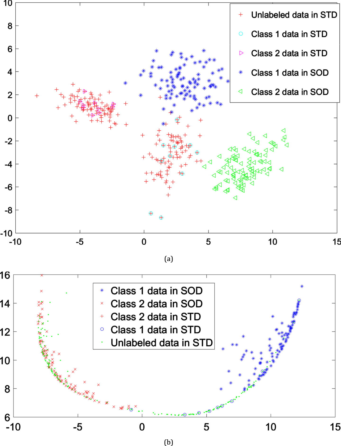
(a) An exemplary 2-dimensional data containing two classes in SOD (each class in SOD contains 100 data points) and also containing 200 data points in STD (where only 10 percent of data points in STD are labeled, i.e., 10 data points per each class in STD are labeled). It is worthy of being mentioned that 180 data points (90 data points per class) in STD are unlabeled. While the SVM classifier has a 92.62% accuracy rate on the original data, it has a 94.71% accuracy rate in the mapped data. The x-axis and y-axis stand for two features of dataset.

To do our experiment, we apply the proposed algorithm presented in Fig. 2 to the data points of our toy dataset depicted in Fig. 3a. After obtaining the kernel matrix of data points, the data points are transformed into their two leading components. Figure 3b is dedicated to the representation of the produced data points. Each class of data points in the original dataset depicted by Fig. 3a is transferred into the corresponding class of data points in the new dataset depicted by Fig. 3b. The support vector machine (SVM) classifier trained on the training data in Fig. 3a has a 92.62% accuracy rate on the testing data in Fig. 3a. The reported accuracy results in Fig. 3 are averaged over 30 independent runs. The SVM classifier with the same configuration trained on the training data in Fig. 3b has a 94.71% accuracy rate on the testing data in Fig. 3b.

4 Experimental study

We perform some empirical experiments to assess the efficacy of the proposed SemiSupervised SA approach. In the first subsection, some real datasets from the UCI repository [2] are chosen to be our benchmark. We evaluate a large number of the methods among the state of the art ones, and then compare their results to those of the proposed SemiSupervised SA approach.

In the second experimental study, we employ Land Mine datasets [16] as the benchmark. Again, we employ many of the methods among the state of the art ones as our baseline methods. Also, we use paired t-test for validation of the assessments. The third subsection of this section deals with a more popular dataset, i.e., Office+Caltech dataset, as the benchmark for assessing the proposed SemiSupervised SA approach against many of the methods among the state of the art ones. We consider different training and testing subsets from the Office+Caltech dataset here. In all cases, SVM is selected as our learner, and the Gaussian kernels are employed as its kernel function. The parameters of different methods have been set to their recommended values by their corresponding papers. The platform used for experimentations is MATLAB 2017a 64bit on a CorI7 CPU on a windows 7. During all experimentations, the platform is fix.

4.1 First experimental study

In the first experimental study, we employ the Breast-Cancer-Wisconsin dataset, Mushroom dataset, Liver dataset, and SA-Heart dataset (all are selected from the UCI machine learning repository) as our benchmark. The details of these datasets can be found in Table 2.

Table 2
Details of the used datasets in the first experimental study

Dataset name Class number Feature number Data point number

Breast-Cancer-Wisconsin dataset 2 9 699

Mushroom dataset 2 21 8124

Liver dataset 2 6 345

SA-Heart dataset 2 9 462

Dataset name	Class number	Feature number	Data point number
Breast-Cancer-Wisconsin dataset	2	9	699
Mushroom dataset	2	21	8124
Liver dataset	2	6	345
SA-Heart dataset	2	9	462

There are two types of space adjustment approaches used as baseline methods in this paper: (a) unsupervised ones, including TCA [1], Unsupervised Visual Domain Adaptation using Subspace Alignment (UVDASA) [19], KLIEP [6], Geodesic Flow Kernel (GFK) [20], Domain-Dependent Regularization (DDR) [31], Deep Learning by Interpolating between Domains (DLID) [29], Deep Domain Confusion (DDC) [30], Minimization of Inside-Cluster and Between Close Pairs of Samples Distances (MICBCPSD) [35], and (b) semi-supervised ones, including Cross Domain Support Vector Machine (CDSVM) [14] and Adaptive Support Vector Machine (ASVM) [15]. Note that unsupervised space adjustment approaches are different from clustering tasks [50].

To transform a single traditional standard dataset into a dataset suitable for SA, it is needed to be partitioned into two subsets: (I) data points in SOD and (II) data points in STD. For accomplishing the mentioned task, we employ the mechanism presented by Dai et al. [7]. It means, for the Mushroom dataset, data points are partitioned into two subsets according to its binary nominal feature named stalk-shape. The first subset, which includes data points with the attribute stalk-shape equal to value “e” (indicating enlarging in the dataset), is considered to contain data points in SOD. The other subset, which includes data points with the attribute stalk-shape equal to value “t” (indicating tapering in the dataset), is considered to contain data points in STD. It is also worthy of being mentioned that we omit the attribute stalk-root from the dataset because the attribute stalk-root contains missing values. With the same approach, the data points in SOD and the data points in STD are chosen from the SA-Heart dataset according to its binary nominal feature named Famhist.

For the Liver dataset, data points are partitioned into two subsets according to its continuous real-value feature named mean-corpuscular-volume. The first subset, which includes the data points that have a value equal to or less than $M_{mean - corpuscular - volume}$ in their attribute mean-corpuscular-volume, is considered to contain data points in SOD; and the other subset, which includes the data points that have a value greater than $M_{mean - corpuscular - volume}$ in their attribute mean-corpuscular-volume, is considered to contain data points in STD. The value $M_{mean - corpuscular - volume}$ is the median of the attribute mean-corpuscular-volume. With the same approach, the data points in SOD and the data points in STD are determined for the Breast-Cancer-Wisconsin dataset according to its continuous real-value feature named Mitoses.

We report any result in this subsection as an average on 30 independent runs. It means that each method is independently run 30 times on a given dataset. This results in a set of 30 independent results (or efficacies). The result of each independent run is also obtained through ten-fold cross-validation. Finally, its averaged result in those 30 runs is reported as the method efficacy on the given dataset.

Comparing the state of the art unsupervised SA and semi-supervised SA methods in terms of accuracy on (a) SA-Heart, (b) Liver, (c) Mushroom, and (d) Breast-Cancer-Wisconsin datasets can be observed in Fig. 4. The ratio of the data points in STD that belong to training data (and we use their labels during SA mechanism and classifier training) is variable and belongs to {0, 10, 20, 30, 40, 50}. The Non - SA method in Fig. 4 indicates the traditional machine learning method without applying any SA mechanism. It means the SVM classifier is trained on the training data, i.e., any data point with a label.

Fig. 4

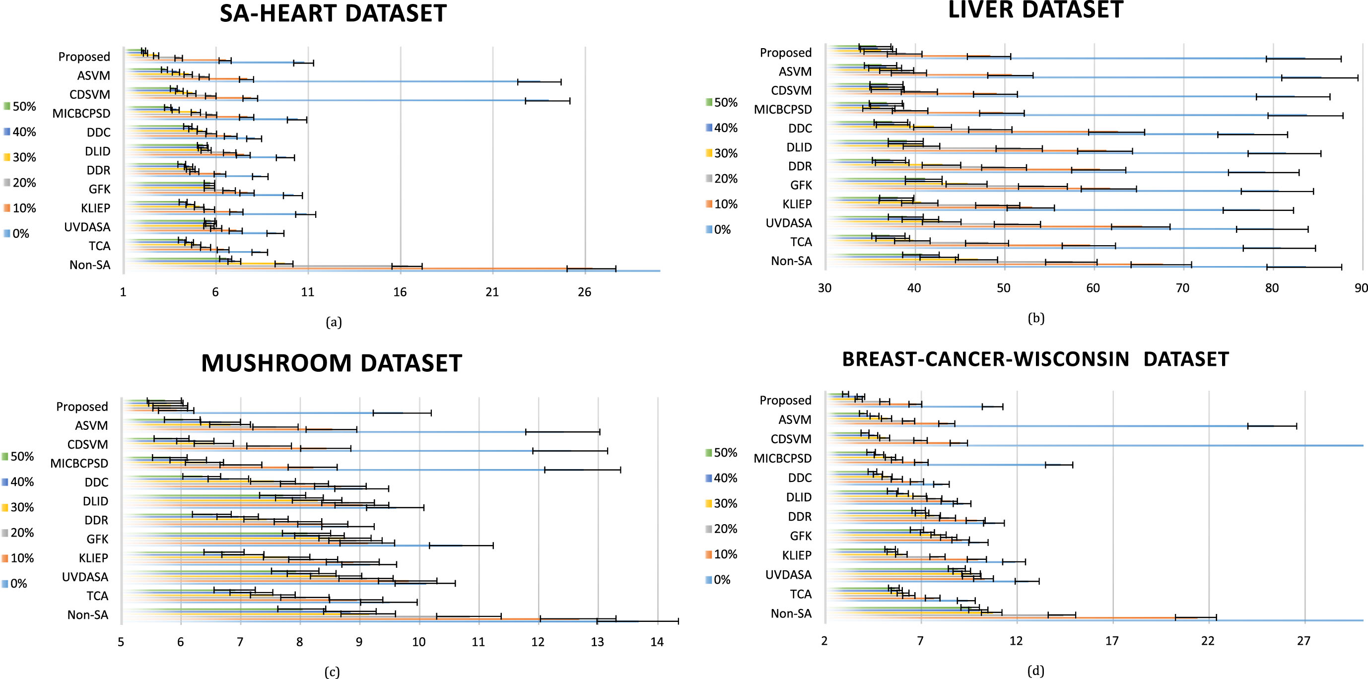
Comparing the state of the art unsupervised SA and semi-supervised SA methods in terms of accuracy on (a) SA-Heart, (b) Liver, (c) Mushroom, and (d) Breast-Cancer-Wisconsin datasets.

The results presented in Fig. 4 indicate that the Non - SA is the worst method due to its lack of any SA mechanism. It is significantly weak when there is 0% of training data points in STD (when all data points in SOD are used as our training dataset and all data points in STD are used as our testing dataset). Among the unsupervised approaches, the MICBCPSD method is the best. Among all approaches, the ASVM, CDSVM, and MICBCPSD approaches are the best ones. By adding more data points from data points in STD to training data points, the results of all methods get better. It means irrespective of the method, the greater the ratio of LSTD size to STD size, the better the performance. It can seem a clear statement for the semi-supervised SA methods. But, for the unsupervised SA methods, it is true because we need labels not only in performing the SA mechanism but also we need them in the training of the final SVM classifier.

4.2 Second experimental study

One of the most popular benchmarks, widely used in SA, can be the Land Mine collection of datasets [16], any of which contains two classes and nine features. There are many datasets in the Land Mine benchmark. The datasets numbered 1-10 and those numbered 20-24, i.e., 15 datasets, are the only datasets in the Land Mine benchmark that are used in the experiments of this subsection. The datasets numbered 1-10 have the same distribution. The other 5 datasets, i.e. the datasets numbered 20-24, are from different distributions. It means that the data points in our Land Mine benchmark come from 6 different distributions (data points of the datasets numbered 1-10, those of the dataset numbered 20, those of the dataset numbered 21, those of the dataset numbered 22, those of the dataset numbered 23, and those of the dataset numbered 24). We define seven datasets as follows: D1 (data points of the datasets numbered 1-5), D2 (data points of the datasets numbered 6-10), D3 (data points of the dataset numbered 20), D4 (data points of the dataset numbered 21), D5 (data points of the dataset numbered 22), D6 (data points of the dataset numbered 23), D7 (data points of the dataset numbered 24). In all experiments, the dataset D1 (or a subset of it) is used as the test dataset; it means that all of the test data points belong to D1. Therefore, D1 is the STD. In six experiments, respectively, one of our other six datasets, i.e., D2, D3, D4, D5, D6, and D7, is considered to be SOD.

The state of the art methods used in the previous subsection, in addition to Actively Transfer Domain Knowledge (ATDK) [16], are all used as baseline methods in this subsection. The ATDK method is considered to be a semi-supervised SA approach.

The results of the state of the art semi-supervised and unsupervised SA approaches in comparison with the proposed approach on different datasets of the Land Mine benchmark in terms of classification error are depicted in Fig. 5. The ratio of the size LSTD to the size STD (note that we use the labels of data points in LSTD during both SA mechanism and classifier training) is thirty percent. All of the results presented in Fig. 5 are averaged over 30 independent runs. The result of each independent run is also obtained through ten-fold cross-validation. Considering the results, we can find out that:

Fig. 5

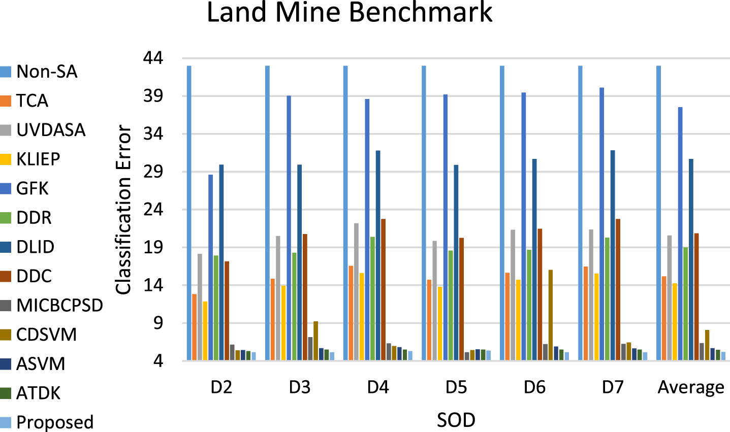
Efficacy comparison of the state of the art semi-supervised and unsupervised SA approaches with the proposed approach on different datasets of Land Mine benchmark in terms of classification error.

(a) the worst method is Non - SA due to its lack of any SA mechanism,

(b) the semi-supervised SA methods are better than the unsupervised SA ones because they use the labels of data points in LSTD,

(c) all of the SA methods perform better when they are trained on D2 because the data points in D2 and the ones in D1 are extracted from two similar distributions, and finally,

(d) the proposed method outperforms the other unsupervised SA methods in all cases and the other semi-supervised SA methods in most cases.

The summarized comparison of the state of the art semi-supervised and unsupervised SA approaches with the proposed approach on the Land Me benchmark validated by a two-sample t-test is presented in Table 3. Apparently, the proposed method is superior to the state of the art methods.

Table 3

The summarized results presented in Fig. 5 in terms of a two-sample t-test on 30 independent runs (with a 95% confidence value). Symbol “+” indicates the superiority of the proposed method to the corresponding method, symbol “–” indicates the superiority of the corresponding method to the proposed method, and symbol “±” indicates the proposed method is neither better nor weaker than the corresponding method validated by a two-sample t-test (with 95% confidence value)

Original Data Set	Non-SO	TCA	UVDASA	KLIEP	GFK	DDR	DLID	DDC	MICBCPSD	CDSVM	ASVM	ATDK
D2	+	+	+	+	+	+	+	+	+	±	±	±
D3	+	+	+	+	+	+	+	+	+	+	+	+
D4	+	+	+	+	+	+	+	+	+	+	+	±
D5	+	+	+	+	+	+	+	+	-	±	±	±
D6	+	+	+	+	+	+	+	+	+	+	+	+
D7	+	+	+	+	+	+	+	+	+	+	+	+
Average	6-0-0	6-0-0	6-0-0	6-0-0	6-0-0	6-0-0	6-0-0	6-0-0	5-0-1	4-2-0	4-2-0	3-3-0

The averaged times consumed for building the model (training phase) by different methods are presented in Fig. 6. As it is depicted, the execution time for the training phase of the proposed method is comparable to the most recent methods.

Fig. 6

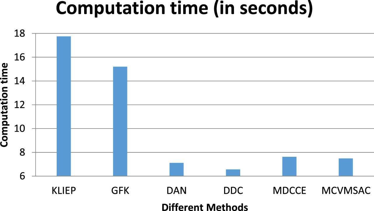
The execution time (in seconds) of the most recent methods averaged on 100 runs when D2 is considered to be SOD.

4.3 Third experimental study

The final experimental study is on an image dataset with four spaces: (a) dataset D1: the images taken by webcam, (b) dataset D2: the images collected from the amazon website, (c) dataset D3: the images taken by a digital camera, and (d) dataset D4: an auxiliary dataset of some images. The mentioned dataset is named Office+Caltech Benchmark (OCB) [3]. We depict two examples of Keyboard class (and two examples of Bag class) from different spaces in OCB in Fig. 7. All datasets D1, D2, D3, and D4 use images from a set of 10 shared classes. We employ the SURF attributes [33] and use a codebook of size equal to 800 [3, 20].

Fig. 7

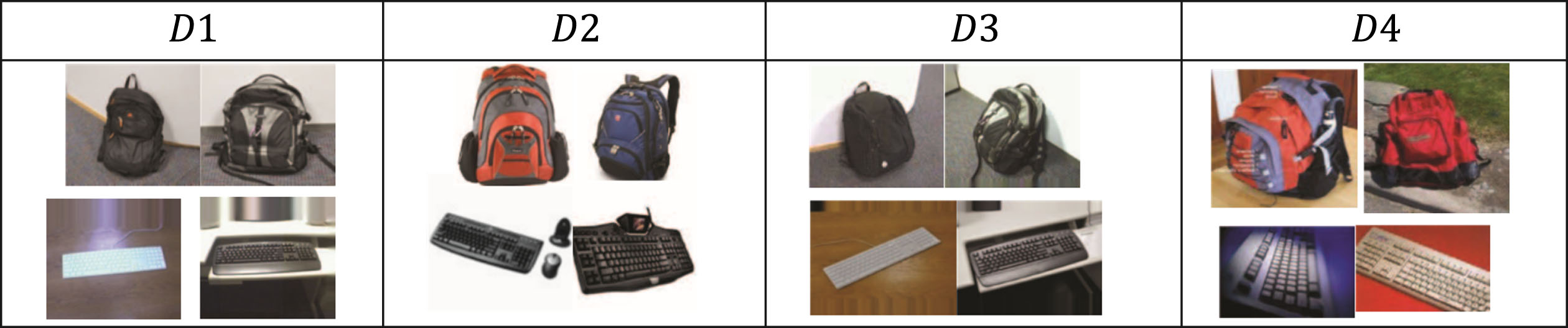
Two examples of Keyboard class (and two examples of Bag class) from different spaces in Office+Caltech Dataset [3].

We compare the efficacies of the state of the art SA algorithms with those of the proposed method on different configurations of the image dataset named OCB in terms of classification error in Fig. 8. The AsymML and SymML stand respectively for asymmetric and symmetric metric learning [3] as two semi-supervised SA approaches. The SGF stands for sampling geodesic flow as an unsupervised SA approach [20]. The SSSGF stands for the semi-supervised version of the SGF approach. The symbol “D1 -- > D3“ stands for the configuration in which D1 is SOD and D3 is STD. The ratio of the size LSTD to the size STD (note that we use the labels of data points in LSTD during both of SA mechanism and classifier training) is equal to five percent (at least one sample of each class from STD is added to the labeled data or the training dataset). The proposed SA method is superior to the state of the art SA methods irrespective of the pair (SOD, STD). GFK (and TCA to some extent) is overshadowed by the other methods because of their lack of supervision.

Fig. 8

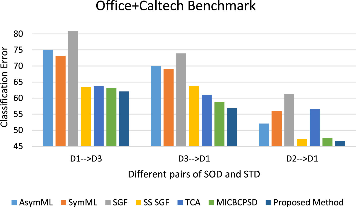
Comparing efficacies of the state of the art SA algorithms with efficacies of the proposed method on the image dataset named OCB.

In a broader study, we expand the results presented in Fig. 8 into some other SA methods and in more versatile pairs of (SOD, STD) configurations, and we depict them in Fig. 9. The ratio of the size LSTD to the size STD (note that we use the labels of data points in LSTD during both of SA mechanism and classifier training) is equal to thirty percent. The proposed SA method is superior to the state of the art SA methods irrespective of the pair (SOD, STD). The results presented in Table 4 sum up the results presented in Fig. 9.

Table 4

Summary of the results presented by Fig. 9. The symbol “+” indicates the superiority of the proposed method to the corresponding method, the symbol “-” indicates the superiority of the corresponding method to the proposed method, and the symbol “±” indicates the proposed method is neither better nor weaker than the corresponding method validated by a two-sample t-test (with a 95% confidence value)

	D4–>D2	D3–>D2	D1–>D2	D1–>D4	D2–>D3	D4–>D3	D1–>D3	D2–>D1	D4–>D1	D3–>D1	D2–>D4	D3–>D4
Non-SA	+	+	+	+	+	+	+	+	+	+	+	+	12-0-0
ASVM	+	+	+	+	+	+	+	+	+	+	+	+	12-0-0
CDSVM	+	+	+	-	+	+	+	+	+	+	±	+	10-1-1
ATDK	+	+	+	+	+	+	+	+	+	+	-	+	11-0-1
TCA	+	+	+	+	+	+	+	+	+	+	+	+	12-0-0
KLIEP	+	+	+	+	+	+	+	+	+	+	+	+	12-0-0
UVDASA	+	+	+	±	-	+	±	±	±	-	±	±	4-6-2
GFK	+	+	+	+	+	+	+	+	+	+	±	+	11-1-0
DLID	+	+	+	+	+	+	+	+	+	+	+	+	12-0-0
DDC	+	+	+	+	+	+	+	+	+	+	+	+	12-0-0
DDR	+	+	+	+	+	+	+	+	+	+	+	+	12-0-0
MICBCPSD	+	+	±	±	+	+	+	±	+	+	+	+	9-3-0
	12-0-0	12-0-0	11-1-0	9-2-1	11-0-1	12-0-0	11-1-0	10-2-0	11-1-0	11-0-1	8-3-1	11-1-0

Fig. 9

Broader experiments of Fig. 8 when the ratio of the size LSTD to the size STD is equal to thirty percent.

According to the results presented in Table 4, validated ba statistical test, the proposed method outperforms the state of the art methods aside from UVDASA. It still performs better than UVDASA marginally.

5 Conclusions and guideline for future works

We propose a kernelized semi-supervised space adjustment for data classification in this article. Our semi-supervised SA framework learns under three assumptions: (I) it is assumed that all data points in the SOD are labeled, and only a minority of data points in the STD are labeled, (II) the size of labeled samples in STD is very small comparing to the size of SOD, and (III) it is also assumed that the data samples in SOD and the data samples in STD have different distributions. The paper’s aim is to map the data from SOD a STD into an ShS. The proposed method does the mentioned mapping in such a way that structures of the data points before and after mapping are the same. The proposed method performs the mapping by a principal component analysis transformation on kernelized data. In the proposed method, it is tried to find a mapping that (a) can maintain the neighbors of data points after the mapping and (b) can take advantage of the class labels that are known in STD during transformation. Transforming our non-linear objective function into a semidefinite programming (SDP) problem, the paper proposes to solve the problem using an SDP solver. The examinations indicate the superiority of the learners trained on the data mapped by the proposed approach to the learners trained on the data mapped by the state of the art methods.

Compliance with ethical standards

Conflict of interest

The authors declare that they have no conflict of interest.

Ethical approval

This article does not contain any studies with human participants or animals performed by any of the authors.

Availability data and material

The datasets and materials can be accessed upon reader request.

Competing interests

Authors declare that there are no competing interests.

Funding

The authors declare there are no competing financial interests. The authors declare there are no financial supports.

Authors’ contributions

MA designed the study; MA wrote and edited the manuscript with help from other authors. MA generated all figures and tables. All authors have read and approved of the final version of the paper.

Footnotes

Acknowledgments

We want to thank all the reviewers.

References

Pan

S.J.

, Tsang

, Kwok

and Yang

, Domain adaptation via transfer component analysis, IEEE Transactions on Neural Networks 22 (2011), 199–210.

Bache

and Lichman

, UCI machine learning repository (2013). Available at https://archive.ics.uci.edu/ml

Saenko

, Kulis

, Fritz

and Darrell

, Adapting visual category models to new domains, in European Conference on Computer vision, 2010, pp, 213–226.

Pan

S.J.

and Yang

, A survey on transfer learning, IEEE Transactions on Knowledge and Data Engineering 22 (2010), 1345–1359.

Beijbom

, Domain adaptation for computer vision applications, Tech. Rep., University of California, San Diego, 2012.

Sugiyama

, Nakajima

, Kashima

, von Bünau

and Kawanabe

, Direct Importance Estimation with Model Selection and Its Application to Covariate Shift Adaptation, in Proceedings of Neural Information Processing Systems, 2007, pp. 1962–1965.

Dai

, Yang

, Xue

G.R.

and Yu

, Boosting for transfer learning, in International Conference on Machine Learning 2007, pp. 193–200.

Wan

, Pan

and Li

, Bi-weighting domain adaptation for cross-language text classification, in International joint conference on Artificial Intelligence, 2011, pp. 1535–1540.

Gopalan

, Li

and Chellappa

, Domain adaptation for object recognition: An unsupervised approach, in International Conference in Computer Vision, 2011, pp. 999–1006.

10.

Kulis

, Saenko

and Darrell

, What you saw is not what you get: Domain adaptation using asymmetric kernel transforms, in IEEE Conference on Computer Vision and Pattern Recognition, 2011, pp. 1785–1792.

11.

Jhuo

I.H.

, Liu

, Lee

D.T.

and Chang

S.F.

, Robust visual domain adaptation with low-rank reconstruction, in IEEE Conference on Computer Vision and Pattern Recognition, 2012, pp. 2168–2175.

12.

Chattopadhyay

, Krishnan

N.C.

and Panchanathan

, Topology Preserving Domain Adaptation for Addressing Subject Based Variability in SEMG Signal, in AAAI Spring Symposium: Computational Physiology, 2011, pp. 4–9.

13.

Howard

and Jebara

, Transformation Learning Via Kernel Alignment, in International Conference on Machine Learning and Applications, 2009, pp. 301–308.

14.

Jiang

, Zavesky

, fu Chang

and Loui

, Cross-domain learning methods for high-level visual concept classification, in International Conference on Image Processing, 2008, pp. 161–164.

15.

Yang

, Yan

and Hauptmann

A.G.

, Cross-domain video concept detection using adaptive SVMs, in International conference on Multimedia, 2007, pp. 188–197.

16.

Shi

, Fan

and Ren

, Actively Transfer Domain Knowledge, in European Conference on Machine Learning 2008, pp. 342–357.

17.

Baktashmotlagh

, Harandi

, Lovell

and Salzmann

, Unsupervised Domain Adaptation by Domain Invariant Projection, in International Conference on Computer Vision, 2013, pp. 769–776.

18.

Duan

, Xu

, Tsang

I.W.

and Luo

, Visual event recognition in videos by learning from web data, IEEE Transactions on Pattern Analysis and Machine Intelligence 34 (2012), 1667–1680.

19.

Fernando

, Habrard

, Sebban

and Tuytelaars

, Unsupervised Visual Domain Adaptation Using Subspace Alignment, in International Conference in Computer Vision, 2013, pp. 2960–2967.

20.

Gong

, Shi

, Sha

and Grauman

, Geodesic flow kernel for unsupervised domain adaptation, in IEEE Conference on Computer Vision and Pattern Recognition, 2012, pp. 2066–2073.

21.

Samanta

and Das

, Domain Adaptation Based on Eigen-Analysis and Clustering, for Object Categorization, in International Conference on Computer Analysis of Images and Patterns, LNCS, 2013, pp. 245–253.

22.

Hoffmann

, Kernel PCA for Novelty Detection, Pattern Recognition, 2007, pp. 863–874.

23.

Pezeshki

, Scharf

L.L.

and Chong

E.K.

, The geometry of linearly and quadratically constrained optimization problems for signal processing and communications, Journal of the Franklin Institute 347 (2010), 818–835.

24.

Boyd

and Vandenberghe

, Convex Optimization, Cambridge University Press, New York, NY, USA, 2006.

25.

Absil

P.A.

, Mahony

and Sepulchre

, Optimization Algorithms on Matrix Manifolds, Princeton University Press, 2008.

26.

Tagare

H.D.

, Notes on optimization on Stiefel manifolds, Tech. Rep., Department of Diagnostic Radiology, Department of Biomedical Engineering, Yale University, 2011.

27.

Wen

and Yin

, A feasible method for optimization with orthogonality constraints, Math Program 142 (2013), 397–434.

28.

Löfberg

, YALMIP: A Toolbox for Modeling and Optimization in MATLAB, in Proceedings of the CACSD Conference, Taiwan Taipei, 2004.

29.

Chopra

, Balakrishnan

and Gopalan

, Dlid: Deep learning for domain adaptation by interpolating between domains, In ICML Workshop on Challenges in Representation Learning, 2013.

30.

Tzeng

, Hoffman

, Zhang

, Saenko

and Darrell

, Deep domain confusion: Maximizing for domain invariance, CoRR, abs/1412.3474, 2014.

31.

Long

and Wang

, Learning transferable features with deep adaptation networks, CoRR, abs/1502.02791, 2015.

32.

Duan

, Xu

and Tsang

I.W.H.

, Domain adaptation from multiple sources: A domain-dependent regularization approach, IEEE Transaction Neural Network Learning System 23 (2012), 504–518. Available at https://vc.sce.ntu.edu.sg/transfer-learning-domainadaptation/domainadaptation-home.html

33.

Bay

, Ess

, Tuytelaars

and Gool

L.V.

, Speeded-up robust features (SURF), Computer Vision Image Understanding 110 (2008), 346–359.

34.

Oneto

, Bisio

, Cambria

and Anguita

, Semi-supervised Learning for Affective Common-Sense Reasoning, Cognitive Computation 9(1) (2017), 18–42.

35.

Pirbonyeh

, Rezaie

, Parvin

, Nejatian

and Mehrabi

, A linear unsupervised transfer learning by preservation of cluster-and-neighborhood data organization, Pattern Analysis and Applications (2018). doi.org/10.1007/s10044-018-0753-9.

36.

Caruana

, Multitask learning, Machine Learning 28(1) (1997), 41–75.

37.

Dai

, Yang

, Xue

and Yu

, Boosting for transfer learning, In Proceedings of the 24th International Conference on Machine Learning 2007, 193–200.

38.

Huang

, Smola

, Gretton

, Borgwardt

K.M.

and Scholkopf

, Correcting sample selection bias by unlabeled data, In Proceedings of the 19th Annual Conference on Neural Information Processing Systems, 2007.

39.

Sugiyama

, Nakajima

, Kashima

, Buenau

P.V.

and Kawanabe

, Direct importance estimation with model selection and its application to covariate shift adaptation, In Proceedings of the 20th Annual Conference on Neural Information Processing Systems, 2008.

40.

Ando

R.K.

and Zhang

, A framework for learning predictive structures from multiple tasks and unlabeled data, Journal of Machine Learning Research 6 (2005), 1817–1853.

41.

Argyriou

, Evgeniou

and Pontil

, Multitask feature learning, In Proceedings of the 19th Annual Conference on Neural Information Processing Systems, 2007, 41–48.

42.

Blitzer

, McDonald

and Pereira

, Domain adaptation with structural correspondence learning, In Proceedings of the Conference on Empirical Methods in Natural Language, 2006, 120–128.

43.

Raina

, Battle

, Lee

, Packer

and Ng

A.Y.

, Self-taught learning: Transfer learning from unlabeled data, In Proceedings of the 24th International Conference on Machine Learning 2007, 759–766.

44.

Daume

, III, Frustratingly easy domain adaptation, In Proceedings of ACL, pages 256–263, Prague, Czech Republic, 2007.

45.

Blitzer

, Dredze

and Pereira

, Biographies, bollywood, boom-boxes and blenders: Domain adaptation for sentiment classification, In Proceedings of ACL, pages 432–439, Prague, Czech Republic, 2007.

46.

Pan

S.J.

, Kwok

J.T.

and Yang

, Transfer Learning via Dimensionality Reduction, In Proceedings of the Twenty-Third AAAI Conference on Artificial Intelligence, 2008, 677–682.

47.

Zhu

, Ghahramani

and Lafferty

J.D.

, Semisupervised learning using gaussian fields and harmonic functions, In Proceeding of The 22th International Conference on Machine Learning 2003, 912–919.

48.

Bickel

, et al., Discriminative Learning Under Covariate Shift, Journal of Machine Learning Research 10 (2009), 2137–2155.

49.

Saeed

, Nam

, Ul-Haq

M.I.

and Bhatti

D.M.S.

, A Survey on Multidimensional Scaling, ACM Comput Surv 51(3) Article 47, 25 pages, 2018. https://doi.org/10.1145/3178155

50.

Almagbile

, Estimation of crowd density from UAVs images based on corner detection procedures and clustering analysis[J], Geo-spatial Information Science 22(1) (2019), 23–34.

51.

Liu

, Singleton

and Arribas-Bel

, A principal component analysis (PCA)-based framework for automated variable selection in geodemographic classification[J], Geo-spatial Information Science 22(4) (2019), 251–264.

52.

Cheng

, Yang

, Yao

, Guo

and Han

, When Deep Learning Meets Metric Learning: Remote Sensing Image Scene Classification via Learning Discriminative CNNs, IEEE Trans Geosci Remote Sens 56(5) (2018), 2811–2821.

53.

Pan

, Liu

, Guo

and Li

, Topic network: topic model with deep learning for image classification, J Electronic Imaging 27(03) (2018), 033009.

54.

Bhattarai

, Yadav

R.K.

, Gang

H.-S.

and Pyun

J.-Y.

, Geomagnetic Field Based Indoor Landmark Classification Using Deep Learning, IEEE Access 7 (2019), 33943–33956.

55.

Zheng

, Yang

, Zhang

and Zhang

, Improvement of Generalization Ability of Deep CNN via Implicit Regularization in Two-Stage Training Process, IEEE Access 6 (2018), 15844–15869.

56.

Zheng

, Tian

, Jiang

and Yang

, Layer-wise learning based stochastic gradient descent method for the optimization of deep convolutional neural network, J Intell Fuzzy Syst 37(4) (2019), 5641–5654.

A structure-protecting kernelized semi-supervised space adjustment for classification

Abstract

Keywords

1 Introduction

3 Problem statement and proposed solution

4.1 First experimental study

Table 2 Details of the used datasets in the first experimental study Dataset name Class number Feature number Data point number Breast-Cancer-Wisconsin dataset 2 9 699 Mushroom dataset 2 21 8124 Liver dataset 2 6 345 SA-Heart dataset 2 9 462

Compliance with ethical standards

Conflict of interest

Ethical approval

Availability data and material

Competing interests

Funding

Authors’ contributions

Footnotes

Acknowledgments

References

Table 2
Details of the used datasets in the first experimental study

Dataset name Class number Feature number Data point number

Breast-Cancer-Wisconsin dataset 2 9 699

Mushroom dataset 2 21 8124

Liver dataset 2 6 345

SA-Heart dataset 2 9 462