Indoor air quality prediction using optimizers: A comparative study

Abstract

Indoor air pollution (IAP) has become a serious concern for developing countries around the world. As human beings spend most of their time indoors, pollution exposure causes a significant impact on their health and well-being. Long term exposure to particulate matter (PM) leads to the risk of chronic health issues such as respiratory disease, lung cancer, cardiovascular disease. In India, around 200 million people use fuel for cooking and heating needs; out of which 0.4% use biogas; 0.1% electricity; 1.5% lignite, coal or charcoal; 2.9% kerosene; 8.9% cow dung cake; 28.6% liquified petroleum gas and 49% use firewood. Almost 70% of the Indian population lives in rural areas, and 80% of those households rely on biomass fuels for routine needs. With 1.3 million deaths per year, poor air quality is the second largest killer in India. Forecasting of indoor air quality (IAQ) can guide building occupants to take prompt actions for ventilation and management on useful time. This paper proposes prediction of IAQ using Keras optimizers and compares their prediction performance. The model is trained using real-time data collected from a cafeteria in the Chandigarh city using IoT sensor network. The main contribution of this paper is to provide a comparative study on the implementation of seven Keras Optimizers for IAQ prediction. The results show that SGD optimizer outperforms other optimizers to ensure adequate and reliable predictions with mean square error = 0.19, mean absolute error = 0.34, root mean square error = 0.43, R² score = 0.999555, mean absolute percentage error = 1.21665%, and accuracy = 98.87%.

Keywords

Indoor air quality pollutants prediction system optimizers

1 Introduction

At an average, human beings, especially the elderly population and new-borns, spend almost 80–90% of their time in the indoor environments and hence are the most susceptible to indoor pollution [1]. Within the past few years, IAQ has become the main cause behind excessive exposure to harmful pollutants [2, 3].

Several studies conducted in the past 150 years show that non-industrial IAQ plays a major role in the decayed quality of public health [4]. Still, there is a lack of scientific interest related to IAQ research, monitoring and policy management in the developed countries. Currently, it is possible to improve IAQ by using the latest technological advancements [4]. Internet of Things (IoT) can be used to monitor IAQ in the building environment. It can be defined as a paradigm where different objects with sensing capabilities are connected to the internet [5, 6]. IoT is an effective approach to design flexible health care systems and also allows the development of real-time health monitoring platforms for efficient decision making [7]. IoT offers relevant requirements for IAQ monitoring using wearable sensors that can upload data to dedicated servers and smartphones for further analysis of measured parameters [8]. The IoT is also used for real-time transmission of collected physical information. Moreover, IoT can be further combined with artificial intelligence, machine learning and deep learning approaches to develop intelligent systems for IAQ management. These methods can help in Big Data analysis while supporting the development of reliable prediction systems for building health and general well-being.

Considering the impact of IAQ for occupational health, government and municipal authorities need to install real-time supervision systems to detect unhealthy situations for enhanced living environments, at least at highly populated public places such as hospitals and schools [9]. Usually, simple building air management steps taken by homeowners and building operators can lead to significant positive impacts on IAQ; preferably, they can avoid smoking indoors and switch to natural ventilation whenever required [10]. However, it is relevant to implement real-time supervision systems to detect unhealthy behaviour and to ensure adequate ventilation with proper use of heating, ventilation, and air conditioning (HVAC) systems.

IAQ monitoring and evaluation systems allow efficient monitoring and decision making to promote occupational health. Distributed as well as the local assessment of chemical concentrations (e.g., pollution monitoring and gas spill detection) is relevant for safety and security applications. It also contributes to enhanced control on HVAC systems for energy efficiency [11, 12]. IoT based IAQ measurement provides a consistent stream of data for informed decision-making and reliable management of building automation systems [13, 14]. Furthermore, the prediction models can help building occupants to take preventive steps for enhanced IAQ, especially for children, elderly and people that are already suffering from serious respiratory health issues [15].

This paper presents an experimental analysis of efficient IoT based IAQ monitoring system. Seven different optimizers are used to design prediction model and their performance is compared. The main contribution of this paper is to provide a comparative study regarding the performance of Keras optimizers for predicting IAQ to design a reliable system for enhanced public health and well-being. The main objective is to reduce the prediction error to take adequate decisions in order to prevent serious building health problems for enhanced occupational health. Also, if the hours of forecasting can be increased, the occupants can follow relevant preventive measures to stay safe ahead of time. The rest of the paper is divided into four different sections, where the first section provides a background of the study stating the relevance of PM on IAQ along with related work done by previous researchers in this domain. The second section describes information about the materials and methods used for the development of the prediction system. The third section provides a comparison between seven different optimizers for the IAQ prediction system, along with results and discussions. And the last section is dedicated to the conclusion of this experimental analysis.

1.1 Background

Poor IAQ is rising as a significant challenge that leaves a relevant impact on the poorest and unprotected individuals worldwide [10]. Its association with human well-being is comparable to sexually transmitted diseases and tobacco use [10, 16]. The Environmental Protection Agency (EPA) in the United States takes the responsibility to develop regulations for maintaining indoor and outdoor air quality. Studies published by EPA also reveal that indoor pollutant levels are approximately one hundred times higher than outdoor pollutant levels, leading to some of the most significant environmental problems affecting general well-being [17].

There is a wide range of primary and secondary pollutants that contribute to poor IAQ; however, PM levels are recognized as major contributing parameters for decayed public health [18]. For routine monitoring and regulatory purposes, ambient PM is divided into two different quantities: PM₁₀ and PM_2.5. They represent mass concentrations of tiny particles collected by automatic systems as per international sampling standards related to ‘inhalable’ and ‘respirable’ particles. M_10–2.5, particles with the aerodynamic diameter >2.5 microns, but≤nominal 10 microns are defined as coarse fraction particles. Particles with diameter <1 micron are represented by PM_1.0. Furthermore, “Ultrafine” particles (UFP) are the particles with diameter < 0.1 microns (100 nm) in size [18].

PM is a multifaceted combination of liquefied and solid biological and mineral particles suspended in the air [19, 20]. PM generally includes dirt, dust, smoke, soot, and liquid droplets that can penetrate the lower airways of humans leading to severe harmful health effects. Indoor exposure to PM in developing countries increases the risk of acute lower respiratory infections [21, 22]. Several studies reveal that excessive exposure to PM levels is closely associated with mortality among young children [23, 24]. At the same time, it is a prominent cause of several chronic health problems, including chronic obstructive pulmonary disease, cardiovascular disease, and lung cancer among adults [25, 26].

Approximately 60,000 premature deaths are reported every year in the United States, and they are directly linked to poor air quality levels. The cost of healthcare facilities for treating diseases associated with air quality reach $150 billion [27]. As per a report presented by the European Environment Agency in the year 2016, air pollution caused 400,000 premature deaths within the European Union (EU). PM levels lead to 412,000 premature deaths in 41 different European countries 374,000 were reported in the EU [28]. Moreover, the cost of dealing with the harmful effects of air pollutants emitted from industrial facilities in 2012 was estimated somewhere around 59 to 189 billion euros in the EU [29]. The highly populated cities in India contribute to the highest pollution levels in the world, and the capital city of Delhi is mentioned on the top of the list. As per a study conducted by CNN in the year 2019, 21 out of the world’s 30 most polluted cities were from India [30]. The statistics of the year 2016 reveal that 140 million people out of 1.38 billion population in are affected by air quality, which is ten times worst as compared to the safe limit set by WHO [31]. Poor IAQ is the second major cause behind the increased mortality rate in India [32]. The 2018 Environment Performance Index Results report ranked India 177th among 180 countries based on 24 performance indicators covering ecosystem vitality and environmental health [33]. Moreover, over 1,00,000 deaths are reported in 29 Indian cities due to rising PM2.5 levels [34]. The adverse effects of ultrafine air particles are further linked to lung health and systemic circulation, where toxic components can cause potential tissue damage and inflammation [35]. It is necessary to notice that PM exposure is ubiquitous, and there is no defined and studied “safe” level. Hence, behavioural modification strategies can play a considerable role in enhanced overall health and well-being. The technology inspired PM monitoring and prediction systems can help policymakers to develop solid strategies for maintaining public health. That is why several researchers in the past few years have contributed their ideas in this direction. Numerous experimental studies from recent years are highlighted in Section 1.2.

1.2 Related work

Ghaemi et al. [36] proposed a Spatio-temporal system designed using the LaSVM-based online algorithm for dynamic prediction of air pollution in Tehran. The authors used meteorological data on carbon monoxide (CO), nitrogen dioxide (NO₂), sulfur dioxide (SO₂), ozone (O₃), and PM₁₀ from few target locations in Tehran. These pollutant concentrations were further used to calculate Air Quality Index (AQI) and then a prediction system was designed to estimate those values based on past monitoring. This system was able to predict AQI values for the next 24 hours with a root mean square error (MSE) of 0.54, the overall accuracy of 0.71, and a coefficient of determination equal to 0.81.

Another air quality prediction system was proposed by Zheng et al. [37] with the Multiple Kernel Learning approach. The four parameters used in this experimental study were O₃, NO₂, SO₂, PM, fine suspended particulates and respirable suspended particulates. The performance of the proposed system was further compared with the Random Forest (RF), classical autoregressive integrated moving average (ARIMA) model, support vector machine (SVM), long short-term memory (LSTM) and multiple-layer perceptron (MLP) neural network.

Soh et al. [38] designed an adaptive deep learning model for predicting air quality using spatial-temporal relations. This model was developed based on two datasets collected from 76 different locations of 23 cities of Taiwan and Beijing. The prediction system was mainly designed for predicting PM_2.5 based on wind direction, wind speed, temperature, humidity, PM_2.5, and PM₁₀ features. The system was able to forecast air quality for 48 hours using a combination of different neural networks, including LMST, Convolution Neural Network (CNN), and Artificial Neural Network (ANN) for extracting spatial-temporal relations.

Zhu et al. [39] proposed an air quality forecasting system using machine learning methods that could provide a prediction for around 24 hours. This study focused on three air pollutants: SO₂, PM_2.5 and O₃. The data was collected from two different weather stations located in the two suburban residential areas of Illinois. The authors in this study presented refined models for predicting IAQ by using advanced regularization techniques for performance optimization.

Tiwari et al. [40] also designed an air pollution level prediction system by considering four major pollutant concentrations: O₃, CO₂, SO₂, and NO₂. The authors of this study presented a feed-forward ANN-based model for predicting IAQ. The three input parameters applied at the input of ANN were Mean, 1^st Hourly Max and 1^st Max Value, whereas the output parameter was AQI. Furthermore, the ARIMA model was used to validate the predicted AQI.

In this experimental analysis, we designed an IoT based monitoring system for measuring essential IAQ parameters, and the prediction system was further developed using Keras optimizers. Although there are several libraries and frameworks available for handling time series analysis, the authors decided to work with Keras due to its ability to handle small datasets more efficiently. This open-source library is also preferred for the simplicity of coding environment, core architecture, and ability to run on the top of relevant frameworks such as TensorFlow, Theano, and R. The details about data collection, pre-processing and system development are described in the further sections.

2 Data collection and pre-processing

2.1 Dataset

Chandigarh is a union territory in India and is the capital of two neighbouring states, Punjab and Haryana. The estimated population of the city is 1.06 million with a higher number of vehicles and industrial units that lead to severe air pollution. This experimental analysis is carried out to estimate the state of IAP by measuring pollutant concentrations in the area that is badly affected by poor air quality. The sensor network was installed in the cafeteria of an educational institute (National Institute of Technical Teacher’s Training and Research) in Chandigarh city. The cafeteria stays populated throughout the day with peak traffic between 11:00 am to 11:30 am and 4:00 pm to 4:30 pm. The sensor network was placed close to the cooking area. The data was recorded for 6 months, two readings per hour, from 5th April to 4th September 2019.

As per WHO, the pollution index for Chandigarh city is 51.32. Moreover, air quality and air pollution are moderate, with an estimated value of 54.57 and 45.43, respectively. The PM10 level usually stays around 110, whereas PM2.5 is observed to be 59. However, the PM10 pollution level in the city is reported to be very high around the year. On the other side, the temperature typically varies between 48- and 106-degrees Fahrenheit over the year, and humidity stays within the estimated range of 24% to 97%. But as the vehicle traffic and industrial pollution is increasing with each passing day, the scenario may be more complicated in the coming years [41]. Hence, an early evaluation of air pollution levels and their impact is necessary.

2.2 Requirements:

Hardware requirements:

Arduino Uno

ESP8266 Module

SDS011 PM Sensor

DHT11 Sensor

Connecting wires

Software requirements:

Arduino IDE

Python

NumPy library

Seaborn library

Keras optimizer library

2.3 Methodology

The design of the prediction system is based on the real-time data collected using IoT sensor networks installed in Chandigarh City. The framework of the methodology is given in Fig. 1.

Fig. 1

Framework of the methodology.

The entire process can be categorized into three stages as data collection, data pre-processing and prediction model design. The detailed explanation of the methodology is given below.

2.3.1 Hardware design and data collection:

For analysing the levels of IAP and to design a prediction system for timely indication of critical instances, an IoT sensor network with PM, temperature, and humidity sensor was developed. Real-time data was collected with the help of the Arduino Uno based sensor network that uses the SDS011 sensor for measuring PM_2.5, PM₁₀ and DHT11 for measuring temperature and humidity. Table 1 shows the specifications of the essential hardware used for the cyber-physical system. The data was sent to the ThingSpeak channel for online storage by using the ESP8266 module. The diagram representing a sensor network for measuring pollutant concentrations is shown in Fig. 2.

Table 1
Specifications of sensors used for designing an IAQ monitoring system

Hardware Parameters Measuring rate Accuracy Power consumption info

SDS011 PM2.5, PM10 0.0–999.9μg/m3 15% and±10μg/m3 Voltage: 5 V Current: 70 mA±10 mA

DHT11 Temperature and Relative Humidity Temperature: 0–50°C Temperature: ±2°C Voltage: 3–5.5 V

Humidity: 20–90% Humidity: ±5% RH Operating current: 0.3 mA (measuring) 60 uA (standby)

Hardware	Parameters	Measuring rate	Accuracy	Power consumption info
SDS011	PM2.5, PM10	0.0–999.9μg/m3	15% and±10μg/m3	Voltage: 5 V Current: 70 mA±10 mA
DHT11	Temperature and Relative Humidity	Temperature: 0–50°C	Temperature: ±2°C	Voltage: 3–5.5 V
		Humidity: 20–90%	Humidity: ±5% RH	Operating current: 0.3 mA (measuring) 60 uA (standby)

Fig. 2

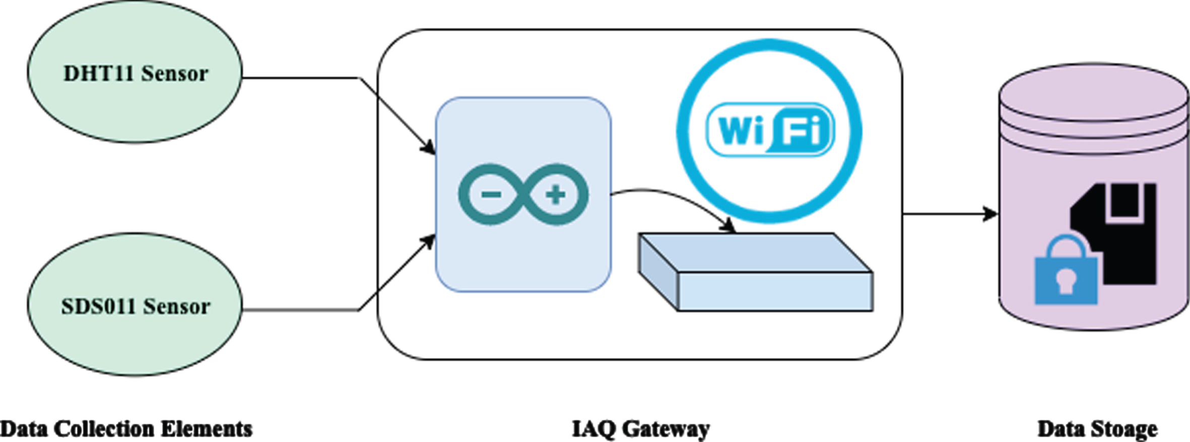
Framework of IoT sensor network for measuring pollutant concentration.

Table 1 shows the specifications of data collection elements used to record real-time measurements from the target monitoring area. However, the accuracy of the sensors installed is a crucial factor to verify the reliability of the monitoring system.

Reliability tests for sensors: DHT11 sensor was considered for this study due to its finest temperature and humidity measurement range with the accuracy between 2 to 5%. This sensor comes in pre-calibrated form from the industry. However, in order to ensure accuracy in measurements, the performance was compared with the standard temperature and humidity measurement meter (Honeywell TM005X) available in the lab.

The decision for selection of SDS011 laser sensor over other low-cost sensors was supported by existing studies conducted by early researchers [42 –44]. PM NOVA sensor was also pre-calibrated in the factory; however, the reliability test is required to ensure its accuracy for the IAQ monitoring system. The reliability test was conducted after 24 hours of a pre-heating period that is required to ensure accurate readings in a particular environment. The reliability of the sensor was continuously tested against the monitoring air station operated and maintained by the pollution control board in the city. The performance of the sensor was stable and within the accuracy range specified by the manufacturers. In order to maintain the accuracy of readings, careful sensor placement procedures were followed so that the normal flow of air cannot be blocked towards the chamber of the laser dust sensor.

Specifications of IAQ Gateway: IAQ Gateway consists of Arduino Uno and ESP8266 Wi-Fi module. ESP8266 is a self-contained system on chip with integrated TCP/IP protocol stack. It works on the basis of IEEE 802.11 standards and uses a Wi-Fi channel with 20 to 25 MHz band for communication. This module comes with a self-calibrated radio frequency (RF); hence, there is no need to add external RF parts for operation. The microcontroller uses AT commands over UART channels with a default baud rate of 115200 to communicate with the ESP8266 module.

The sensor network recorded data for four parameters PM_2.5, PM₁₀, temperature, and humidity. The natural deposition process of PM is greatly affected by relative humidity and temperature. Studies reveal that temperature has a negative correlation with PM₁₀, whereas relative humidity has a positive correlation with PM₁₀ [45].

The pollutant concentrations are further used to determine the AQI. It is basically an indicator of pollution levels as defined by EPA in the United States for public use. The formula specified for AQI calculations is given by Equation 1. $I = \frac{I_{high} - I_{low}}{C_{high} - C_{low}} (C - C_{low}) + I_{low}$ (1)

Where I represent AQI, C is pollutant concentration, C_lowC_low is a concentration breakpoint, which is equal to or less than C. C_highC_high is a concentration breakpoint that is equal to or greater than C. I_lowI_low and I_highI_high are the index breakpoints corresponding to C_lowC_low and C_highC_high, respectively. By using this equation, the AQI for real-time IAQ data of IoT sensor network located in Chandigarh city is calculated. This data was further pre-processed and trained with the help of optimizers. The details are described in the further sections.

2.3.2 Data pre-processing

The collected air pollution data and calculated AQI values are paired together to create the desired data format that can be further processed through the prediction model. The hourly mean values of the recorded parameters were processed. However, the recorded data had several missing values and multiple records at some hours during 6 months of monitoring. To deal with the missing values and inappropriate entries in the dataset, the dataset was pre-processed. Masking approach was used to impute the missing values in the dataset, and the rows having NaN values were dropped to clean the data. After data pre-processing, a dataset containing relevant values of parameters was obtained. For visualization of available multidimensional data Kernel Density Estimation (KDE) algorithm is utilized. It helps to plot the shape of distribution by keeping the density of the observations in one axis and height along the other axis. The matrix plot of the pairwise relationship between parameters (AQI, PM10, PM2.5, Temperature and Humidity) of the available training dataset is shown in Fig. 3.

Fig. 3

Pairwise relationship between AQI, PM10, PM2.5, Temp and Hum parameters of the available training dataset.

2.3.3 Feature analysis and normalization:

In order to design a prediction system, first of all, it is essential to define input features for the network. For the proposed system, the prediction label was assigned to AQI, and rest four parameters (Temp, Hum, PM10, and PM2.5) were considered as input features. Descriptive statistics of these features were obtained to get more insights into the shape of each attribute. The model generated several statistical values for each attribute in the input training data: mean, std, min, max, 25%, 50% and 75%; where mean represents mean of each input parameter, std represents Bessel-corrected sample standard deviation, min and max show minimum and maximum values in the distribution, respectively. The 25%, 50% and 75% are sample quantile values. In general, quantiles are the points in the distribution with respect to the rank order of the values present in the distribution. In this, 25% shows lower quartile, 75% is the upper quartile and 50% is middle quantile that can be also referred to as median. The list of extracted descriptive statistics for each attribute are shown in Table 2.

Table 2
Statistical properties of four input parameters under consideration.

Parameter Mean Std Min 25% 50% 75% Max

Temperature 31.61 1.593 28.3 30.5 31.4 32.7 35.2

Humidity 68.08 7.214 34.0 65.0 70.0 73.0 85.0

PM2.5 19.42 9.892 2.1 13.0 17.2 24.5 52.5

PM10 50.83 32.988 4.0 30.9 46.6 59.8 205.7

Parameter	Mean	Std	Min	25%	50%	75%	Max
Temperature	31.61	1.593	28.3	30.5	31.4	32.7	35.2
Humidity	68.08	7.214	34.0	65.0	70.0	73.0	85.0
PM2.5	19.42	9.892	2.1	13.0	17.2	24.5	52.5
PM10	50.83	32.988	4.0	30.9	46.6	59.8	205.7

After feature extraction, the entire input dataset was converted into a float datatype by scaling all values between 0 and 1; this task is performed by using Equation 2. The scaling is performed because optimize-based prediction model works best when the input values fall in the range of 0 and 1. $Norm Data = \frac{x - mean (x)}{std (x)}$ (2)

Where Norm Data represent normalized dataset, x is the parameter value, mean (x) represent mean of respective parameter value and std (x) represent the standard deviation of the respective parameter value. The dataset was further divided into three parts: 60% for training, 20% for testing and 20% for validation of the model.

2.4 Optimizers

In this section, the authors describe the different approaches for IAQ prediction. The selection of the right optimizer and configuration of a set of parameters can help to squeeze even the last bit of accuracy for the prediction model. This experimental analysis is based on seven different optimizers, and their performance is compared based on mean absolute error (MAE), MSE, Root Mean Square Error (RMSE), R² Score (Co-efficient of determination), Mean Absolute Percentage Error (MAPE) and Accuracy. In the section, the optimizers tested by the authors are succinctly explained.

Stochastic Gradient Descent:

Gradient descent (GD) is a fundamental technique for training and optimizing intelligent systems. It basically considers the following equation for minimizing loss function and for enhancing system accuracy: $θ = θ - η \cdot \nabla J (θ) θ = θ - η \cdot \nabla J (θ)$ (3)

Where ‘η’ represents learning rate, ‘∇J (θ)’ is the gradient of loss function-J(θ) w.r.t parameters- ‘θ.’

Stochastic Gradient Descent (SGD) optimizer is known as the simplest form of GD in terms of its behaviour and concept as well [46]. It starts with a small learning rate and follows the gradient on the cost surface. After each iteration, it generates new weights that are better than the old ones obtained in the previous iterations. It mainly includes support for learning rate decay and momentum. In the training network, a random batch of samples is taken for each iteration and values of θ are updated every time.

The mathematical representation for SGD is shown below: $θ = θ - η \cdot \nabla J (θ; x^{(i)}; y^{(i)})$ (4)

Where, x⁽ⁱ⁾ and y⁽ⁱ⁾ indicate training examples.

Adagrad:

Adagrad or Adaptive Learning Rate optimizer simply follows the learning rate (η) to adapt as per the input parameters [47]. It works by making small updates for the frequent parameters and big updates for the infrequent parameters. Hence, this optimizer is widely recommended for handling sparse data.

In the previous method, we made updates at once for all parameters θ because all θ_i components were having the same η . But in the case of Adagrad, all parameters θ_i follow different η at every time step t. For Adagrad, we set $g_{t, i} θ_{t + 1, i} = θ_{t, i} - \frac{η}{\sqrt{G_{t, ii} + ɛ}} . g_{t, i}$ as the gradient of the loss function with respect to θ_i at time step t. The equation is shown below: $θ_{t + 1, i} = θ_{t, i} - \frac{η}{\sqrt{\sum_{i = 1}^{t} g_{i}^{2} + ɛ}} . g_{t, i}$ (5)

Where ∈ = 10e - 8.

The biggest benefit of Adagrad is that it does not require manual tuning of η. In most cases, the default value is taken as 0.01.

Adadelta:

Adadelta is basically an extension of Adagrad; it works for removing the decaying learning rate problem of the previous algorithm. Instead of using all previously squared gradients, Adadelta restricts the window of all accumulated past gradients to a fixed size w [48].

Instead of storing w previous squared gradients, Adadelta defines the sum of gradients in a recursive manner as the decaying mean of the past squared gradients. The final formula for Adadelta is defined below: $Δ θ_{t} = - \frac{η}{\sqrt{E {[g^{2}]}_{t} + ɛ}} . g_{t}$ (6)

Here the denominator just represents the Room Mean Square (RMS) error criterion of the gradient and can be written as RMS [g] _t ; hence, the 5th equation can be rewritten as: $Δ θ_{t} = - \frac{η}{RMS {[g]}_{t}} . g_{t}$ (7)

One important thing to note about Adadelta is that one need not put special efforts for setting η.

RMSprop:

Room Mean Squared Propagation (RMSprop) algorithm is also a kind of adaptive learning rate method [49]. Both Adadelta and RMSprop were developed independently in the same duration to resolve the radically diminishing learning rate problem of Adagrad. RMSprop is almost identical to the first update vector of Adadelta and can be given as: ${Δ θ}_{t} = θ_{t} - \frac{η}{\sqrt{E {[g^{2}]}_{t} + ɛ}} . g_{t}$ (8)

Note that RMSprop also divides the model learning rate by the exponentially decaying average of squared gradients.

Adam:

Adaptive Moment Estimation (Adam) optimizer is recommended for average [50]. This algorithm makes use of adaptive learning rates for each parameter and momentum to ensure fast convergence. While storing the exponentially decaying average of the past squared gradients such as AdaDelta, Adam also keeps track of the exponentially decaying average of the past gradients m(t). The final formula for updating parameter with Adam optimizer is: $θ_{t + 1} = θ_{t} - \frac{η}{\sqrt{{\hat{v}}_{t}} + ɛ} . {\hat{m}}_{t}$ (9)

Here v_t and m_t are the uncentered variance and mean of the gradients, respectively.

This optimizer works well in the practical environment with its fast convergence rate and comparatively higher learning speed.

Adamax:

The v_t factor of the Adam optimizer update rule leads to the inversely proportional scaling of the gradient with respect to the ℓ₂ norm of the past gradients as well as the current gradient |g_t|²

Here, the basic equation is represented as: $v_{t} = β_{2}^{p} v_{t - 1} + (1 - β_{2}^{p}) {| g_{t} |}^{p} v_{t}$ (10)

It was further updated by Kigma and Ba [51], to achieve more stable value. In order to avoid confusion with Adam, the new equation was represented by u_t that represents infinity norm-constrained v_t. The new equation can be shown as: $u_{t} = β_{2}^{\infty} v_{t - 1} + (1 - β_{2}^{\infty}) {| g_{t} |}^{\infty}$ (11)

Where β₂ represents decay rate whose default value is 0.999. With this improvement in the equation, the final Adamax update rule can be represented as: $θ_{t + 1} = θ_{t} - \frac{η}{u_{t}} . {\hat{m}}_{t} θ_{t + 1} = θ_{t} - \frac{η}{u_{t}} . {\hat{m}}_{t}$ (12)

It is important to mention that u_t is dependent on the max operation; it does not go towards zero as v_t and ${\hat{m}}_{t}$ in Adam. Hence, there is no need to calculate bias correction for u_t.

Nadam:

Generally, Adam is represented as the combination of momentum and RMSprop; on the other side, the Nadam optimizer or Nesterov-Accelerated Adaptive Moment Estimation is the combination of Adam and Nesterov Accelerated Gradient (NAG) [52]. Hence, the final update rule for Nadam can be represented by adding the Nesterov Momentum term to the Adam equation. The new rule can be shown as: $θ_{t + 1} = θ_{t} - \frac{η}{\sqrt{{\hat{v}}_{t}} + ɛ} . (β_{1} {\hat{m}}_{t} + \frac{(1 - β_{1}) g_{t}}{1 - β_{1}^{t}})$ (13)

Where β₁ is the decay rate with a default value of 0.9.

All these optimizer algorithms present small parametric variations over one another that add the difference to their overall performance in designing prediction system for IAQ.

2.5 Prediction model

Following the concept of seven different optimizers discussed in section 2.4, the IAQ prediction model was designed. The main idea was to compare the performance of all these optimizers based on relevant regression metrics so that the most efficient optimizer can be identified to design a real-time, intelligent IAQ monitoring and prediction system. Figure 4 shows the stages of the IAQ prediction model designed for this comparative study. The data obtained from the hardware module is fed to the prediction algorithm. However, instead of putting raw data as it is, the pre-processing stage is added to the system. The first most step at this stage was to clean the dataset by following the masking approach discussed in section 2.3.2. After that, the response label was applied to the AQI parameter and the rest parameters (PM10, PM2.5, Temp and Hum) were considered as input features to train the prediction model. It is crucial to mention at this stage that statistical feature extraction was used to describe the dataset. None of the input parameters were discarded at this stage since several studies report that PM concentrations are greatly affected by temperature and humidity levels [35 , 53]. Hence, all four input parameters were used for training to ensure that their overall impact is utilized for designing efficient prediction model. After feature selection and label assignment, the data were normalized by following the technique mentioned in section 2.3.3. The normalized data was then used to train model containing seven different optimizers and then their performance was compared using six different regression metrics, including MSE, MAE, RMSE, R² score, MAPE and Accuracy. Based on these metrics, the best model was selected for designing an intelligent IAQ prediction system that can be used for real-time analysis in the future. The results obtained after training the prediction model with the seven optimizers are discussed in the next section.

Fig. 4

Stages of IAQ prediction model for comparing performance of seven optimizers.

3 Results and discussions

This section describes the results obtained with each optimizer and their performance comparisons. After obtaining a normalized dataset, the sequential model for prediction system was initialized with 64 nodes in the hidden layer. Rectified Linear Unit (ReLU) was applied as an activation function for all seven optimizers. The major rationale for using ReLU is that it allows gradient to be non-zero and ensure automatic recovery during the training process. It involves simple and fast mathematical computations as compared to Sigmoid and Tanh activation functions; hence, is believed to be computationally less expensive.

The training set was applied to all seven optimizers separately, and model performance was evaluated in terms of MSE, MAE, RMSE, R² Score, MAPE and Accuracy. At the initial level, 1000 epochs were set for all seven optimizers and then early stopping condition was applied with a common patience parameter value of 10. Early stopping condition allows the training to stop when chosen performance measures stop making further improvements. It helps to avoid unnecessary computations for the optimization model and describe how fast it can converge for the best performance.

For all optimizers, the learning rate was adjusted to reduce the error and, ultimately, to obtain the best possible prediction for AQI with that particular optimizer. The prediction performance of optimizers was finally compared on the basis of important regression metrices. A comparison of the obtained parameter values is shown in Table 3.

Table 3
Comparison table showing performance of prediction models with seven different optimizers

Optimizer Learning Rate Patience Parameter Best Epoch MSE MAE RMSE R² Score MAPE Accuracy

SGD 0.001 10 50 0.19 0.34 0.43 0.999555 1.126650 98.87 %

Adagrad 0.02 10 140 0.20 0.35 0.45 0.999343 1.326938 98.67 %

Adadelta 0.03 10 600 0.21 0.36 0.46 0.999488 1.176639 98.82 %

RMSprop 0.001 10 50 0.24 0.38 0.48 0.999417 1.449454 98.55 %

Adam 0.001 10 80 0.30 0.41 0.55 0.999342 1.456049 98.54 %

Adamax 0.001 10 100 0.21 0.34 0.45 0.999515 1.173592 98.83 %

Nadam 0.002 10 80 0.25 0.37 0.5 0.999437 1.227379 98.77 %

Optimizer	Learning Rate	Patience Parameter	Best Epoch	MSE	MAE	RMSE	R² Score	MAPE	Accuracy
SGD	0.001	10	50	0.19	0.34	0.43	0.999555	1.126650	98.87 %
Adagrad	0.02	10	140	0.20	0.35	0.45	0.999343	1.326938	98.67 %
Adadelta	0.03	10	600	0.21	0.36	0.46	0.999488	1.176639	98.82 %
RMSprop	0.001	10	50	0.24	0.38	0.48	0.999417	1.449454	98.55 %
Adam	0.001	10	80	0.30	0.41	0.55	0.999342	1.456049	98.54 %
Adamax	0.001	10	100	0.21	0.34	0.45	0.999515	1.173592	98.83 %
Nadam	0.002	10	80	0.25	0.37	0.5	0.999437	1.227379	98.77 %

From the comparison table, it is clearly visible that the best performance for AQI prediction was presented by the SGD optimizer with MSE = 0.19 AQI and MAE = 0.34 AQI, RMSE = 0.43, R² Score = 0.99955, and MAPE = 1.12665. Furthermore, the accuracy of model trained with SGD optimizer was highest (98.87%) as compared to model trained with other six optimizers. The above performance was obtained with the low learning rate of 0.001, and it was recorded at a very early stage during the 50th epoch. Very close performance was shown by Adagrad with MSE = 0.20, MAE = 0.35, RMSE = 0.45 and Adamax with MSE = 0.21, MAE = 0.34, RMSE = 0.45 respectively. However, in terms of the overall accuracy, Adamax performed comparatively better with the accuracy value of 98.83%; however, it was restricted to 98.67% in case of Adagrad. Adagrad was able to achieve this performance with the learning rate of 0.02; whereas Adamax managed to achieve this performance with the learning rate the same as SGD, i.e., 0.001. However, the epoch for both these optimizers was comparatively high with count 140 for Adagrad and 100 for Adamax. Adadelta also performed well to reduce error but it took 600 epochs to achieve this performance and that too with a higher learning rate value of 0.03. Nevertheless, in terms of the accuracy measure, it stood third with 98.82%. Although RMSprop and Adam converged faster but the error reduction as well as the overall accuracy was poor as compared to SGD.

The graphical plot for MSE and MAE of SGD is shown in Fig. 5, and graphical representation of these performance metrics for other 6 optimizer models are shown in Fig. 6. and 7. One can observe minute variation in the graphs but even a slight improvement in accuracy is valuable for the AQI prediction model as it can prevent severe health issues in the building environment.

Fig. 5

Graphical plot of SGD performance metrics a) MAE and b) MSE.

Fig. 6

Comparative graphical representation of MSE for six models.

Comparison in terms of RMSE, R² Score, MAPE and Accuracy are shown in Fig. 8. RMSE is the most widely used metrics for evaluation of regression models; its value is desired to be low as prediction models with larger errors are not reliable. As sesen from Table 3 and Fig. 8, SGD shows the least RMSE value as compared to other models. R² Score is generally defined as the ratio between the MSE of the model and MSE of the baseline where MSE (model): Mean Squared Error of the predictions against the actual values MSE (baseline): Mean Squared Error of mean prediction against the actual values. The value usually varies between -∞ to 1. Higher the value (close to 1), better the model. In the given model, the highest R² Score is reported for the SGD model with 0.999555. MAPE is another commonly used measure to determine forecasting accuracy due to its advantage of interpretability and scale-independency. As it is a measure of error, the ideal value is desired to be at the lower side of the scale. For the given comparative study, SGD presents the minimum value of MAPE (1.126650) as compared to other optimizers. The accuracy measure is generally evaluated for classification problems. However, to compare the performance of different optimizers for designing a reliable prediction system, the forecasting accuracy of different optimizers was also determined using MAPE. The best results were presented by SGD with highest accuracy (98.87%).

Fig. 7

Comparative graphical representation of MAE for six models.

Fig. 8

Model performance comparison in terms of RMSE, R² Score, MAPE and Accuracy.

Generally, SGD follows frequent updates, and the parameters have a high variance. It leads to more fluctuation of the loss function to the different intensities. As a result, this algorithm works better to discover new; and moreover, better local minima, i.e. the smallest value of the function on the entire domain of the function. That is why SGD has shown better convergence with the least error for the AQI prediction. The error curve of SGD based prediction model is shown in Fig. 9. and it shows the Gaussian distribution.

Fig. 9

Error histogram of AQI prediction for SGD model.

Consequently, SGD is the best solution for designing an IAQ prediction system; the graph showing prediction accuracy with respect to the true values is shown in Fig. 10. It shows that prediction values are closely aligned to the true values. Therefore, the SGD optimizer can ensure reliable prediction results using real-time IAQ monitoring data.

Fig. 10

Predictions for AQI with respect to the true values of AQI.

Furthermore, the performance of the SGD based prediction model is compared with the existing literature. The comparison on the basis of a few essential parameters is performed in Table 4.

Table 4

Comparison of the SGD-based prediction model with existing literature

Authors	IAQ Parameters	Prediction Model	Predicted Parameters	Prediction Duration	Model Evaluation Parameters
Ghaemi et al. [36]	CO, NO2, SO2, O3, PM10	LaSVM	AQI	24 hours	RMSE = 0.54, Accuracy = 0.71, Coefficient of determination = 0.81
Zheng et al. [37]	O3, NO2, SO2, PM, fine suspended particulates and respirable suspended particulates	Multiple Kernel Learning	Air quality health index (AQHI) and PM2.5	1, 3, 6, 9, and 12 hours’	AQHI:
					1 h: MSE = 0.030
					3 h: MSE = 0.028
					6 h: MSE = 0.028
					9 h: MSE = 0.203
					12 h: MSE = 0.609
					PM2.5
					1 h: MSE = 0.806
					3 h: MSE = 0.945
					6 h: MSE = 1.275
					9 h: MSE = 1.133
					12 h: MSE = 1.536
Soh et al. [38]	Wind direction, wind speed, temperature, humidity, PM2.5, and PM10	Spatial-temporal relations	PM2.5	48 hours	RMSE = 5.25 –5.65
Zhu et al. [39]	SO2, PM2.5, O3	Multi-task learning	PM2.5, O3 and SO2	24 hours	RMSE: O3 –0.0845 –0.11535
					PM2.5 = 0.0368
					SO2 = 0.03248
Best model from Table 3	PM2.5, PM10, temperature and humidity	SGD optimizer	AQI	96 hours	MSE = 0.19
					MAE = 0.34
					RMSE = 0.43
					R² Score = 0.999555
					MAPE = 1.12665
					Accuracy = 98.87%

From the analysis of Table 4, it is clear that the SGD optimizer-based prediction model demonstrates prediction for 96 hours; whereas the range was limited to 24 hours [36, 39], 48 hours [38] and 12 hours [37] for the existing methods. At the same time, the MSE, MAE, RMSE, R² Score, MAPE and Accuracy value of the SGD based model for AQI prediction is far better than the existing systems.

4 Conclusion

In this paper, a comparative analysis for AQI prediction using optimizers was given. We evaluated these models with the help of real-time data collected from the IoT sensor network. The acquisition module was installed at a cafeteria of college campus in Chandigarh city for assessment of IAQ. The system was designed for two main IAQ parameters: PM₁₀ and PM_2.5; however, it is also applicable to other pollutants as well. The temperature and humidity parameters were also considered to assess thermal comfort along with IAQ. The sensors used for this model were calibrated using standard procedures and reliability tests were conducted so that higher accuracy can be ensured for training. The experimental design and comparative study show that the SGD optimizer can provide highly accurate predictions as compared to Adam, Adagrad, Adadelta, Nadam, RMSProp and Adamax optimizer. The SGD optimizer-based model have MSE and MAE of 0.19 and 0.34 respectively for a prediction of 96 hours. Furthermore, other evaluation metrics are also presented favorable results for SGD based model with RMSE = 0.43, R2 score = 0.999555, MAPE = 1.12665 and Accuracy = 98.87%. Based on the experiments, the following conclusions can be obtained: (1) The SGD optimizer-based prediction model offers better prediction ability as compared to other optimizers. (2) This system is capable of forecasting severe air pollution in a more efficient manner as compared to existing methods. (3) Feature extraction and learning rate adjustment perform a significant role in improved AQI forecasting.

The main limitations of this study are related to the experimental analysis, which is restricted to only two IAQ parameters (PM₁₀ and PM_2.5) and two thermal comfort parameters (temperature and humidity). Moreover, this study is limited to comparative analysis only; it is possible to add more value by designing an automated system with a standalone app that could predict real-time results for IAQ. As future work, we are planning to work on a higher number of pollutants by considering their relative impact on the health of building occupants. Furthermore, the quality of the model can be improved by using long-duration monitoring as it can provide more stable and adequate results for prediction. The authors want to use different machine learning methods to find the best model for enhanced system performance so that the system architecture can be improved. The proposed air quality prediction system will be automated to provide an open-source application programming interface (API) that can be easily used by everyone. This API should allow agile and easy manipulation of the prediction system with real-time data collected by third-party air quality monitoring systems. In order to assess the state of IAP, it is first important to know the parameters that affect IAQ and the level of exposure to the building occupants. This model provides insights into the monitoring and control mechanisms as it allows people to apply preventive measures ahead of time by observing predictions. Therefore, pollution studies, prevention policies and management techniques are greatly dependent on prediction system models.

References

The National Human Activity Pattern Survey (NHAPS): a resource for assessing exposure to environmental pollutants | Journal of Exposure Science & Environmental Epidemiology, https://www.nature.com/articles/7500165 (accessed May 03, 2020).

Walsh

P.J.

, Dudney

C.S.

and Copenhaver

E.D.

, Indoor air quality. CRC Press, (1983).

Marques

and Pitarma

, A Cost-Effective Air Quality Supervision Solution for Enhanced Living Environments through the Internet of Things, Electronics 8(2) (2019), 170. doi: 10.3390/electronics8020170

Sundell

, On the history of indoor air quality and health, Indoor Air 14(s7) (2004), 51–58. doi: 10.1111/j.1600-0668.2004.00273.x

Marques

, Garcia

and Pombo

, A Survey on IoT: Architectures, Elements, Applications, QoS, Platforms and Security Concepts, in C. X. Mavromoustakis, G. Mastorakis, and C. Dobre, Eds. Cham: Springer International Publishing 22 (2017), 115–130.

Marques

, Ambient Assisted Living and Internet of Things, in Harnessing the Internet of Everything (IoE) for Accelerated Innovation Opportunities, P.J.S. Cardoso, J. Monteiro, J. Semião and J.M. F. Rodrigues, Eds. Hershey, PA, USA: IGI Global, (2019), 100–115.

Marques

, Pitarma

, Garcia

N.M.

and Pombo

, Internet of Things Architectures, Technologies, Applications, Challenges, and Future Directions for Enhanced Living Environments and Healthcare Systems: A Review, Electronics 8(10) (2019), 1081. doi: 10.3390/electronics8101081

Gubbi

, Buyya

, Marusic

and Palaniswami

, Internet of Things (IoT): A vision, architectural elements, and future directions, Future Generation Computer Systems 29(7) (2013), 1645–1660. doi: 10.1016/j.future.2013.01.010

Marques

and Pitarma

, Monitoring and control of the indoor environment, in 2017 12th Iberian Conference on Information Systems and Technologies (CISTI), Lisbon, Portugal, Jun. (2017), 1–6. doi:10.23919/CISTI.2017.7975737

10.

Bruce

, Perez-Padilla

and Albalak

, Indoor air pollution in developing countries: a major environmental and public health challenge, Bulletin of the World Health Organization 78(9) (2000), 1078–1092.

11.

De Vito

, et al., Cooperative 3D Air Quality Assessment with Wireless Chemical Sensing Networks, Procedia Engineering 25 (2011), 84–87. doi: 10.1016/j.proeng.2011.12.021

12.

Marques

and Pitarma

, IAQ Evaluation Using an IoT CO2 Monitoring System for Enhanced Living Environments, in Á. Rocha, H. Adeli, L. P. Reis, and S. Costanzo, Eds. Cham: Springer International Publishing 746 (2018), 1169–1177.

13.

Preethichandra

D.M.G.

, Design of a smart indoor air quality monitoring wireless sensor network for assisted living, (2013), 1306–1310. doi:10.1109/I2MTC.2013.6555624

14.

Marques

and Pitarma

, An Internet of Things-Based Environmental Quality Management System to Supervise the Indoor Laboratory Conditions, Applied Sciences 9(3) (2019), 438. doi: 10.3390/app9030438

15.

Marques

and Pitarma

, Promoting Health and Well-Being Using Wearable and Smartphone Technologies for Ambient Assisted Living Through Internet of Things, inY. Farhaoui, Ed. Cham: Springer International Publishing 81 (2020), 12–22.

16.

Marques

and Pitarma

, An Indoor Monitoring System for Ambient Assisted Living Based on Internet of Things Architecture, International Journal of Environmental Research and Public Health 13(11) (2016), 1152. doi: 10.3390/ijerph13111152

17.

Seguel

J.M.

, Merrill

, Seguel

and Campagna

A.C.

, Indoor Air Quality, American Journal of Lifestyle Medicine 11(4) (2016), 284–2895.

18.

Heal

M.R.

, Kumar

and Harrison

R.M.

, Particles, air quality, policy and health, Chemical Society Reviews 41(19) (2012), 6606. doi: 10.1039/c2cs35076a

19.

Kampa

and Castanas

, Human health effects of air pollution, Environmental Pollution 151(2) (2008), 362–367. doi: 10.1016/j.envpol.2007.06.012

20.

Utell

M.J.

and Frampton

M.W.

, Acute Health Effects of Ambient Air Pollution: The Ultrafine Particle Hypothesis, Journal of Aerosol Medicine 13(4) (2000), 355–359. doi: 10.1089/jam.2000.13.355

21.

Gumede

P.R.

and Savage

M.J.

, Respiratory health effects associated with indoor particulate matter (PM2.5) in children residing near a landfill site in Durban, South Africa, Air Qual Atmos Health 10(7) (2017), 853–860. doi: 10.1007/s11869-017-0475-y

22.

Jerrett

, et al., Comparing the Health Effects of Ambient Particulate Matter Estimated Using Ground-Based versus Remote Sensing Exposure Estimates, Environmental Health Perspectives 125(4) (2017), 552–559. doi: 10.1289/EHP575

23.

Keet

C.A.

, Keller

J.P.

and Peng

R.D.

, Long-Term Coarse Particulate Matter Exposure Is Associated with Asthma among Children in Medicaid, Am J Respir Crit Care Med 197(6) (2018), 737–746. doi: 10.1164/rccm.201706-1267OC

24.

Isiugo

, et al., Indoor particulate matter and lung function in children, Science of The Total Environment 663 (2019), 408–417. doi: 10.1016/j.scitotenv.2019.01.309

25.

Salvi

, et al., Indoor Particulate Matter<2.5μm in Mean Aerodynamic Diameter and Carbon Monoxide Levels During the Burning of Mosquito Coils and Their Association With Respiratory Health, Chest 149(2) (2016), 459–466. doi: 10.1378/chest.14-2554

26.

Mukherjee

and Agrawal

, A Global Perspective of Fine Particulate Matter Pollution and Its Health Effects, in Reviews of Environmental Contamination and Toxicology Volume 244, 244 P. de Voogt, Ed. Cham: Springer International Publishing, (2017), 5–51.

27.

National Weather Service, “Why Air Quality Is Important,” Why Air Quality Is Important. https://www.weather.gov/safety/airquality (accessed Jul. 21, 2019).

28.

European Environment Agency, Air quality in Europe: 2019 report. (2019).

29.

Holland

, Spadaro

, Misra

and Pearson

, Costs of Air Pollution from European Industrial Facilities 2008–2012—An Updated Assessment, EEA Technical Report, (2014).

30.

“India has 21 of the world’s 30 cities with the worst air pollution - CNN.” https://edition.cnn.com/2020/02/25/health/most-polluted-cities-india-pakistan-intl-hnk/index.html (accessed May 07, 2020).

31.

“Dirty air: how India became the most polluted country on earth.” https://ig.ft.com/india-pollution (accessed May 07, 2020).

32.

Saini

, Dutta

and Marques

, A comprehensive review on indoor air quality monitoring systems for enhanced public health, Sustainable Environment Research 30(1) (2020), 6. doi: 10.1186/s42834-020-0047-y

33.

E.P. Index, Environmental performance index, Yale University and Columbia University: New Haven, CT, USA, (2018).

34.

The Economic Times, Over 1 lakh deaths in 29 cities due to air pollution: Study, Feb. 15, (2020). https://economictimes.indiatimes.com/news/politics-and-nation/over-1-lakh-deaths-in-29-cities-due-to-air-pollution-study/articleshow/74144139.cms (accessed May 07, 2020).

35.

Saini

, Dutta

and Marques

, Particulate Matter Assessment in Association with Temperature and Humidity: An Experimental Study on Residential Environment, in Proceedings of International Conference on IoT Inclusive Life (ICIIL 2019), NITTTR Chandigarh, India, Singapore, (2020), 167–174. doi:10.1007/978-981-15-3020-3_15

36.

“LaSVM-based big data learning system for dynamic prediction of air pollution in Tehran. - PubMed - NCBI.” https://www.ncbi.nlm.nih.gov/pubmed/29679160 (accessed Jan. 13, 2020).

37.

Zheng

, Li

, Lu

and Ruan

, A Multiple Kernel Learning Approach for Air Quality Prediction, Advances in Meteorology, 2018 (2018), 1–15. doi: 10.1155/2018/3506394

38.

Soh

P.-W.

, Chang

J.-W.

and Huang

J.-W.

, Adaptive Deep Learning-Based Air Quality Prediction Model Using the Most Relevant Spatial-Temporal Relations, IEEE Access 6 (2018), 38186–38199. doi: 10.1109/ACCESS.2018.2849820

39.

Zhu

, Cai

, Yang

and Zhou

, A Machine Learning Approach for Air Quality Prediction: Model Regularization and Optimization, BDCC 2(1) (2018), 5. doi: 10.3390/bdcc2010005

40.

Tiwari

, Upadhyay

, Singhal

, Garg

and Bisht

, Air Pollution Level Prediction System 8(6) (2019), 8.

41.

“Air quality in Chandigarh worsens as number of vehicles go up,” Hindustan Times, Sep. 13, (2018). https://www.hindustantimes.com/punjab/air-quality-in-chandigarh-worsens-as-number-of-vehicles-go-up/story-IStBEj6Bqlv261WK8nxpPI.html (accessed May 07, 2020).

42.

Liu

H.-Y.

, Schneider

, Haugen

and Vogt

, Performance Assessment of a Low-Cost PM2.5 Sensor for a near Four-Month Period in Oslo, Norway, Atmosphere 10(2) (2019), 41. doi: 10.3390/atmos10020041.

43.

, Jo

, Kim

and Han

, Development of an IoT-Based Indoor Air Quality Monitoring Platform, Journal of Sensors 2020 (2020), 1–14. doi: 10.1155/2020/8749764

44.

Badura

, Batog

, Drzeniecka-Osiadacz

and Modzel

, Evaluation of Low-Cost Sensors for Ambient PM _2.5 Monitoring, Journal of Sensors 2018 (2018), 1–16. doi: 10.1155/2018/5096540

45.

Hernandez

, Berry

T.-A.

, Wallis

and Poyner

, Temperature and humidity effects on particulate matter concentrations in a sub-tropical climate during winter., (2017). doi:10.7763/IPCBEE.2017.V102.10

46.

Bottou

, Large-Scale Machine Learning with Stochastic Gradient Descent, in Proceedings of COMPSTAT’2010, Y. Lechevallier and G. Saporta, Eds. Heidelberg: Physica-Verlag HD, (2010), 177–186.

47.

Ruder

, An overview of gradient descent optimization algorithms, arXiv preprint arXiv:1609.04747, (2016).

48.

Zeiler

M.D.

, ADADELTA: an adaptive learning rate method, arXiv preprint arXiv:1212.5701, (2012).

49.

Mukkamala

M.C.

and Hein

, Variants of rmsprop and adagrad with logarithmic regret bounds, in Proceedings of the 34th International Conference on Machine Learning-Volume 70, (2017), 2545–2553.

50.

, Yu

, Liu

and Kong

, A Recognition Method for Italian Alphabet Gestures Based on Convolutional Neural Network, in Intelligent Computing Theories and Application 11643, Huang

D.-S.

, Bevilacqua

, Premaratne,

, Eds. Cham: Springer International Publishing, (2019), 653–664.

51.

Kingma

D. P.

and Ba

, Adam: A method for stochastic optimization, arXiv preprint arXiv:1412.6980, (2014).

52.

Muliono

, Ham

and Darmawan

, Keystroke Dynamic Classification using Machine Learning for Password Authorization, Procedia Computer Science 135 (2018), 564–569.

53.

Fang

, et al., Relationship between fine particulate matter, weather condition and daily non-accidental mortality in Shanghai, China: A Bayesian approach, PLoS One 12(11) (2017), doi: 10.1371/journal.pone.0187933

Indoor air quality prediction using optimizers: A comparative study

Abstract

Keywords

1 Introduction

1.1 Background

1.2 Related work

2 Data collection and pre-processing

2.1 Dataset

2.2 Requirements:

2.3 Methodology

Table 2 Statistical properties of four input parameters under consideration. Parameter Mean Std Min 25% 50% 75% Max Temperature 31.61 1.593 28.3 30.5 31.4 32.7 35.2 Humidity 68.08 7.214 34.0 65.0 70.0 73.0 85.0 PM2.5 19.42 9.892 2.1 13.0 17.2 24.5 52.5 PM10 50.83 32.988 4.0 30.9 46.6 59.8 205.7

References