Uncertain production risk process with breakdowns and its shortage index and shortage time

1 Introduction

One type of production problems is about some continuous production cycles in which the data of cycle time and the production amount or cost are known. Muth [14] contributed to the first work of renewal process in production problems by taking the cycle times as random variables with exponential distribution functions and the production amounts as one unit each cycle, and then the work was extended by Papadopoulos [15] into the case in which the random distribution functions of the cycles times are non-identical. Furthermore, the model with multiple production lines was also solved by Papadopoulos [16]. However, in most practical production problem, it is unwise to assume that the machines used in production are continuously available and without any breakdowns. Therefore, Birge and Glazebrook [2] suggested a production model in which the cycle times are regarded as on-times plus off-times, that is, a production model with breakdowns. The breakdowns existing in the production model reduce the machine capacity, and the production amount may not be enough to satisfy the demand and then shortage occurs. Hence Groenevelt et al. [4] proposed safety level to handle the case with breakdowns where the crisp production rate and demand rate are known and the cycle times for demand are regarded as random variables. Moreover, for a production model with breakdowns and random demand, Parlar [17] applied random renewal reward theorem (Ross [18]) to calculating the average cost per time. Some applications of production process with breakdowns were proposed by Christer and Keddie [3] (block replacement policy) and Billatos and Kendall [1] (age replacement policy).

Probability theory is the best mathematical tool to deal with frequency. However, as one common type of emergency occurring in production, it is not easy to accurately forecast when the breakdowns happen. That means, the estimated distribution functions of the on-time and off-time (caused by breakdowns) in each cycle may not be closed enough to the frequency. Especially, for a new product, the data about the production amounts are inadequate and the practical distribution functions deviate far from the frequency. To make matters worse, even for an old product, the historical data about the cycle times and production amounts may become unavailable for estimating the distribution functions due to the unexpected breakdowns. In order to deal with the production model with breakdowns, Wang [19] regarded the cycle times as fuzzy random variables and applied fuzzy random renewal reward theorem (Zhao et al. [24]) to calculating the average cost per time. Following that, by separating back-order cost and holding cost from the production cost and regarding them as fuzzy random variables, a modified fuzzy random production model with breakdowns was introduced by Kumar and Goswami [5].

Unfortunately, in some practical production problems, neither probability theory nor fuzzy theory can be used to reasonably deal with the emergency such as breakdown (Liu [11]), and uncertainty theory proposed by Liu [7] and perfected by Liu [9] is the only suitable mathematical tool to measure the indeterminacy of breakdowns occurring in production. As an axiomatic mathematical branch, uncertainty theory was developed by a great number of scholars. In 2008, the concept of uncertain renewal process was introduced by Liu [8], and then in 2010 the concept of uncertain renewal reward process was presented by Liu [10]. Following that, by dividing the interarrival time into on-time and off-time, uncertain alternating renewal process was first suggested by Yao and Li [20]. Furthermore, uncertain delayed renewal process was proposed by Zhang et al. [23]. One important application of uncertain renewal process is the uncertain insurance model introduced by Liu [12] in 2013, which is essentially an uncertain process in which the interarrival times and claim amounts are assumed to be uncertain variables and the premium rate is crisp. After that, a theorem to evaluate the uncertainty distribution of ruin time of the uncertain insurance model was proved by Yao and Zhou [22], and a modified model was suggested by Yao and Qin [21] to solve the case in which both the claim process and premium process of the uncertain insurance model have to be considered as uncertain renewal reward processes.

For another important application, Lio and Liu [6] first proposed an uncertain production risk process and calculated its shortage index and shortage time. However, their model assumed that the production process has no any breakdown in every production cycle. This paper aims to modify the uncertain production risk process to evaluate the shortage index and shortage time with breakdowns. The rest of the paper is organized as follows: the modified uncertain production risk process with breakdowns is presented in Section 2. In Section 3, the concept of shortage index with breakdowns is proposed and some formulas are provided for its evaluation. In Section 4, the concept and the uncertainty distribution of shortage time with breakdowns are further given. Some numerical examples are documented in Section 5 and a concise conclusion is reviewed in Section 6.

2 Uncertain production risk process with breakdowns

In this section, an uncertain production risk process with breakdowns will be given based on the following notation:

Notation

ξ_1i: the i-th uncertain on-time, i = 1, 2, ⋯

ξ_2i: the i-th uncertain off-time, i = 1, 2, ⋯

ξ_1i + ξ_2i: the i-th uncertain cycle time, i = 1, 2, ⋯

N _t : the number of production cycle up to time t

η _i : the i-th uncertain production amouts, i = 1, 2, ⋯

P _t : total production amount up to time t

a: initial inventory level

b: demand rate The production problem we concern with is an uncertain production model with uncertain cycle times (i.e., the times consumed by one production cycle), uncertain production amounts and breakdowns. Due to the breakdowns existing in the production process, the uncertain cycle times should be divided into uncertain on-times and uncertain off-times. Let us suppose the uncertain on-times ξ₁₁, ξ₁₂, ⋯ are iid uncertain variables with a common uncertainty distribution Φ₁, and the uncertain off-times ξ₂₁, ξ₂₂, ⋯ are iid uncertain variables with a common uncertainty distribution Φ₂. By the operational law (Liu [10]), the uncertain cycle times ξ₁₁+ ξ₂₁, ξ₁₂ + ξ₂₂, ⋯ are iid uncertain variables with a common uncertainty distribution Φ ( y ) = sup x Φ 1 ( x ) ∧ Φ 2 ( y - x ) . Then the number of production cycles N _t up to time t is an uncertain renewal process. Essentially, the uncertain renewal process N _t is a maximal integer which makes n production cycles finish up to time t, i.e., N t = max n ≥ 0 { n | S n ≤ t }(1) where S₀ = 0 and S _n  = (ξ₁₁ + ξ₁₂) + (ξ₁₂ + ξ₂₂) + ⋯ + (ξ_1n + ξ_2n) for n ≥ 1. Moreover, an uncertain renewal process was proved by Liu [8] to have an uncertainty distribution G t ( x ) = 1 - Φ ( t ⌊ x ⌋ + 1 ) , ∀ x ≥ 0(2) where ⌊x⌋ is the maximal integer that is less than or equal to x. Now suppose the production amounts η₁, η₂, ⋯ are iid uncertain variables which have a common uncertainty distribution Ψ. Then the total production amount up to time t can be represented by an uncertain renewal reward process P t = ∑ i = 1 N t η i ,(3) and it was proved by Liu [10] to have an uncertainty distribution H t ( x ) = max k ≥ 0 ( 1 - Φ ( t k + 1 ) ) ∧ Ψ ( x k ) .(4) Here we assume Ψ (x/0) =1 for any x ≥ 0.

Given the fixed values for the initial inventory level a and demand rate b, the definition about the uncertain production risk process with breakdowns is presented as follows:

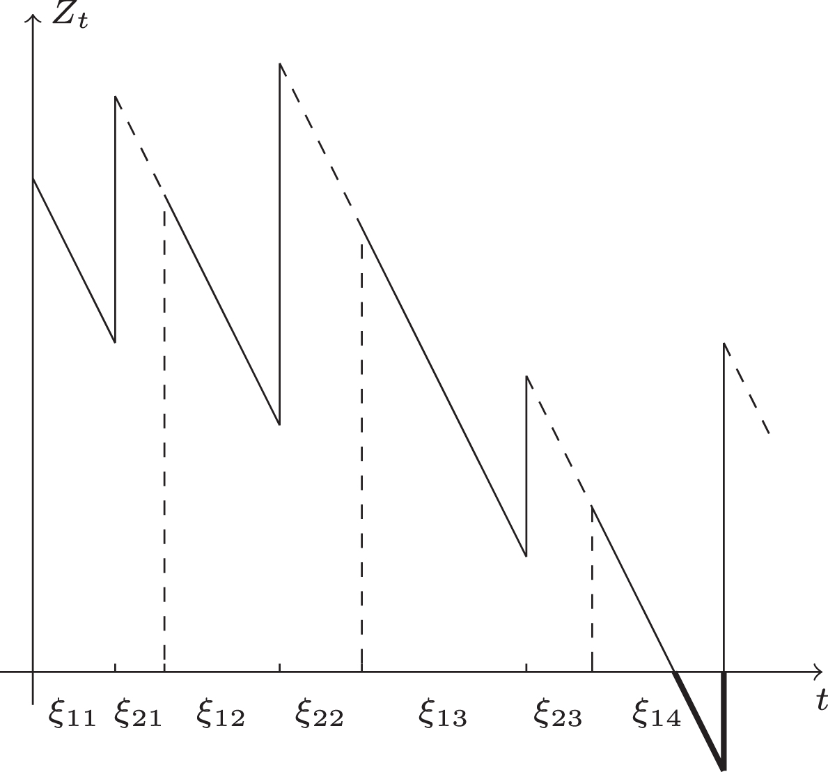
Definition 2.1. Let ξ₁₁, ξ₁₂, ⋯ be iid uncertain on-times, ξ₂₁, ξ₂₂, ⋯ be iid uncertain off-times, and η₁, η₂, ⋯ be iid uncertain production amounts. If a is the initial inventory level and b is the demand rate, then the uncertain production risk process with breakdowns is Z t = { a + ∑ i = 1 N t η i - bt , if ∑ i = 1 N t ( ξ 1 i + ξ 2 i ) ≤ t < ∑ i = 1 N t ( ξ 1 i + ξ 2 i ) + ξ 1 , N t + 1 a + ∑ i = 1 N t + 1 η i - bt , if ∑ i = 1 N t ( ξ 1 i + ξ 2 i ) + ξ 1 , N t + 1 ≤ t < ∑ i = 1 N t + 1 ( ξ 1 i + ξ 2 i )(5)

where N _t is the renewal process with uncertain cycle times ξ₁₁+ ξ₂₁, ξ₁₂ + ξ₂₂, ⋯

An example of the uncertain production risk process with breakdowns is revealed in Figure 1.

OPEN IN VIEWER

Fig.1

An Uncertain Production Risk Process with Breakdowns.

Shortage occurs when the quantity demanded is greater than the surplus inventory. Due to the breakdowns in the uncertain production risk process, the production capacity decreases or the production planning becomes unavailable. Hence the decision makers have to suffer shortage and solve the trouble caused by production risk. Lio and Liu [6] proposed the concept of shortage index to measure the belief degrees of shortage, but the shortage index was based on the case without breakdowns. Therefore, this section modifies the existing concept of shortage index and introduces the shortage index with breakdowns.

Shortage index with breakdowns is essentially the uncertain measure that the uncertain production risk process with breakdowns becomes negative.

Definition 3.1. Suppose Z _t is an uncertain production risk process with breakdowns. Then the shortage index with breakdowns is defined as Shortage = M { inf t ≥ 0 Z t < 0 } .(6)

Theorem 3.1. Suppose Z _t is an uncertain production risk process with breakdowns, a is the initial inventory level and b is the demand rate. Let ξ₁₁, ξ₁₂, ⋯ be iid uncertain on-times, ξ₂₁, ξ₂₂, ⋯ be iid uncertain off-times, and η₁, η₂, ⋯ be iid uncertain production amounts. If (ξ₁₁, ξ₁₂, ⋯), (ξ₂₁, ξ₂₂, ⋯) and (η₁, η₂, ⋯) are independent uncertain vectors, and those on-times, off-times and production amounts have continuous uncertainty distributions Φ₁, Φ₂ and Ψ, respectively, then the shortage index with breakdowns is Shortage = max k ≥ 1 sup y 1 , y 2 ≥ 0 ( 1 - Φ 1 ( y 1 k ) ) ∧ ( 1 - Φ 2 ( y 2 k - 1 ) ) ∧ Ψ ( b ( y 1 + y 2 ) - a k - 1 ) .(7) Here we set Φ 2 ( y 2 0 ) = { 0 , if y 2 < 0 1 , if y 2 ≥ 0 and Ψ ( b ( y 1 + y 2 ) - a 0 ) = { 0 , if b ( y 1 + y 2 ) - a < 0 1 , if b ( y 1 + y 2 ) - a ≥ 0 .

Proof. For each positive integer k, we define an uncertain process indexed by k as follows, Y k = a + ∑ i = 1 k - 1 η i - b ( ∑ i = 1 k ξ 1 i + ∑ i = 1 k - 1 ξ 2 i ) . Then Y _k is an independent increment process with an uncertainty distribution F k ( z ) = sup a + x - b ( y 1 + y 2 ) = z ( 1 - Φ 1 ( y 1 k ) ) ∧ ( 1 - Φ 2 ( y 2 k - 1 ) ) ∧ Ψ ( x k - 1 ) = sup y 1 , y 2 ≥ 0 ( 1 - Φ 1 ( y 1 k ) ) ∧ ( 1 - Φ 2 ( y 2 k - 1 ) ) ∧ Ψ ( z - a + b ( y 1 + y 2 ) k - 1 ) . It follows by extreme value theorem (Liu [12]) that for an independent increment process Y _k with uncertainty distribution F _k  (z), the minimum min k ≥ 1 Y k has an uncertainty distribution G ( z ) = max k ≥ 1 F k ( z ) . Since it is clear that Z _t eventually becomes negative if and only if Y _k  < 0 for some k, we get Shortage = M { inf t ≥ 0 Z t < 0 } = M { min k ≥ 1 Y k < 0 } = G ( 0 ) = max k ≥ 1 F k ( 0 ) . The theorem follows immediately.

Theorem 3.2. Suppose Z _t is an uncertain production risk process with breakdowns, a is the initial inventory level and b is the demand rate. Let ξ₁₁, ξ₁₂, ⋯ be iid uncertain on-times, ξ₂₁, ξ₂₂, ⋯ be iid uncertain off-times, and η₁, η₂, ⋯ be iid uncertain production amounts. If (ξ₁₁, ξ₁₂, ⋯), (ξ₂₁, ξ₂₂, ⋯) and (η₁, η₂, ⋯) are independent uncertain vectors, and those on-times, off-times and production amounts have regular uncertainty distributions Φ₁, Φ₂ and Ψ, respectively, then the shortage index with breakdowns is Shortage = max k ≥ 1 α k where α k = sup { α | a + ( k - 1 ) Ψ - 1 ( α ) - b ( k Φ 1 - 1 ( 1 - α ) + ( k - 1 ) Φ 2 - 1 ( 1 - α ) ≤ 0 }(8) for each k.

Proof. It follows from Theorem 3.1 that α k = sup y 1 , y 2 ≥ 0 ( 1 - Φ 1 ( y 1 k ) ) ∧ ( 1 - Φ 2 ( y 2 k - 1 ) ) ∧ Ψ ( b ( y 1 + y 2 ) - a k - 1 ) .(9) Therefore, for each k, the optimal solution ( y 1 k * , y 2 k * ) of the maximization problem (9) satisfies α k = ( 1 - Φ 1 ( y 1 k * k ) ) ∧ ( 1 - Φ 2 ( y 2 k * k - 1 ) ) = Ψ ( b ( y 1 k * + y 2 k * ) - a k - 1 ) . Now for each k, suppose ( y ˜ 1 k , y ˜ 2 k ) is a solution such that α k = 1 - Φ 1 ( y ˜ 1 k k ) = 1 - Φ 2 ( y ˜ 2 k k - 1 ) . Then we have 1 - Φ 1 ( y ˜ 1 k k ) ≤ 1 - Φ 1 ( y 1 k * k ) , 1 - Φ 2 ( y ˜ 2 k k - 1 ) ≤ 1 - Φ 2 ( y 2 k * k - 1 ) and then y ˜ 1 k ≥ y 1 k * , y ˜ 2 k ≥ y 2 k * . Hence we have Ψ ( b ( y ˜ 1 k + y ˜ 2 k ) - a k - 1 ) ≥ Ψ ( b ( y 1 k * + y 2 k * ) - a k - 1 ) = α k , i.e., ( 1 - Φ 1 ( y ˜ 1 k k ) ) ∧ ( 1 - Φ 2 ( y ˜ 2 k k - 1 ) ) ∧ Ψ ( b ( y ˜ 1 k + y ˜ 2 k ) - a k - 1 ) = α k . That means ( y ˜ 1 k , y ˜ 2 k ) is also an optimal solution of the maximization problem (9). Then we should have α k = ( 1 - Φ 1 ( y ˜ 1 k k ) ) ∧ ( 1 - Φ 2 ( y ˜ 2 k k - 1 ) ) = Ψ ( b ( y ˜ 1 k + y ˜ 2 k ) - a k - 1 ) = ( 1 - Φ 1 ( y 1 k * k ) ) ∧ ( 1 - Φ 2 ( y 2 k * k - 1 ) ) = Ψ ( b ( y 1 k * + y 2 k * ) - a k - 1 ) . It is clear that y ˜ 1 k = y 1 k * , y ˜ 2 k = y 2 k * , and α k = ( 1 - Φ 1 ( y 1 k * k ) ) = ( 1 - Φ 2 ( y 2 k * k - 1 ) ) = Ψ ( b ( y 1 k * + y 2 k * ) - a k - 1 ) . Thus α _k satisfies equation (8) and the theorem follows immediately.

For the case that the decision makers cannot prevent shortage, it is necessary to estimate the shortage time when the shortage happens. By regarding the shortage time as uncertain variable, Lio and Liu [6] proposed the concept of shortage time and characterized the shortage time by its uncertainty distribution. However, the existing concept of shortage time is based on the case without breakdowns. Hence this section introduces the concept of shortage time with breakdowns.

Shortage time with breakdowns is essentially the first time that the uncertain production risk process with breakdowns becomes negative.

Definition 4.1. Suppose Z _t is an uncertain production risk process with breakdowns. Then the shortage time with breakdowns is defined as τ = inf { t ≥ 0 | Z t < 0 } .(10)

Theorem 4.1. Suppose Z _t is an uncertain production risk process with breakdowns, a is the initial inventory level and b is the demand rate. Let ξ₁₁, ξ₁₂, ⋯ be iid uncertain on-times, ξ₂₁, ξ₂₂, ⋯ be iid uncertain off-times, and η₁, η₂, ⋯ be iid uncertain production amounts. If (ξ₁₁, ξ₁₂, ⋯), (ξ₂₁, ξ₂₂, ⋯) and (η₁, η₂, ⋯) are independent uncertain vectors, and those on-times, off-times and production amounts have continuous uncertainty distributions Φ₁, Φ₂ and Ψ, respectively, then the shortage time with breakdowns τ has an uncertainty distribution ϒ ( t ) = max k ≥ 1 sup y 1 + y 2 ≤ t ( 1 - Φ 1 ( y 1 k ) ) ∧ ( 1 - Φ 2 ( y 2 k - 1 ) ) ∧ Ψ ( b ( y 1 + y 2 ) - a k - 1 ) .(11) Here we set Φ 2 ( y 2 0 ) = { 0 , if y 2 < 0 1 , if y 2 ≥ 0 and Ψ ( b ( y 1 + y 2 ) - a 0 ) = { 0 , if b ( y 1 + y 2 ) - a < 0 1 , if b ( y 1 + y 2 ) - a ≥ 0 .

Proof. Please note that 1 - Φ (y₁/k) and 1 - Φy₂ /(k - 1)) are decreasing with respect to y₁, y₂ and Ψ ( b ( y 1 + y 2 ) - a k - 1 ) is increasing with respect to y₁, y₂. The proof breaks down into the following three cases. Case I: For any time t satisfying a > bt, we have Z s ≥ a + ∑ i = 1 N s η i - bs > 0 for any s ≤ t because it is impossible for Z _s to become negative before time t. That means the shortage time τ > t, and then ϒ ( t ) = M { τ ≤ t } = 0 . Furthermore, for any y₁, y₂ satisfying y₁ + y₂ ≤ t, we have b (y₁ + y₂) ≤ bt < a and Ψ ( b ( y 1 + y 2 ) - a k - 1 ) = 0 for each k. Thus max k ≥ 1 sup y 1 + y 2 ≤ t ( 1 - Φ 1 ( y 1 k ) ) ∧ ( 1 - Φ 2 ( y 2 k - 1 ) ) ∧ Ψ ( b ( y 1 + y 2 ) - a k - 1 ) = 0 = ϒ ( t ) and equation (11) is proved.

Case II: For any time t satisfying a = bt, it follows from the definition of shortage time that τ ≤ t if and only if the first production has not been finished before time t, i.e., ξ₁₁ > t. Thus ϒ ( t ) = M { τ ≤ t } = M { ξ 11 > t } = 1 - Φ 1 ( t ) . Furthermore, for any y₁, y₂ satisfying y₁ + y₂ ≤ t, since we have b (y₁ + y₂) ≤ bt = a, it can be obtained that Ψ ( b ( y 1 + y 2 ) - a k - 1 ) = { 1 , if y 1 + y 2 = t , k = 1 0 , otherwise . Hence max k ≥ 1 sup y 1 + y 2 ≤ t ( 1 - Φ 1 ( y 1 k ) ) ∧ ( 1 - Φ 2 ( y 2 k - 1 ) ) ∧ Ψ ( b ( y 1 + y 2 ) - a k - 1 ) = sup y 1 + y 2 ≤ t ( 1 - Φ 1 ( y 1 ) ) ∧ ( 1 - Φ 2 ( y 2 0 ) ) = 1 - Φ 1 ( t ) = ϒ ( t ) and equation (11) is also proved.

Case III: For any time t satisfying a < bt, let us define α k = sup y 1 + y 2 ≤ t ( 1 - Φ 1 ( y 1 k ) ) ∧ ( 1 - Φ 2 ( y 2 k - 1 ) ) ∧ Ψ ( b ( y 1 + y 2 ) - a k - 1 )(12) for each k and time t. Next, we verify that one of the following alternatives holds: a + ( k - 1 ) Ψ - 1 ( α k ) = bt , a + ( k - 1 ) Ψ - 1 ( α k ) - b ( k Φ 1 - 1 ( 1 - α k ) + ( k - 1 ) Φ 2 - 1 ( 1 - α k ) ) ≤ 0 ;(13) a + ( k - 1 ) Ψ - 1 ( α k ) < bt , a + ( k - 1 ) Ψ - 1 ( α k ) - b ( k Φ 1 - 1 ( 1 - α k ) + ( k - 1 ) Φ 2 - 1 ( 1 - α k ) ) = 0 .(14) Assume ( y 1 * , y 2 * ) is the supremum solution of equation (12). If k = 1, then y 1 * = a / b and y 2 * = 0 , and we obtain α 1 = 1 - Φ 1 ( a b ) , i.e., a b = Φ 1 - 1 ( 1 - α 1 ) . Thus equation (14) holds. If k ≥ 2 and y 1 * + y 2 * = t , then we have α k ≤ ( 1 - Φ 1 ( y 1 * k ) ) ∧ ( 1 - Φ 2 ( y 2 * k - 1 ) ) , α k = Ψ ( bt - a k - 1 ) , i.e., t = y 1 * + y 2 * ≤ k Φ 1 - 1 ( 1 - α k ) + ( k - 1 ) Φ 2 - 1 ( 1 - α k ) , Ψ - 1 ( α k ) = bt - a k - 1 . Thus equation (13) holds. If k ≥ 2 and y 1 * + y 2 * < t , then we have α k = 1 - Φ 1 ( y 1 * k ) = 1 - Φ 2 ( y 2 * k - 1 ) = Ψ ( b ( y 1 * + y 2 * ) - a k - 1 ) , i.e., y 1 * k = Φ 1 - 1 ( 1 - α k ) , y 2 * k - 1 = Φ 2 - 1 ( 1 - α k ) , Ψ - 1 ( α k ) = b ( y 1 * + y 2 * ) - a k - 1 . Thus equation (14) holds. Therefore, one of the alternatives (13) and (14) holds. Now we are going to get the uncertainty distribution of shortage time τ. On the one hand, it follows from the definition of shortage time that for each t, we have τ ≤ t when inf 0 ≤ s ≤ t Z s < 0 . By using equation (13) or (14), we get ϒ ( t ) = M { τ ≤ t } ≥ M { inf 0 ≤ s ≤ t Z s < 0 } = M { ⋃ k = 1 ∞ ( a + ∑ i = 1 k - 1 η i < bt , a + ∑ i = 1 k - 1 η i - b ( ∑ i = 1 k ξ 1 i + ∑ i = 1 k - 1 ξ 2 i ) < 0 ) } ≥ M { ⋃ k = 1 ∞ ( ⋂ i = 1 k - 1 ( η i < Ψ - 1 ( α k ) ) ) ∩ ( ⋂ i = 1 k ( ξ 1 i > Φ 1 - 1 ( 1 - α k ) ) ) ∩ ( ⋂ i = 1 k - 1 ( ξ 2 i > Φ 2 - 1 ( 1 - α k ) ) ) } ≥ ⋁ k = 1 ∞ M { ( ⋂ i = 1 k - 1 ( η i < Ψ - 1 ( α k ) ) ) ∩ ( ⋂ i = 1 k ( ξ i 1 > Φ 1 - 1 ( 1 - α k ) ) ) ∩ ( ⋂ i = 1 k - 1 ( ξ 2 i > Φ 2 - 1 ( 1 - α k ) ) ) } = ⋁ k = 1 ∞ ( ⋀ i = 1 k - 1 M { η i < Ψ - 1 ( α k ) } ) ∧ ( ⋀ i = 1 k M { ξ 1 i > Φ 1 - 1 ( 1 - α k ) } ) ∧ ( ⋀ i = 1 k - 1 M { ξ 2 i > Φ 2 - 1 ( 1 - α k ) } ) = ⋁ k = 1 ∞ ( ⋀ i = 1 k - 1 α k ) ∧ ( ⋀ i = 1 k α k ) ∧ ( ⋀ i = 1 k - 1 α k ) = ⋁ k = 1 ∞ α k . On the other hand, it follows from the definition of shortage time that for each t, if τ ≤ t, then we have inf 0 ≤ s ≤ t Z s ≤ 0 . By using equation (13) or (14) and Fubini theorem, we get ϒ ( t ) = M { τ ≤ t } ≤ M { inf 0 ≤ s ≤ t Z s ≤ 0 } = M { ⋃ k = 1 ∞ ( a + ∑ i = 1 k - 1 η i ≤ bt , a + ∑ i = 1 k - 1 η i - b ( ∑ i = 1 k ξ 1 i + ∑ i = 1 k - 1 ξ 2 i ) ≤ 0 ) } ≤ M { ⋃ k = 1 ∞ ( ⋃ i = 1 k - 1 ( η i ≤ Ψ - 1 ( α k ) ) ) ∪ ( ⋃ i = 1 k ( ξ 1 i ≥ Φ 1 - 1 ( 1 - α k ) ) ) ∪ ( ⋃ i = 1 k - 1 ( ξ 2 i ≥ Φ 2 - 1 ( 1 - α k ) ) ) } = M { ⋃ i = 1 ∞ ( ⋃ k = i + 1 ∞ ( η i ≤ Ψ - 1 ( α k ) ) ) ∪ ( ⋃ k = i ∞ ( ξ 1 i ≥ Φ 1 - 1 ( 1 - α k ) ) ) ∪ ( ⋃ k = i + 1 ∞ ( ξ 2 i ≥ Φ 2 - 1 ( 1 - α k ) ) ) } ≤ M { ⋃ i = 1 ∞ ( η i ≤ ⋁ k = i + 1 ∞ Ψ - 1 ( α k ) ) ∪ ( ξ 1 i ≥ ⋀ k = i ∞ Φ 1 - 1 ( 1 - α k ) ) ∪ ( ξ 2 i ≥ ⋀ k = i + 1 ∞ Φ 2 - 1 ( 1 - α k ) ) } = ⋁ i = 1 ∞ M { η i ≤ ⋁ k = i + 1 ∞ Ψ - 1 ( α k ) } ∨ M { ξ 1 i ≥ ⋀ k = i ∞ Φ 1 - 1 ( 1 - α k ) } ∨ M { ξ 2 i ≥ ⋀ k = i + 1 ∞ Φ 2 - 1 ( 1 - α k ) } = ⋁ i = 1 ∞ ( ⋁ k = i + 1 ∞ α k ) ∨ ( ⋁ k = i ∞ α k ) ∨ ( ⋁ k = i + 1 ∞ α k ) = ⋁ k = 1 ∞ α k . Hence we obtain ϒ ( t ) = ⋁ k = 1 ∞ α k and the theorem is verified.

Theorem 4.2. Suppose Z _t is an uncertain production risk process with breakdowns, a is the initial inventory level and b is the demand rate. Let ξ₁₁, ξ₁₂, ⋯ be iid uncertain on-times, ξ₂₁, ξ₂₂, ⋯ be iid uncertain off-times, and η₁, η₂, ⋯ be iid uncertain production amounts. If (ξ₁₁, ξ₁₂, ⋯), (ξ₂₁, ξ₂₂, ⋯) and (η₁, η₂, ⋯) are independent uncertain vectors, and those on-times, off-times and production amounts have regular uncertainty distributions Φ₁, Φ₂ and Ψ, respectively, then the shortage time with breakdowns τ has an uncertainty distribution ϒ ( t ) = max k ≥ 1 α 1 k ∧ α 2 k(15) where α 1 k = sup { α | a + ( k - 1 ) Ψ - 1 ( α ) ≤ bt }(16) and α 2 k = sup { α | a + ( k - 1 ) Ψ - 1 ( α ) - b ( k Φ 1 - 1 ( 1 - α ) + ( k - 1 ) Φ 2 - 1 ( 1 - α ) ≤ 0 } .(17)

Proof. It immediately follows from the alternatives (13) and (14) in Theorem 4.1.

In this section, two numerical examples for calculating the shortage index and shortage time with breakdowns are presented. Example 5.1. Suppose Z _t is an uncertain production risk process with breakdowns, a is the initial inventory level and b is the demand rate. Let ξ₁₁, ξ₁₂, ⋯ be iid uncertain on-times, ξ₂₁, ξ₂₂, ⋯ be iid uncertain off-times, and η₁, η₂, ⋯ be iid uncertain production amounts. If (ξ₁₁, ξ₁₂, ⋯), (ξ₂₁, ξ₂₂, ⋯) and (η₁, η₂, ⋯) are independent uncertain vectors, and the on-times are linear uncertain variable Ł(10, 12), the off-times are linear uncertain variable Ł(19, 20) and the production amounts are zigzag uncertain variable Z (30, 31, 33), that is, they have uncertainty distributions Φ 1 ( x ) = { 0 , if x ≤ 10 ( x - 10 ) / 2 , if 10 < x ≤ 12 1 , if x > 12 , Φ 2 ( x ) = { 0 , if x ≤ 19 x - 19 , if 19 < x ≤ 20 1 , if x > 20 , and Ψ ( x ) = { 0 , if x ≤ 30 ( x - 30 ) / 2 , if 30 < x ≤ 31 ( x - 29 ) / 4 , if 31 < x ≤ 33 1 , if x > 33 , respectively, then the shortage indices with breakdowns can be calculated. Table 1 reveals some results in different initial inventory levels a’s and demand rates b’s.

It can be seen from Table 1 that the shortage index with breakdowns decreases when the initial inventory level a increases, but the values do not change a lot. It is coincident with the intuition that the shortage often occurs after a long time. Also, the shortage index with breakdowns increases when the demand rate b increases.

If the initial inventory level is supposed to be a = 1.5e + 7, and the demand rate is supposed to be b = 1, then the uncertainty distribution ϒ (t) of the shortage time with breakdowns is revealed in Figure 2.

OPEN IN VIEWER

Fig.2

Uncertainty Distribution of Shortage Time with Breakdowns in Example 5.1.

As t tends to infinity, Figure 2 shows that the uncertainty distribution ϒ (t) has a limitation, that is, the shortage index Shortage = 0.3997 when a = 1.5e + 7 and b = 1.

Example 5.2. Suppose Z _t is an uncertain production risk process with breakdowns, a is the initial inventory level and b is the demand rate. Let ξ₁₁, ξ₁₂, ⋯ be iid uncertain on-times, ξ₂₁, ξ₂₂, ⋯ be iid uncertain off-times, and η₁, η₂, ⋯ be iid uncertain production amounts. If (ξ₁₁, ξ₁₂, ⋯), (ξ₂₁, ξ₂₂, ⋯) and (η₁, η₂, ⋯) are independent uncertain vectors, and the on-times are zigzag uncertain variable Z (5, 6, 8), the off-times are zigzag uncertain variable Z (15, 17, 18) and the production amounts are zigzag uncertain variable Z (25, 26, 28), that is, they have uncertainty distributions Φ 1 ( x ) = { 0 , if x ≤ 5 ( x - 5 ) / 2 , if 5 < x ≤ 6 ( x - 4 ) / 4 , if 6 < x ≤ 8 1 , if x > 8 , Φ 2 ( x ) = { 0 , if x ≤ 15 ( x - 15 ) / 4 , if 15 < x ≤ 17 ( x - 16 ) / 2 , if 17 < x ≤ 18 1 , if x > 18 , and Ψ ( x ) = { 0 , if x ≤ 25 ( x - 25 ) / 2 , if 25 < x ≤ 26 ( x - 24 ) / 4 , if 26 < x ≤ 28 1 , if x > 28 , respectively, then the shortage indices with breakdowns can be calculated. Table 2 reveals some results in different initial inventory levels a’s and demand rates b’s.

It can be seen from Table 2 that the shortage index with breakdowns also decreases when the initial inventory level a increases, but the values do not change a lot. Furthermore, the shortage index with breakdowns increases when the demand rate b increases.

If the initial inventory level is supposed to be a = 1.5e + 7, and the demand rate is supposed to be b = 1, then the uncertainty distribution ϒ (t) of the shortage time with breakdowns is revealed in Figure 3.

OPEN IN VIEWER

Fig.3

Uncertainty Distribution of Shortage Time with Breakdowns in Example 5.2.

As t tends to infinity, Figure 3 shows that the uncertainty distribution ϒ (t) has a limitation, that is, the shortage index Shortage = 0.4999 when a = 1.5e + 7 and b = 1.

This paper first introduced an uncertain production risk process with breakdowns to handle the production problem with uncertain on-times, uncertain off-times and uncertain production amounts. In order to measure the risk of shortage and rationally prepare for the shortage in the case with breakdowns, the methods of calculating the shortage index and shortage time with breakdowns were presented. Furthermore, for some given initial inventory levels and demand rates, two detailed numerical examples were documented.