Inter-temporal characterization of aggregate residential demand based on Weibull distribution and generalized regression neural networks for scenario generations

Abstract

The characterization of electrical demand patterns for aggregated customers is considered as an important aspect for system operators or electrical load aggregators to analyze their behavior. The variation in electrical demand among two consecutive time intervals is dependent on various factors such as, lifestyle of customers, weather conditions, type and time of use of appliances and ambient temperature. This paper proposes an improved methodology for probabilistic characterization of aggregate demand while considering different demand aggregation levels and averaging time step durations. At first, a probabilistic model based on Weibull distribution combined with generalized regression neural networks (GRNN) is developed to extract the inter-temporal behavior of demand variations and, then, this information is used to regenerate aggregate demand patterns. Average Mean Absolute Percentage Error (AMAPE) is used as a statistical indicator to assess the accuracy and effectiveness of proposed probabilistic modeling approach. The results have demonstrated that the performance of proposed approach is better in comparison with an existing Beta distribution-based method to characterize aggregate electrical demand patterns.

Keywords

Electrical demand characterization generalized regression neural networks scenario generations time series Weibull probability distribution

1 Introduction

The characterization of electrical demand for an aggregate of customers such as loading on Distribution Transformers (DTs) is critical for understanding the collective behavior of customers. Inter-temporal evaluation of demand patterns demonstrates variable and uncertain behavior of customers which could follow a certain trend at one time and may be flexible at the other time of the day. In addition to this, characterization of residential customers is a challenging task due to their diverse energy usage behavior during different times of the day. Variations in residential customers demand patterns depend on their lifestyle, types and usage time of appliances and seasonal effects [1].

In general, at DT level, industrial and commercial loads are considered as an individual load while residential loads are fed at different aggregation levels. The contribution of each of them is informative for system operators or electrical load aggregators to study the time evolution of power flow, voltage profile and network losses. Moreover, inter-temporal characterization of residential customers demand is useful for determining the impact of Distributed Energy Resources (DERs) on different aspects of distribution system operation such as Demand Side Management (DSM) [2]. The information extracted from aggregate demand patterns can also be used for devising time based and specific incentive based tariffs related to each group of customers [3]. Furthermore, time step duration and customers’ aggregation are important parameters that may effect on characterization related to their energy usage behavior [4].

In addition, inter-temporal characterization of electrical demand with varying time step duration and different aggregation levels is an important aspect to extract accurate information regarding customer behavior [4 –7].

In literature, Artificial Neural Network (ANN) has widely been used for characterization of different complex processes, including its application to identify material properties under diverse conditions [8], soil classification [9], biomedical data and image processing [10] etc. ANN based approaches have also been employed for characterization of demand patterns, but these techniques do not provide statistical relationship between input and output variables [11, 12]. Auto Regressive Integrated Moving Average (ARIMA) based techniques are used for time series analysis [13] but they are time consuming, less efficient, less adaptable and have no structural interpretation towards nonlinear series [14, 15]. Moreover, different probability distributions are also used to model the uncertainties of demand patterns. Beta distribution-based characterization methodology for aggregate residential customers has been presented in [16]. However, in comparison to Beta distribution, other probability distribution techniques such as Gamma & Weibull may perform better for uncertainty modeling [17, 18]. In [19], electricity consumption of different households was estimated by fitting the probability distribution function of Weibull, Rayleigh, Lognormal, Gamma and Inverse Gaussian distribution. The results showed that the Weibull’s probability distribution function provided the best fitting estimation.

Moreover, behavior of residential customers for electrical energy consumption is highly uncertain, therefore, Weibull distribution can be used to model inter-temporal electrical demand uncertainties.

In this paper, a model based on the Weibull probability distribution is developed to characterize inter-temporal behavior for an aggregate of residential customers with different averaging time step durations and, then, this model is used to generate different scenarios based on the estimated characteristics. A moving window-based technique is opted to extract aggregate demand data patterns for estimation of Weibull distribution parameters. These parameters are calculated for each time step duration, which provide inter-temporal variations of aggregated demand patterns. The estimated inter-temporal parameters are then used to generate different scenarios that represent the characteristics of the reference dataset of the aggregated residential customers. Goodness of fit (GOF) assessment indicators such as average mean absolute percentage error (AMAPE) and its variance are used to validate the effectiveness of proposed technique.

The main contributions of this paper are:

Implementation of Weibull distribution as a substitute of Beta distribution to model inter-temporal characteristics of aggregate demand patterns.

Application of Generalized Regression Neural Network (GRNN) to achieve continuity of Weibull distribution parameters. GRNN has better estimation accuracy in comparison with other techniques [20, 21].

This paper is organized as: Section 2 describes data arrangement and mathematical framework of proposed modeling approach. Section 3 explains curve-fitting technique. Section 4 discusses scenario generation algorithm. Case studies are presented in Section 5, followed by the conclusion and future work suggestions.

2 Data organization and mathematical framework

The aggregate demand patterns of extra urban residential customers in Italy were constructed in [7] using Monte Carlo Simulations. These demand patterns are based on the characteristics of the occupants’ lifestyle, appliances they use, and time of use of appliances [7]. The aggregate demand patterns are constructed for different time step durations (1, 10, 20, 30 and 60 minutes) of a day. For example, if time step duration (Δt) equals to 1 minute then total time steps (T) are 1440. Similarly, for Δt= 10, 20, 30 and 60 minutes, time steps are T = 144, 72, 48 and 24 respectively. Residential demand patterns for different customer aggregation levels, i.e. A = 20, 50, 75 and 150 houses have been generated and discussed in [7]. For ‘O’ number of aggregate demand observations at specific Δt, data is represented in the form of matrix as given in (1). $D = [\begin{matrix} d_{11} & d_{12} & \dots & d_{1 T} \\ d_{21} & d_{22} & \dots & d_{2 T} \\ ⋮ & ⋮ & ⋮ & ⋮ \\ d_{O 1} & d_{O 2} & \dots & d_{OT} \end{matrix}]$ (1)

Where rows represent different daily observations and column represents demand at a specific time step.

Different customer aggregation levels, i.e., 20, 50, 75 and 150 houses with one-minute time step duration and one hundred demand observations (O) for winter weekdays of extra urban residential customers are shown in Fig. 1. It can be noted that spread of demand data points is reduced with the increase in customers’ aggregation level. Therefore, it is more challenging to model demand variations at lower aggregations in contrast with demand uncertainties at higher aggregations.

Fig. 1

Demand patterns with 1-minute time step duration for winter weekdays with an aggregation of (a) 20 houses (b) 50 houses (c) 75 houses (d) 150 houses.

2.1 Probabilistic representation of aggregate demand patterns

In this proposed work, following two step strategy is used to develop a probabilistic model for characterization and generation of different aggregate demand scenarios:

Probability distribution parameters are calculated for each time step linking the following time step by scanning the observations at that time step using a moving window.

Different demand patterns have been generated through the estimated probability distribution parameters as calculated in the previous step.

The main aspects that are considered for the construction of the probabilistic model for characterization of demand patterns are:

Inter-temporal probabilistic characteristics of generated demand patterns must follow the probabilistic characteristics of reference demand patterns.

Inter-temporal variations of generated demand pattern have to follow the reference demand pattern variations.

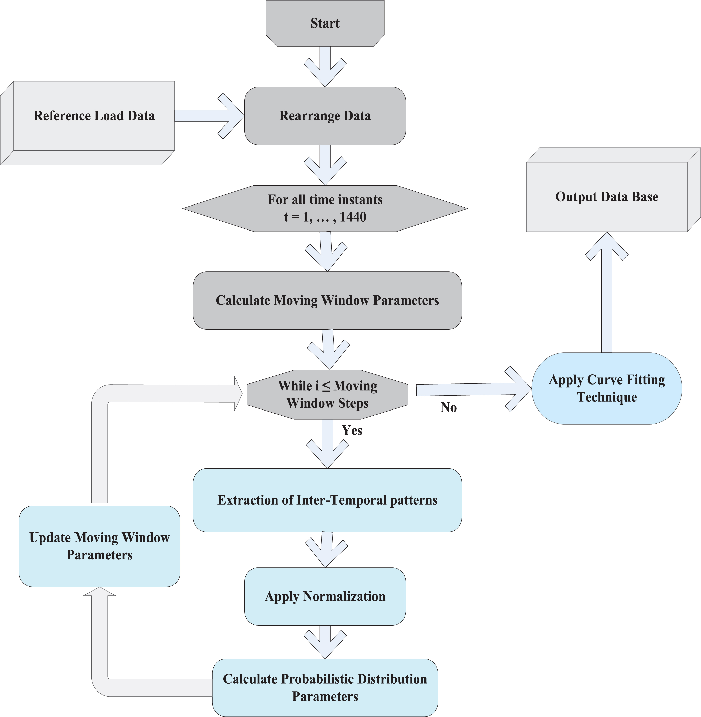
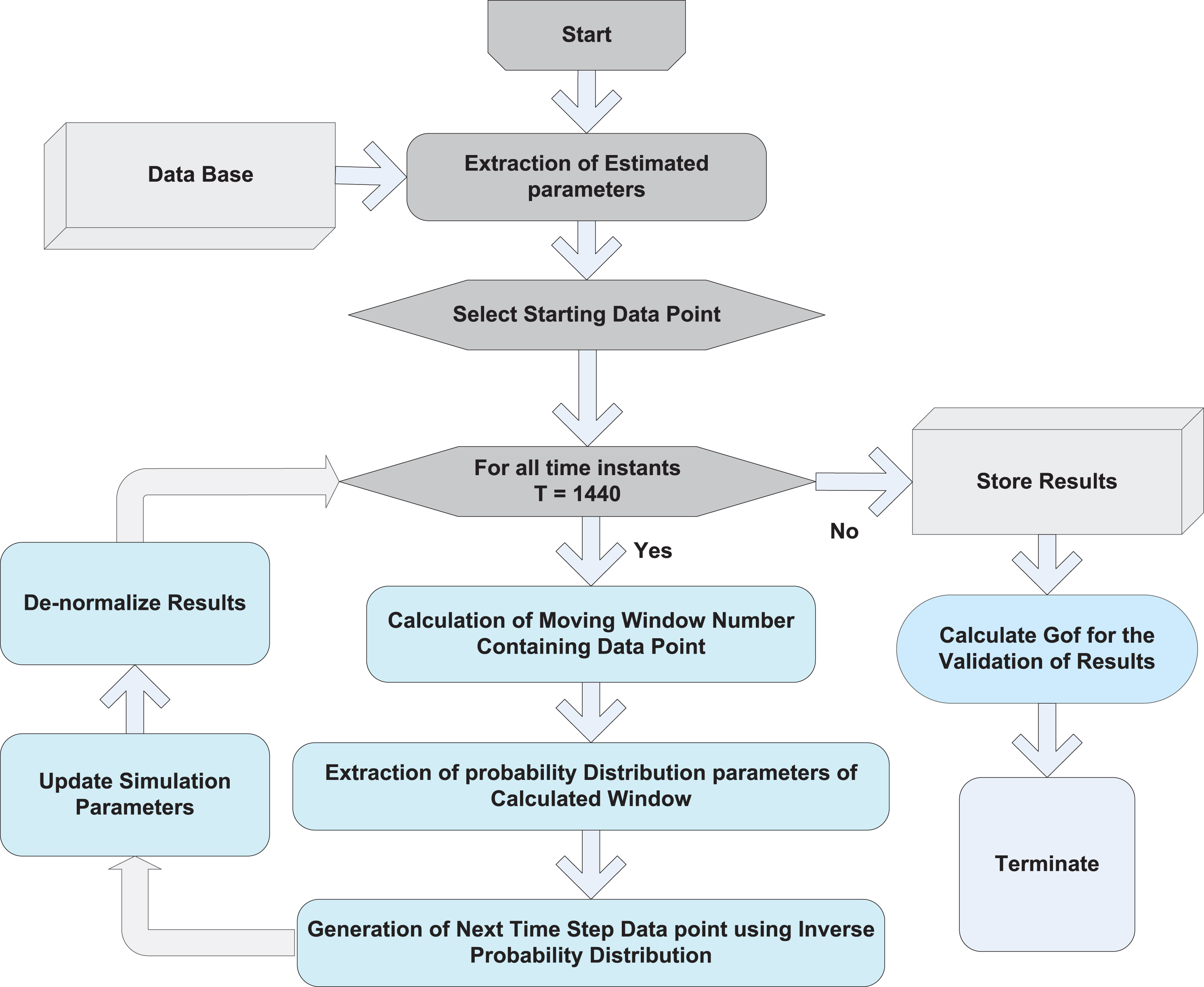
Block diagram of the proposed model for the generation of aggregate electrical demand patterns based on the estimated characteristics of reference dataset is shown in Fig. 2. This figure presents three-stage methodology for the proposed scheme. The first block outlines the procedure to extract inter-temporal change in demand characteristics using the moving window technique, which is based on Weibull distribution and GRNN. The second block depicts the generation of load pattern scenarios. The third block is about the validation part of proposed technique that uses AMAPE for calculating percentage error between reference and generated demand patterns.

Fig. 2

Flow diagram for proposed methodology.

2.2 Selection of moving window parameters

To scan the entire range of demand data for applying the probability distribution model, there is a need for an appropriate selection of moving window parameters. The lower and upper bounds of the electrical demand for 100 observations at any time step (t) and t = 1, 2 ... , T defines the starting and the ending point for which the moving window will operate and it is applied using 95% confidence interval of demand data to eliminate incorrect or bad data from aggregated demand patterns [16], as represented in (2) and (3). $d^{l} = [d \underset{1}{l} d \underset{2}{l} \dots d \underset{T}{l}]$ (2) $d^{u} = [d^{\underset{1}{u}} d^{\underset{2}{u}} \dots d^{\underset{T}{u}}]$ (3) where, d ^l and d ^u are the vectors of the upper and the lower bounds of demand data as described in (1).

The range of data ( w ^95%) for each time step can be determined as given in (4). $w^{95 %} = d^{u} - d^{l}$ (4)

The moving window of an appropriate size is selected for the extraction of demand patterns which lie inside the range. The window size can also be controlled by user defined parameter w_c.

Window width ‘ w _d’ at specific time step ‘t’ is equal to the selected range of data w ^95% at specific time step ‘t’ divided by the window size control parameter ‘ w _c’. $w_{d} = \frac{w^{95 %}}{w_{c}}$ (5)

Demand patterns at the next time step, i.e. t + 1, linking to the patterns lies inside the moving window of the previous time step are extracted that provides the information of probability distribution of the respective amplitude window. The size of the amplitude window is selected in such a way that it contains some meaningful number of demand points at time step ‘t’ to provide valuable information for the construction of probability distribution. Next moving step of the amplitude window in the vertical direction is calculated in such a way that it contains some portion of the previous window to provide smoothness in the variation of the probability distribution parameters. Shifting step of an amplitude window is calculated as mentioned in (6). $w_{s} = \frac{w^{95 %}}{w_{p} - 1}$ (6)

Where w_p is the number of central points of an amplitude window, and it should be greater than ‘ w _c’ to have an appropriate overlapping between two consecutive moving windows.

In order to extract the reference demand patterns at specific time step ‘t’, the central point of moving window lies on lower boundary of the respective time step ‘t’. Values of demand patterns occurred inside the window size $d^{l} - \frac{w_{d}}{2}$ to $d^{l} + \frac{w_{d}}{2}$ are extracted.

Demand points occurred in the next time step ‘t+1’ and linked with the extracted demand patterns of time step ‘t’ are taken out and stored in vector ‘V_t’ for specific window. An amplitude window is shifted upward by using (6). For the following step of the moving window, linking demand patterns at successive time step ‘t+1’ are extracted and stored in vector ‘V_t +1’. This process is repeated for all moving windows in vertical direction for specific time step ‘t’. For the following time step‘t+1’ same procedure is repeated for the calculation of window width‘ w _d’, window shifting step‘ w _c’ and linking demand patterns at successive time step ‘t+2’ are extracted and stored in set ‘V_t₊₁’. This procedure is repeated for all time steps, i.e., t = 1, 2 ... , T and same process is applied for the characterization of inter-temporal aggregated demand patterns for different time step durations (10, 20, 30, and 60 minutes) and aggregation levels (20, 50, 75, and 150 houses).

The above-mentioned procedure is illustrated in Fig. 3.

Fig. 3

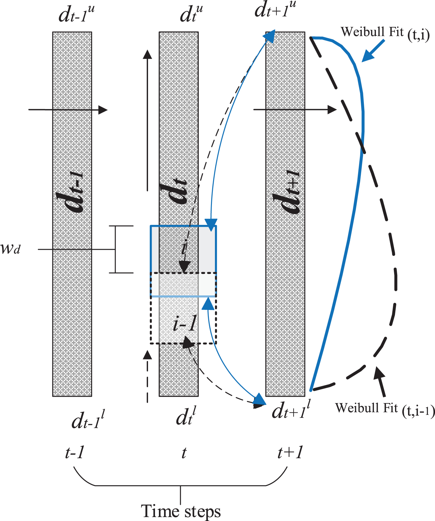
Detailed procedure for the calculation of Weibull distribution parameters.

2.3 Estimation of weibull distribution parameters

In [16], a probabilistic approach of beta distribution was used to characterize aggregate residential demand patterns. However, due to the widespread applications of Weibull distribution for uncertainty modeling (as discussed in Section 1), we choose Weibull distribution for probabilistic characterization in this paper.

Detailed flowchart related to the procedure for the extraction of Weibull distribution parameters is shown in Fig. 4. Demand patterns placed at time step ‘t+1’ linking the demand patterns of previous time step ‘t’ occurred inside the specific moving window are extracted. For moving window ‘i’, the extracted demand points lie inside the set ‘V_t,i’ are normalized using (7) in the interval (0, 1) for the estimation of shape and scale parameters. $V_{t, i} = \frac{v_{t, i} - d^{l}}{d^{u} - d^{l}}$ (7)

Fig. 4

Flowchart of the algorithm for the determination of probabilistic distribution parameters.

After normalization, shape and scale parameters of Weibull distribution are estimated for all moving windows at a specific time step ‘t’, then, the same procedure is repeated for all time steps T.

The methodology presented in this subsection generates the results on discrete steps of moving window. To have continuity in the Weibull distribution parameters, we perform curve fitting between the electrical demand and the Weibull distribution parameters.

3 Curve fitting technique

Curve fitting is a mathematical process for generating a plot that represents the discrete input data set in the continuous form. Different techniques of curve fitting have been developed which characterize the discrete input data set. Method of linear regression and arbitrage smoothing method have been discussed in [22, 23] which were used as a tool for curve fitting.

Artificial neural network is a computational model inspired by the human brain. A basic structure of artificial neural network consists of three layers: an input layer, an output layer and a middle and hidden layer consisting of a number of neurons. Each layer links with the adjacent layer through defined transfer functions. In [24], an artificial neural network has been used for curve fitting on a coarse data to accurately represent data characteristics. The proposed technique was used to predict the probability distribution curve of available coarse data and the results demonstrated that ANN perform accurately with few data points.

3.1 Generalized Regression Neural Network (GRNN)

In ANN domain, GRNN is the simplest neural network in terms of learning algorithm and network architecture. Fig. 5 shows general structure of a GRNN. In [25], performance of Back Propagation Neural Network (BPNN) and GRNN was compared and the results showed that GRNN require very less time for training and executes better results than BPNN. In [26, 27], results from GRNN and BPNN were compared and it was concluded that GRNN has high accuracy and less training time.

Fig. 5

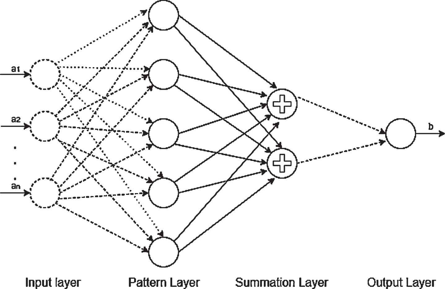
GRNN general structure.

In literature, GRNN is mostly used for for nonlinear mapping, forecasting, building a relation between inputs and outputs, estimating and self-learning application, image processing application [28, 29].

In [16], piece wise cubic hermit interpolation (PCHIP) technique was used for curve fitting. However, in this paper, GRNN is adopted for curve fitting to preserve the shape and monotonicity of the Weibull distribution scale and shape parameters due to its accuracy and effectiveness as discussed in [24, 25] and [29]. The shape and scale parameters of Weibull distribution before and after applying GRNN is shown in Fig. 6. Base formula of GRNN is given in (8). 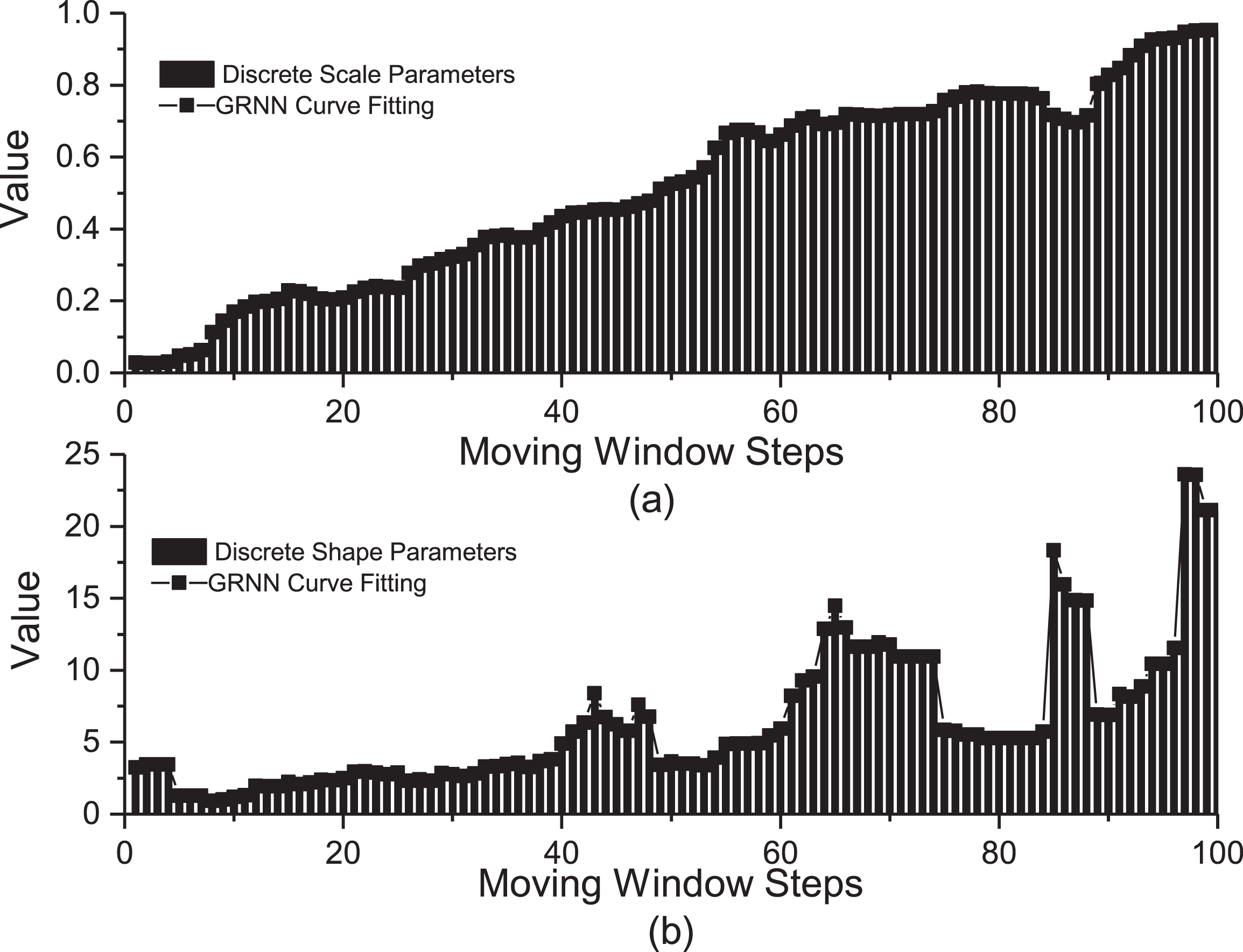$E (b / A) = \frac{\int_{- \infty}^{\infty} bf (a, b) db}{\int_{- \infty}^{\infty} f (a, b) db}$ (8)

Fig. 6

(a) Scale and (b) shape parameters of Weibull distribution before and after applying GRNN curve fitting technique on moving window at time interval 10 with 1-minute time step and 150 aggregation level.

Where ‘b’ is the estimator output, ‘a’ is the input data, E (b/A) is the output expected value, f (a, b) is the joint probability function of a and b. The detailed mathematical model of GRNN that is opted for this paper can be found in [30].

4 Scenario generation

Methodology presented in the previous section has given the Weibull distribution parameters of aggregated residential demand patterns at each time step through the probabilistic link between successive time steps of different time step durations, i.e. Δt= 1, 10, 20, 30 and 60 min. and different levels of aggregation, i.e. A = 20, 50, 75, and 150 houses. The probability distribution and inter-temporal probabilistic links are used to generate aggregate residential demand patterns, whose characteristics resemble reference demand patterns. For this purpose, a random starting demand point at time step ‘t’ is selected. Moving window step number at time step ‘t’ is calculated in which started demand point exists. Both parameters of Weibull distribution for calculated moving window are estimated from GRNN curve fitting technique at a specific time step ‘t’. Fig. 7 shows the detailed flowchart of the algorithm for scenario generation based on the estimated parameters.

Fig. 7

Flowchart of the algorithm for scenario generation based on estimated parameters.

Let η_{j
_t} and β_{j
_t} be the Weibull scale and shape parameters of starting demand pattern j_t and c_t+1 be the generated cumulative probability at time step ‘t+1’ then normalized demand point is generated by using inverse Weibull cumulative distribution function (CDF) at time step ‘t+ 1’ and is represented in the mathematical form as given in (9).

$\begin{matrix} {\tilde{j}}_{t + 1} = F^{- 1} (c_{t + 1} | η_{j_{t}}, β_{j_{t}} \\ = [{\tilde{j}}_{t + 1} : F ({\tilde{j}}_{t + 1} | η_{j_{t}}, β_{j_{t}}) = c_{t + 1}] \end{matrix}$ (9)

Where ${\tilde{j}}_{t + 1}$ is the aggregate demand point at time step‘t+1’.

Generated demand pattern ${\tilde{j}}_{t + 1}$ is de-normalized using: $j_{t + 1} = [({\tilde{j}}_{t + 1}) (d_{t}^{u} - d_{t}^{l})] + d_{t}^{l}$ (10)

Aggregate demand patterns at all time steps, t = 1, 2 ... , 1440, of specific time step duration Δt are generated by repeating above-mentioned procedure. Same process is used for the generation of aggregated demand patterns of all Δt and A.

Since ‘O’ aggregated demand observations are used in the reference data set, so same aggregated demand patterns are generated to compare the performance of the proposed model. The generated dataset is represented in (11). $J = [\begin{matrix} j_{11} & j_{12} & \begin{matrix} \dots & j_{1 T} \end{matrix} \\ j_{21} & j_{22} & \begin{matrix} \dots & j_{2 T} \end{matrix} \\ \begin{matrix} ⋮ \\ d_{O 1} \end{matrix} & \begin{matrix} ⋮ \\ d_{O 2} \end{matrix} & \begin{matrix} \begin{matrix} ⋮ \\ \dots \end{matrix} & \begin{matrix} ⋮ \\ d_{OT} \end{matrix} \end{matrix} \end{matrix}]$ (11)

5 Case study

The reference data sets of aggregated demand patterns used in this study has been presented in [7] and [16]. The reference demand pattern data set consists of 4 aggregation levels and 5 different time step duration, of residential customers for winter weekdays. Reference data consists of 100 observations for a typical winter weekday. The reference data of time step duration Δt= 1 minute for all the aggregation levels, A = 20, 50, 75 and 150, is shown in Fig. 1. Table 1 shows the parameter used for initialization of the proposed method in this study.

Table 1
Scenario generation model parameters

Sr. # Parameters Value

1. Aggregation Levels (A) 20, 50, 75, 150 houses

2. Time Step Durations (Δt) 1, 10, 20, 30, 60 min.

3. No of Window Steps (w_p) 100

4. Window Size Control 10

Parameter (w_c)

Sr. #	Parameters	Value
1.	Aggregation Levels (A)	20, 50, 75, 150 houses
2.	Time Step Durations (Δt)	1, 10, 20, 30, 60 min.
3.	No of Window Steps (w_p)	100
4.	Window Size Control	10
Parameter (w_c)

For the calculation of Weibull distribution scale and shape parameters, the detail algorithm presented in Fig. 4 is used. GRNN based curve fitting technique is applied to achieve the continuity of Weibull distribution parameters and the results are shown in Fig. 6.

The extracted Weibull distribution parameters are then used to generate different scenarios of aggregated demand patterns whose characteristics resembles reference demand patterns. The complete flowchart of the procedure for generating scenarios is shown in Fig 7. In scenario generation, inter-temporal variations of generated demand patterns should be similar to the reference demand patterns.

5.1 Goodness of Fit (GOF) Assessment

Comparison of mean and standard deviation of generated dataset with the load patterns generated using Beta distribution and reference data is shown in Fig. 8. It can be seen that the mean value is almost the same in all three cases. However, for standard deviation, the performance of proposed Weibull distribution-based method is largely closer to the reference data and outperforms the Beta distribution-based method. To further validate this conclusion, the accuracy of the proposed model is calculated by using well-known goodness of fit (GOF) indicator, i.e. AMAPE, which gives the error between generated demand patterns and reference demand patterns. In literature, different other indicators such as Mean Absolute Percentage Error (MAPE), Mean Square Error (MSE) have also been used to calculate error between actual and estimated values. But, in case of smaller actual value, these indicators show large error term even if difference between estimated and actual value is small [31]. To avoid this effect AMAPE is used in this paper to calculate percentage error. This indicator is applied on the standard deviation and mean of the aggregate reference and generated demand patterns. Moreover, to assess the uncertainty of the proposed probabilistic model variance of AMAPE is also computed. Same indicators have been used in different literature to validate results as given in [16 , 32].

Fig. 8

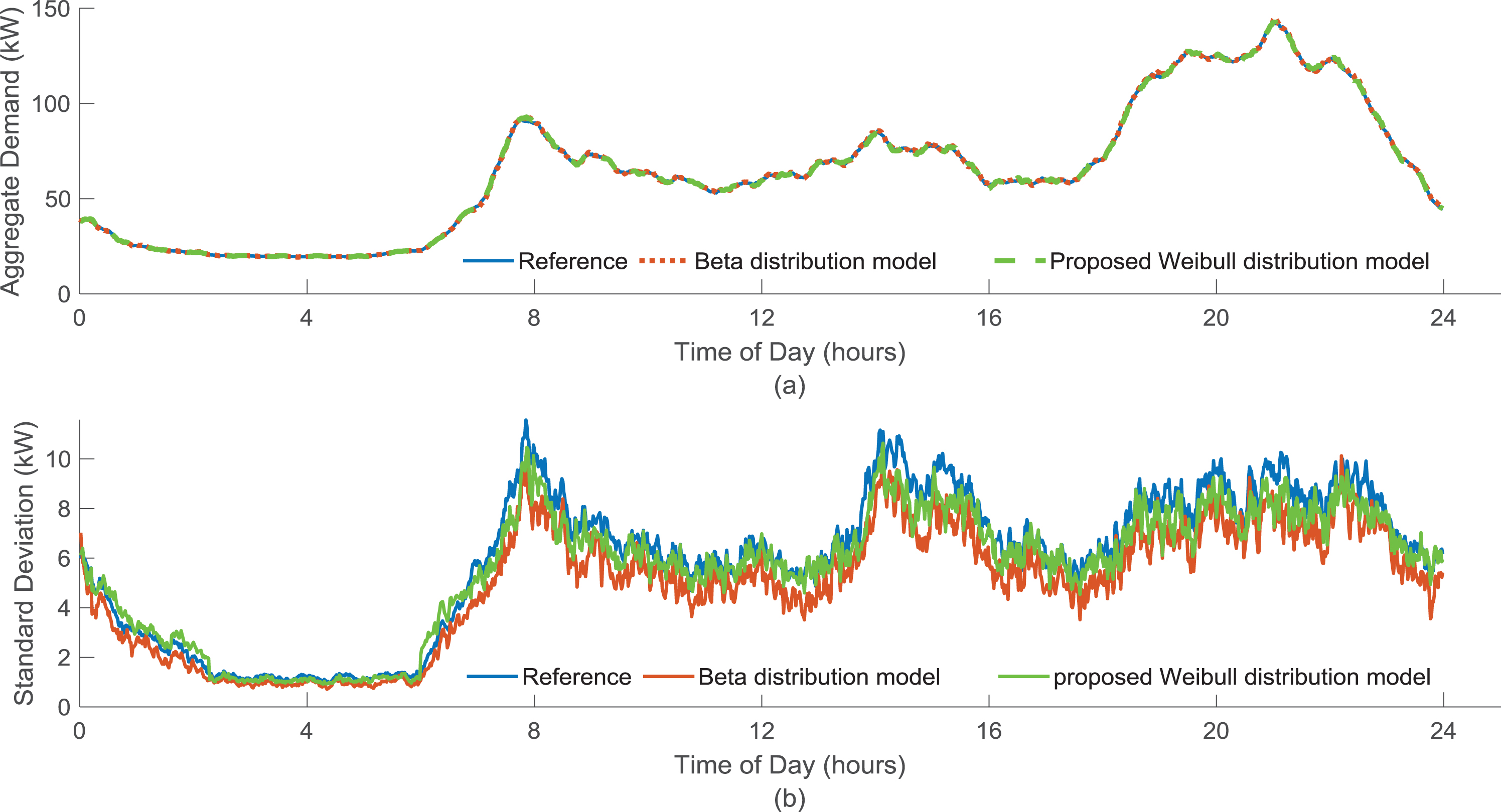
Comparison of (a) mean and (b) standard deviation for generated demand patterns with the results of Beta distribution model [16] and reference data.

Mathematical formulation for AMAPE is given in (12). $AMAPE = \frac{1}{P} (\sum_{t = i}^{i + P} [\frac{| G_{t} - R_{t} |}{(\frac{1}{P} \sum_{t = i}^{i + P} R_{t})}]) X 100$ (12)

Where P is the averaging time period to calculate AMAPE. For this paper, P = 60 minutes is assumed which was also used in [16]. G_t and R_t represent the mean or standard deviation of the generated and reference datasets respectively.

Similarly, to measure the uncertainty of scenario-generation model, variance of AMAPE is used and its mathematical expression is given in (13).

$\begin{matrix} AMAPE Variance = \frac{1}{P} \\ (\sum_{t = i}^{i + P} {[\frac{| G_{t} - R_{t} |}{(\frac{1}{P} \sum_{t = i}^{i + P} R_{t})} - \frac{AMAPE}{100}]}^{2}) X 100 \end{matrix}$ (13)

The proposed Weibull distribution probabilistic model and the beta distribution probabilistic model is applied on 1, 10, 20, 30 and 60 min time step durations and 20, 50, 75 and 150 aggregation levels. The results and percentage improvements of proposed model for the mean and standard deviation of AMAPE and AMAPE Variance σ² are shown in Fig. 9 and Fig. 10.

Fig. 9

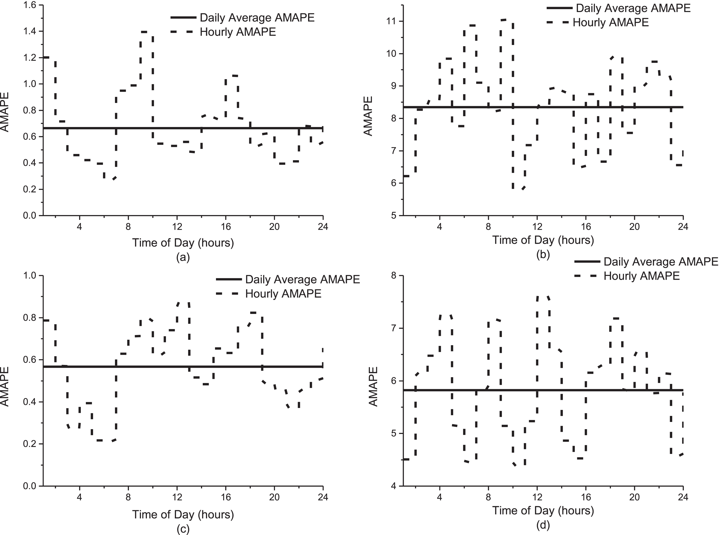
Detailed hourly AMAPE of (a) mean and (b) standard deviation of beta probabilistic model and (c) mean and (d) standard deviation of Weibull probabilistic model.

Fig. 10

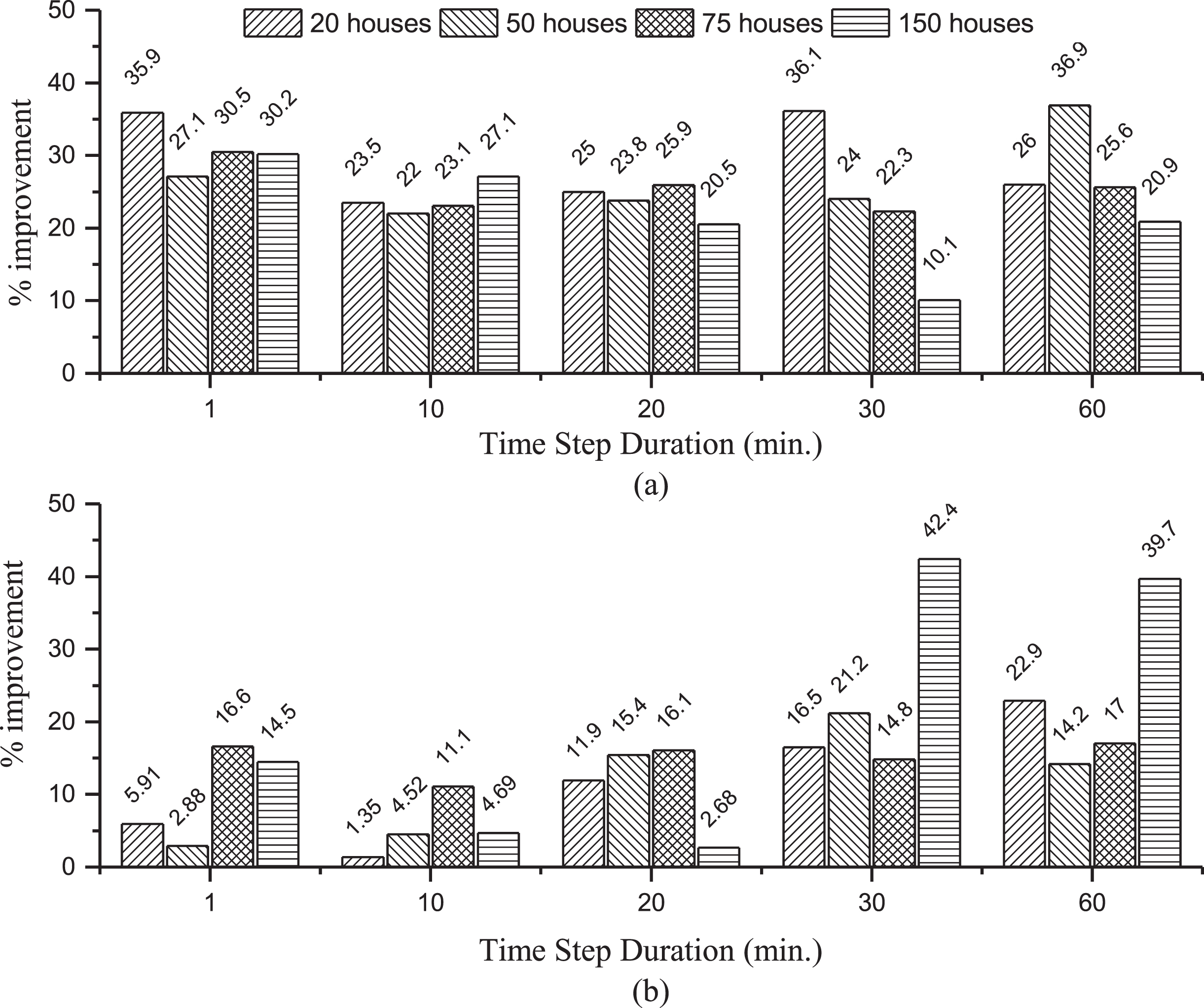
Percentage improvement in AMAPE for (a) standard deviation (b) mean in comparison with [16] for different aggregation levels and time step durations.

5.2 Analysis of one-minute time step duration

Results of AMAPE and AMAPE Variance for the mean or standard deviation of the generated and reference datasets with one minute time step duration and different aggregation levels (20, 50, 75 and 150 houses) are presented in Table 2. In [16], average value of AMAPE for one minute and 150 aggregation level was 0.64 whereas, for the proposed Weibull distribution probabilistic model, this error is 0.56. Percentage improvement of Weibull distribution model for one minute and 150 aggregation level is 14.5% and it is clearly shown in Fig. 9.

Table 2
Mean and standard deviation of AMAPE and AMAPE Variance

Aggregation Level (houses) Technique AMAPE AMAPE Variance

Average % Imp. Average % Imp. Average % Imp. Average % Imp.

Mean STD Mean STD

20 Beta [16] 1.8126 5.91 10.4788 35.9 0.0346 1.73 0.4268 44.4

Weibull 1.7053 6.7088 0.0340 0.2371

50 Beta [16] 1.0308 2.88 9.1335 27.1 0.0069 20.3 0.2785 23.1

Weibull 1.0011 6.6628 0.0061 0.1972

75 Beta [16] 0.9732 16.6 8.8789 30.5 0.0061 32.7 0.2753 20.8

Weibull 0.8118 6.1633 0.0041 0.2180

150 Beta [16] 0.6640 14.5 8.3496 30.2 0.0025 20 0.2649 31.1

Weibull 0.5675 5.8219 0.0020 0.1824

Aggregation Level (houses)	Technique	AMAPE	AMAPE Variance
20	Beta [16]	1.8126	5.91	10.4788	35.9	0.0346	1.73	0.4268	44.4
	Weibull	1.7053		6.7088		0.0340		0.2371
50	Beta [16]	1.0308	2.88	9.1335	27.1	0.0069	20.3	0.2785	23.1
	Weibull	1.0011		6.6628		0.0061		0.1972
75	Beta [16]	0.9732	16.6	8.8789	30.5	0.0061	32.7	0.2753	20.8
	Weibull	0.8118		6.1633		0.0041		0.2180
150	Beta [16]	0.6640	14.5	8.3496	30.2	0.0025	20	0.2649	31.1
	Weibull	0.5675		5.8219		0.0020		0.1824

Standard deviation of AMAPE for one minute time step duration and aggregation of 150 houses as calculated in [16] using beta probability distribution model was 8.54 whereas for the proposed method it is 5.82. Percentage improvement of standard deviation for one minute and 150 houses aggregation is 30.2%.

Detailed results of AMAPE and its Variance are listed in Table 3.

Table 3

Detailed results of mean and standard deviation of AMAPE and AMAPE Variance of 150 Aggregation at 1-minute time step duration.

GOF index	Parameter	Probabilistic Model Values
		Max.		Min.		Average
		Beta [16]	Weibull	Beta [16]	Weibull	Beta [16]	Weibull
AMAPE	Mean	1.39	0.87	0.27	0.21	0.66	0.56
	STD	11.05	7.61	5.85	4.38	8.54	5.82
AMAPE Variance	Mean	0.01	0.004	0	0	0.0025	0.002
	STD	0.40	0.38	0.13	0.09	0.26	0.18

Maximum values of AMAPE for mean and standard deviation with one minute time step duration and 150 houses aggregation level were 1.39 and 11.05 respectively as calculated using beta probabilistic model and reported in [16]. Whereas, the maximum values of AMAPE for mean and standard deviation calculated using Weibull distribution based model are 0.87 and 7.61 respectively. Similarly, minimum values calculated using beta distribution model are 0.27 and 5.85 while the minimum value of Weibull distribution model is 0.21 and 4.38.

AMAPE Variance for mean and standard deviation calculated using beta distribution model were 0.0025 (approximately zero) and 0.26 [16]. The respective values calculated using Weibull distribution model are 0.002 and 0.18. Percentage improvement of mean and standard deviation is 20% and 31.1% respectively.

AMAPE Variance for mean and standard deviation is calculated for all aggregation levels and time step durations using beta probability distribution model and Weibull distribution based model. Percentage improvement of Weibull distribution model with respect to beta probabilistic model is shown in Fig. 10. It can be noted that Weibull distribution with GRNN is more effective to model inter-temporal change in demand characteristics. In addition to this, it can also be observed that the performance of the proposed method is better than beta distribution model for different time step durations and demand aggregation levels. The results dictate that this methodology can equally be applied for scenario generations at different customer aggregations with changing time step duration.

6 Conclusions

In this paper, a new probabilistic model based on Weibull distribution and GRNN has been presented for the inter-temporal characterization of aggregate demand to generate different scenarios based on reference daily load patterns of residential customers. Proposed probabilistic model has been applied on datasets with 1, 10, 20, 30 and 60 minutes of time step duration and 20, 50, 75 and 150 houses aggregation levels. Well known goodness of fit (GOF) techniques have been used for the evaluation of proposed probabilistic model. GOF indicators have validated the accuracy of the Weibull distribution model. Results for the mean and standard deviation of AMAPE and AMAPE Variance show the effectiveness of the proposed model. Moreover, existing methods for the characterization of aggregate demand pattern are supported by this research. This research work can further be extended to the construction of renewable power generation scenarios and power difference patterns between generation and electric demand in a microgrid environment.

References

Torriti

, Understanding the timing of energy demand through time use data: Time of the day dependence of social practices, Energy Research & Social Science 25 (2017), 37–47.

Gottwalt

, Gärttner

, Schmeck

and Weinhardt

, Modeling and valuation of residential demand flexibility for renewable energy integration, IEEE Transactions on Smart Grid 8 (2017), 2565–2574.

Chicco

, Napoli

, Postolache

, Scutariu

and Toader

, Customer characterization options for improving the tariff offer, IEEE Transactions on Power Systems 18 (2003), 381–387.

Sajjad

I.A.

, Chicco

and Napoli

, Effect of aggregation level and sampling time on load variation profile—A statistical analysis, in Mediterranean Electrotechnical Conference (MELECON), 2014 17th IEEE, 2014, pp. 208–212.

Sajjad

I.A.

, Chicco

and Napoli

, A probabilistic approach to study the load variations in aggregated residential load patterns, in Power Systems Computation Conference (PSCC), 2014, 2014, pp. 1–7.

Zhou

, Yang

and Shen

, Discovering residential electricity consumption patterns through smart-meter data mining: A case study from China, Utilities Policy 44 (2017), 73–84.

Cagni

, Carpaneto

, Chicco

and Napoli

, Characterisation of the aggregated load patterns for extraurban residential customer groups, in Electrotechnical Conference, 2004. MELECON 2004. Proceedings of the 12th IEEE Mediterranean, 2004, pp. 951–954.

Tho

K.K.

, et al., Artificial neural network model for material characterization by indentation. Modelling and simulation, Materials Science and Engineering 12(5) (2004), 1055.

Beucher

, Siemssen

, Fröjdö

, Österholm

, Martinkauppi

and Edén

, Artificial neural network for mapping and characterization of acid sulfate soils: Application to Sirppujoki River catchment, southwestern Finland, Geoderma 247–248 (2015), 38–50. Doi: 10.1016/j.geoderma.2014.11.031

10.

Yen

, Chang

, Hsu

and Liu

, Artificial Neural NetworkModel forMass Characterization in Breast Palpation, IEEE International Conference on Systems, Man and Cybernetics, Taipei, 2006, 507–512.

11.

Ascione

, Bianco

, De Stasio

, Mauro

G.M.

and Vanoli

G.P.

, Artificial neural networks to predict energy performance and retrofit scenarios for any member of a building category: A novel approach, Energy 118 (2017), 999–1017.

12.

Beccali

, Ciulla

, Brano

V.L.

, Galatioto

and Bonomolo

, Artificial neural network decision support tool for assessment of the energy performance and the refurbishment actions for the non-residential building stock in Southern Italy, Energy 137 (2017), 1201–1218.

13.

Akyuz

A.O.

, Uysal

, Bulbul

B.A.

and Uysal

M.O.

, Ensemble approach for time series analysis in demand forecasting: Ensemble learning, in INnovations in Intelligent SysTems and Applications (INISTA), 2017 IEEE International Conference on, 2017, 7–12.

14.

Son

and Kim

, Short-term forecasting of electricity demand for the residential sector using weather and social variables, Resources, Conservation and Recycling 123 (2017), 200–207.

15.

Dang-Ha

T.-H.

, Bianchi

F.M.

and Olsson

, Local short term electricity load forecasting: Automatic approaches, in Neural Networks (IJCNN), 2017 International Joint Conference on, 2017, 4267–4274.

16.

Sajjad

I.A.

, Chicco

and Napoli

, Probabilistic generation of time-coupled aggregate residential demand patterns, IET Generation, Transmission & Distribution 9 (2015), 789–797.

17.

Saat

N.M.Z.

, Jemain

A.A.

and Al-mashoor

S.H.A

, A Comparison of Weibull and Gamma Distribution in Application of Sleep Apnea, Asian Journal of Mathematics and Statistics 1(3) (2008), 132–138.

18.

Afzaal

M.U.

, Sajjad

I.A.

and Martirano

, Weibull Distribution Model for the Characterization of Aggregate Load Patterns, 2018 IEEE International Conference on Environment and Electrical Engineering and 2018 IEEE Industrial and Commercial Power Systems Europe (EEEIC / I&CPS Europe), Palermo, 2018, 1–5.

19.

Labeeuw

and Deconinck

, Customer sampling in a smart grid pilot, in Power and Energy Society General Meeting, 2012 IEEE, 2012, 1–7.

20.

Spech

D.F.

, A General Regression Neural Network, IEEE Transactions On Neural Networks 2(6) (1991).

21.

Theodosiou

, Disaggregation & aggregation of time series components: A hybrid forecastingapproach using generalized regression neural networks and the theta method, Neurocomputing 74(1) (2011).

22.

Cleveland

W.S.

and Devlin

S.J.

, Locally weighted regression: an approach to regression analysis by local fitting, Journal of the American Statistical Association 83 (1988), 596–610.

23.

Desmet

and Gijbels

, Curve fitting under jump and peak irregularities using local linear regression, Communications in Statistics-Theory and Methods 40 (2011), 4001–4020.

24.

Balasubramanyam

, Ajay

, Spandana

, Shetty

A.B.

and Seetharamu

, Curve fitting for coarse data using artificial neural network, WSEAS Transaction on Mathematics 13 (2014), 406–415.

25.

del Rosario Martínez-Blanco

, et al., A comparison of back propagation and Generalized Regression Neural Networks performance in neutron spectrometry, Applied Radiation and Isotopes 117 (2016), 20–26.

26.

Zhang

X.H.

, et al., Application of general regression neural network to the prediction of LOD change, Chinese Astronomy and Astrophysics 36(1) (2012), 86–96.

27.

Al-Mahasneh

A.J.

, Anavatti

S.G.

and Garratt

M.A.

, Review of Applications of Generalized Regression Neural Networks in Identification and Control of Dynamic Systems, arXiv preprint arXiv:1805.11236, 2018.

28.

Liu

, Jia

, Kong

, Guan

and Zhang

, Artificial neural network application to study quantitative relationship between silicide and fracture toughness of Nb-Si alloys, Materials & Design 129 (2017), 210–218.

29.

Mandal

, Sivaprasad

, Venugopal

, Murthy

and Raj

, Artificial neural network modeling of composition–process–property correlations in austenitic stainless steels, Materials Science and Engineering: A 485 (2008), 571–580.

30.

Feng

, Peng

, Cui

, Gong

and Zhang

, Modeling reference evapotranspiration using extreme learning machine and generalized regression neural network only with temperature data, Computers and Electronics in Agriculture 136 (2017), 71–78.

31.

and Shahidehpour

, A hybrid model for day-ahead price forecasting, IEEE Trans. on Power Syst 25(3) (2010), 1519–1530.

32.

Khan

M.F.N.

, Malik

T.N.

and Sajjad

I.A.

, A novel probabilistic generation model for grid connected PV based distributed generation, Journal of Engineering Research 8(1) (2020), 231–247.

Inter-temporal characterization of aggregate residential demand based on Weibull distribution and generalized regression neural networks for scenario generations

Abstract

Keywords

1 Introduction

2 Data organization and mathematical framework

3.1 Generalized Regression Neural Network (GRNN)

Table 1 Scenario generation model parameters Sr. # Parameters Value 1. Aggregation Levels (A) 20, 50, 75, 150 houses 2. Time Step Durations (Δt) 1, 10, 20, 30, 60 min. 3. No of Window Steps (w p ) 100 4. Window Size Control 10 Parameter (w c )

References

Table 1
Scenario generation model parameters

Sr. # Parameters Value

1. Aggregation Levels (A) 20, 50, 75, 150 houses

2. Time Step Durations (Δt) 1, 10, 20, 30, 60 min.

3. No of Window Steps (w_p) 100

4. Window Size Control 10

Parameter (w_c)