Nonlinear system modeling using the takagi-sugeno fuzzy model and long-short term memory cells

Abstract

The data driven black-box or gray-box models like neural networks and fuzzy systems have some disadvantages, such as the high and uncertain dimensions and complex learning process. In this paper, we combine the Takagi-Sugeno fuzzy model with long-short term memory cells to overcome these disadvantages. This novel model takes the advantages of the interpretability of the fuzzy system and the good approximation ability of the long-short term memory cell. We propose a fast and stable learning algorithm for this model. Comparisons with others similar black-box and grey-box models are made, in order to observe the advantages of the proposal.

Keywords

LSTM fuzzy neural networks nonlinear system identification

1 Introduction

The model of a system is the representation of the structure (properties) of the system, the choice of how a model is developed depends on what is expected to be represented in it. Obtaining models can be done in different ways, such as through physical laws (mathematical modeling); it is the most common form, but this type of technique needs knowing exactly the environment in which the system operates, as well as making the biggest amount of theoretical considerations as possible. Another way to obtain models is through measurements of aspects of interest from the system (black-box models), or such measurements together with some equations that describe the system behavior (gray-box models), achieving high robustness and adaptability. Neural networks (NNs) and fuzzy systems are very common to use as black-box models and gray-box models, respectively. The NNs and fuzzy systems can generate models by learning processes, either for system modeling or adaptive control.

Fuzzy models use fuzzy rules of the IF-THEN type to identify systems. There are two main types of fuzzy models, Mamdani fuzzy systems and Takagi-Sugeno (TS) fuzzy systems, with several comparisons between them showing that TS fuzzy systems are better for engineering tasks such as the modeling and control of systems [1]. Fuzzy systems represents experts knowledge, but they can be constructed in such a way that they emulate an expert through learning processes (like a NN) resulting in an ANFIS (adaptive network based fuzzy inference system) [2]. The ANFIS systems are based on a TS fuzzy system and transform fuzzy systems into something similar to NNs. TS models with ANFIS training are very powerful in wide range of scientific fields, such as in energy field [3] and economic decision [4].

If the consequences (THEN parts) of a TS fuzzy system are taken as nonlinear functions, it is possible to obtain better results in the general performance of the fuzzy system [5, 6]. The inclusion of NNs of different types in ANFIS systems was introduced and discussed in many works, generating fuzzy-neural or neuro-fuzzy models [7 –9]. More recent works on this topic propose RNNs to estimate the consequences in fuzzy systems (to approach a nonlinear function in each consequent part), for example the wavelet network (WN) are very suitable for this task [10]. In [31] different types of fuzzy systems are analyzed and compared to each other; these fuzzy systems are structured with conventional representations and with NNs and, according to this work, the construction of a fuzzy system depends essentially for which application it will be used. However, the approximation accuracies of the above TS models are not satisfied.

Recently a deep learning model, named long-short term memory (LSTM), has been developed [11 –14]. It has a recurrent structure and is based on information management through gates, these gates measure the suitability of the data they receive as input data, the stored data by the LSTM and the data generated by the LSTM as result. LSTM networks overcome many disadvantages of RNNs and they converge relatively faster [15 –18]. Some training algorithms specifically for LSTM networks have been proposed, to further improve their performance [19]. But as a disadvantage, the internal structure of a LSTM is more complex than the conventional RNNs. The use of deep LSTM networks is still under development, as well as their use with other intelligent systems like the fuzzy systems. For example, in the robotics field and specifically in the medical robotics some fuzzy-neural networks that includes LSTM networks are proposed to control surgeon robots [20, 21], other important applications that includes LSTM networks and fuzzy systems are the management of resources, like the management of electrical energy [22]; but in these proposals the LSTM networks and fuzzy systems work in a decoupled way.

Among the simplest ways to adjust the parameters of NNs are supervised learning algorithms, highlighting the back propagation (BP) algorithm. The BP is one of the most popular algorithms to train NNs because of its simplicity [24]. Recurrent NNs (RNNs) are the most used to model systems, because they can generate relatively fast system models, for both linear and nonlinear systems [26]. Variations of the BP algorithm have been developed to be able to adjust the parameters of RNNs efficiently, stand out the back propagation through time algorithm (BPTT) [25]. By analyzing the stability of RNNs, these networks can deal with the problem of noise and disturbances [27]. This last network represents that conventional RNNs can be changed into more complex structures in order to obtain better results as the case may be.

In order to create a network that reacts faster and with a better approximation, specially for applications in real time related to the identification and control of systems, in this paper, we make the following contributions:

We propose a novel TS fuzzy model, which employes the LSTM networks inside the structure of the fuzzy system. This model is established by the fuzzy system and benefited by the LSTM network estimation.

A learning process for this fuzzy-network is proposed, it performs in a short period of time and it is feasible. The stability of the proposed model taking into account the training algorithm is proved.

To show the advantages of the novel fuzzy LSTM network, comparisons between the proposal and other intelligent algorithms are made by using the Mackey-Glass time series and a nonlinear benchmark system. These comparatives are made to show that: 1) the novel model has better modeling performances than the other algorithms; 2) the proposed method has fast convergence and it can achieve easily the assigned task.

2 Fuzzy modeling using LSTM cells

A system can be represented as a nonlinear function in discrete time as follows: $y (k) = φ [U_{r} (k)]$ (1) where φ (·) is an unknown nonlinear difference equation, also the state vector U_r (k) is defined as: $\begin{matrix} [c] c U_{r} (k) = [y (k - 1), \dots, y (k - n_{y}), u (k), \dots \\ \dots, u (k - n_{u})]^{T} = {[u_{r_{1}} \dots u_{r_{m}}]}^{T} \end{matrix}$ (2) with u (k) and y (k) as the input and the output signals for the system, n_y indicates the number of the delayed output signal, n_u indicates the number of the delayed input signal, and m indicates the number of elements u_{r
_m} in U_r (k).

The representation shown in (1) and (2) is known as a NARMA model. To model that system, we use fuzzy IF-THEN rules similar to a conventional TS fuzzy system, then for the p-th rule it has: $\begin{matrix} [c] c R_{p} : IF u_{r_{1}} (k) IS A_{1 p} & u_{r_{2}} (k) IS A_{2 p} & \dots \\ \dots & u_{r_{m}} (k) IS A_{jp}, THEN h_{p} (k) = ϱ_{p} (k) \end{matrix}$ (3) where h_p (k) is an estimation to the function ϱ_p (k) that represents the consequent part of each fuzzy rule. The sets A_jp, with j = 1 … κ, are the fuzzy sets for the fuzzification (using κ fuzzy sets) of each u_{r
_m} in (2).

The membership functions associate to each A_jp are described as follows: $μ_{A_{jp}, u_{r_{m}}} (k) = exp (- \frac{{(u_{r_{m}} (k) - ς_{jp})}^{2}}{2 ν_{jp}})$ (4) In this Gaussian function, the center is $ς_{jp} \in ℝ$ and the width is $ν_{jp} \in ℝ^{+}$ . For the final estimation of a system, the contribution of each input element to the premise part (IF part) of a fuzzy rule in (3) is obtained by the T-norm, $z_{p} (k) = \prod_{j = 1}^{κ} μ_{A_{jp}, u_{r_{m}}} (k)$ (assuming j = m).

A more general representation of the value of each element of (4) in each fuzzy set can be done in a vectorial way: $ζ_{j} = exp [{(U_{r} (k) - χ_{j})}^{2} \otimes (- \frac{1}{2} ϒ_{j})]$ (5) with χ_j, $ϒ_{j} \in ℝ^{m}$ as the center and width vectors for $ζ_{j} \in ℝ^{m}$ , respectively. The vector ζ_j represents the value of each element of u_{r
_m} (k) in fuzzy set A_j, and ⊗ is the operator for the element to element product in vectors. This representation will be useful for the adjustment of the parameters of the fuzzy-network.

The consequent part (THEN part) of one fuzzy rule in (3) is represented by h_p (k). The function h_p (k) usually is defined as a linear combination of the inputs signals (2) of the system (1), but as was said in the introduction, better estimations are achieve with the use of nonlinear functions (with the input signals as arguments); this nonlinear functions can be easily obtained by a NNs, and one of the best to do this is a LSTM cell. However, when n_y and n_u in (2) are unknown, i.e., we do not known how long the current status depends on their previous information, especially when the time series is long, the information between the relevant and place becomes smaller and smaller. So we need a model which can hands the “long-term dependencies”, and LSTM cells has this property.

The estimation of (1) is obtained by the defuzzification of the fuzzy system (3) with p rules: $\hat{y} (k) = \frac{\sum_{n = 1}^{p} z_{n} h_{n} (k)}{\sum_{n = 1}^{p} z_{n}} = \sum_{n = 1}^{p} {\bar{z}}_{n} h_{n} (k)$ (6) where: ${\bar{z}}_{p} = z_{p} / (z_{1} + z_{2} + \dots + z_{n})$ The premise can be represented in a vectorial way as $Z_{F} \in ℝ^{p}$ , where all the elements of this new vector are the organized multiplications as was explained in (4). Also, each element of Z_F is normalized as in (6). For multiple estimations, the elements of Z_F can be organized in such a way that the premise parts repeats for every estimation, hence the consequent parts are the only ones that are different for several estimation in a same system.

The concept of the fuzzy system using the LSTM cells is shown in Fig. 1, and it is divided in 4 layers: in the first layer the inputs of the network are organized, in the second layer this inputs are fuzzificated, in the third layer the values of the IF and THEN parts are calculated, and in the fourth layer the estimation of the system is made according to (6).

Fig. 1

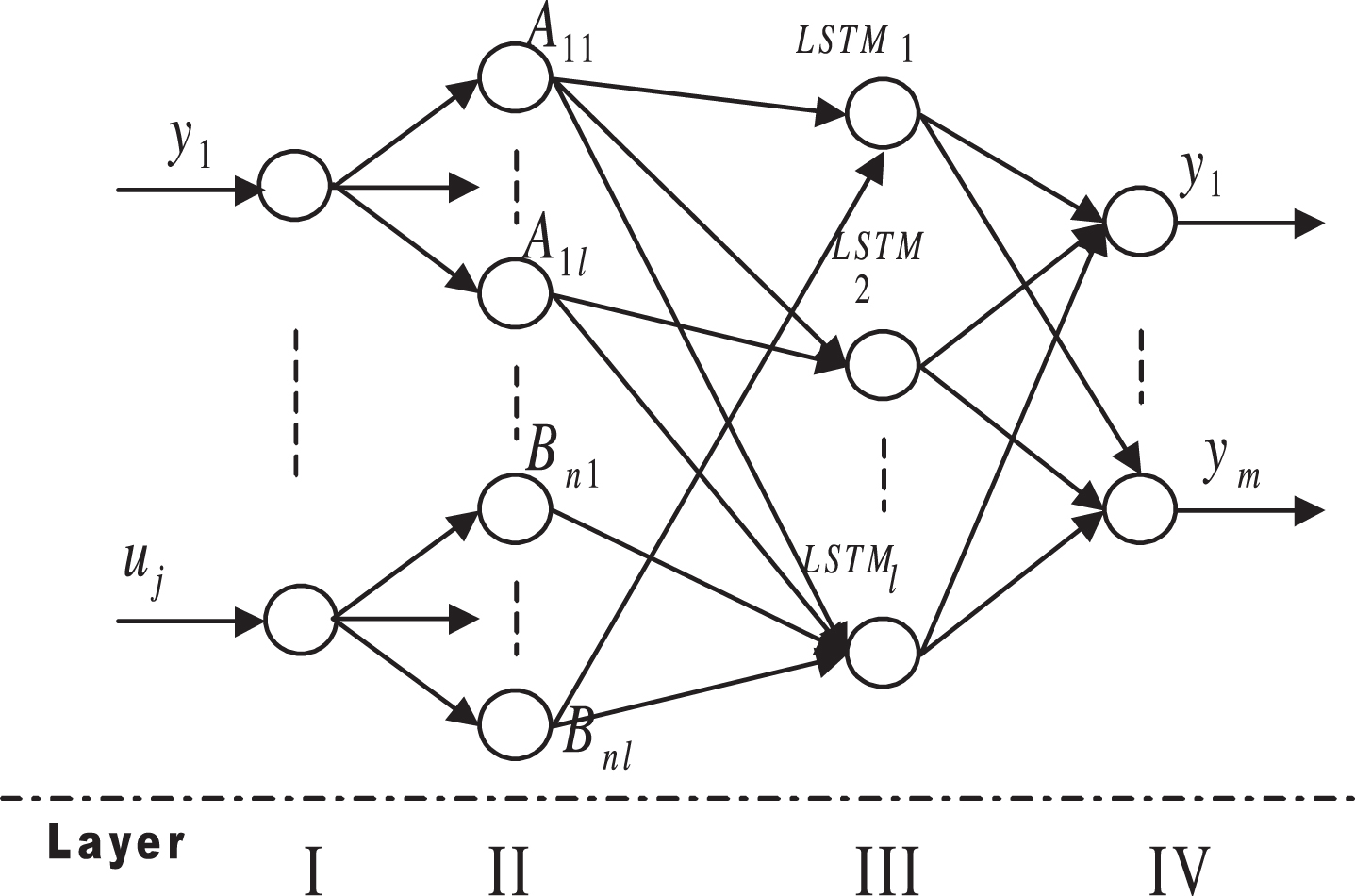
Fuzzy model with LSTM cells.

So, the LSTM cells in the consequent part is shown in Fig. 2. The cells process data using the “gate” technique to let useful information pass through its structure. This cell is capable of handling long-term and short-term data dependencies in more efficient way than a conventional RNN. The cells can work together, as a network and also can be organized as an array.

Fig. 2

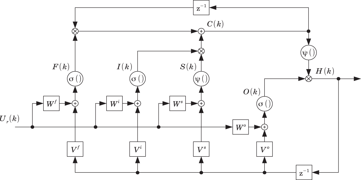
LSTM cell for the consequent part.

The LSTM network has several stages, which are describe by: $F (k) = σ (W^{f} U_{r} (k) + V^{f} H (k - 1))$ (7) $I (k) = σ (W^{i} U_{r} (k) + V^{i} H (k - 1))$ (8) $S (k) = ψ (W^{s} U_{r} (k) + V^{s} H (k - 1))$ (9) $C (k) = F (k) \otimes C (k - 1) + I (k) \otimes S (k)$ (10) $O (k) = σ (W^{o} U_{r} (k) + V^{o} H (k - 1))$ (11) $H (k) = O (k) \otimes ψ (C (k))$ (12) where: F (k), I (k), S (k), C (k), O (k) and $H (k) \in ℝ^{p}$ are sections of the network, they are: the fitness of the internal state, the fitness of the internal input, the internal input, the internal state, the fitness of the output, and he output of the LSTM network, respectively. The synaptic weights are: W^f, Wⁱ, W^s and $W^{o} \in ℝ^{p \times m}$ ; V^f, Vⁱ, V^s and $V^{o} \in ℝ^{p \times p}$ as diagonal matrices or V^f, Vⁱ, V^s and $V^{o} \in ℝ^{p}$ as vectors, according to the need. The functions σ (·) and ψ (·) are the sigmoid and hyperbolic tangent functions, respectively, $U_{r} (k) \in ℝ^{m}$ is the input in (2).

From (6), the output of the fuzzy system is $\hat{y} (k) = Z_{F} H (k)$ (13) where H (k) = [h₁ (k) ⋯ h_p (k)] ^T corresponds to the THEN parts, $Z_{F} \in ℝ^{n}$ is the elements of the IF parts. The number of LSTM cells, as well as the number of fuzzy rules, are defined as p = κ^m for the case of 1 estimation, for several estimations it has p = l (κ^m) where l is the number of estimations (thus $\hat{y} \in ℝ^{l}$ ), as was described for (6).

According to function approximation theories of fuzzy systems [28], the identified nonlinear process (1) can be represented as: $Y (k) = Z_{F} (W^{*}) H (W^{*}) + μ (k)$ (14) where W^∗ is the unknown weights which can minimize the unmodeled dynamic μ (k). The identification error: $e (k) = \hat{y} (k) - y (k)$ (15) can be represented by (13) and (14) $e (k) = Z_{F} (\tilde{W}) H (\tilde{W}) + μ (k)$ (16) where $Z_{F} (\tilde{W}) H (\tilde{W}) = Z_{F} (W^{*}) H (W^{*}) - Z_{F} H (k)$ $\tilde{W} (k) = W (k) - W^{*}$ . In this paper we are only interested in open-loop identification, we assume that the plant (1) is bounded-input and bounded-output stable,i.e., y (k) and U_r (k) in (1) are bounded. By the bound of the membership function (5), μ (k) in (14) is bounded.

3 Training of the fuzzy system

Once the structure of the fuzzy system has already been defined, it is necessary to design a training algorithm to adjust its parameters or weights. In this paper, a variation of the BPTT algorithm is chosen to train the fuzzy system. We apply a narrow “window” to apply the BPTT. This window only considers the values generated by the fuzzy LSTM network in the current iteration and its immediate past iteration. In this training method the values generated by the fuzzy LSTM network in the oldest iterations are forgotten, also this can be easily applied for online training. The training algorithm is defined by: $W (k + 1) = W (k) + η_{W} Δ W (k) + α_{W} Δ W (k - 1)$ (17) where W is any synaptic weight array of the fuzzy LSTM, ΔW is the weight adjustment, η_W ∈ (0, 1] is the learning rate, α_W ∈ (0, 1] is the momentum term for the training algorithm, and η_W > α_W.

In (17), η_W determines the amount that increases or decreases each weight, while α_W helps to stabilize the modification by considering the past weight adjustment. The modelling error between the desired value and the fuzzy model is defined as: $\begin{matrix} [c] c ξ (k) = \frac{1}{2} e^{T} (k) e (k) \\ E (k) = \frac{1}{N} \sum_{k = 1}^{N} ξ (k) \end{matrix}$ (18) where e (k) is the modeling error between the fuzzy model $\hat{y} (k)$ and the unknown plant y (k), ξ (k) is the instant error energy, E (k) is the total energy during the whole processes, and N is the total number of iterations.

The modeling objective of the fuzzy system is $min_{W (k)} ξ (k)$ . The adjustment of each element of ΔW is defined as follows: $Δ w_{ij} (k) = \frac{\partial ξ (k)}{\partial w_{ij} (k)}$ (19) where ξ (k) is defined in (18).

The modification (19) can be obtained by the application of the chain rule, diagrammatic rules, and the signal flow of the network and it can be organized into an array like in (17). By the considerations made before, the adjustment of the parameters of the fuzzy LSTM network described in (4)-(13) can be easy to obtain. To illustrate this fact, for example, if we consider m = 1, l = 1 and κ > 1 the gradient (19) for each element of Wⁱ in the consequent part is: $\begin{matrix} [c] c Δ w_{p}^{i} = \frac{\partial ξ (k)}{\partial e (k)} \cdot \frac{\partial e (k)}{\partial \hat{y} (k)} \cdot \frac{\partial \hat{y} (k)}{\partial h_{p} (k)} \cdot \frac{\partial h_{p} (k)}{\partial ɛ_{1}} \\ \cdot \frac{\partial ɛ_{1}}{\partial c_{p} (k)} \cdot \frac{\partial c_{p}}{\partial i_{p} (k)} \cdot \frac{\partial i_{p} (k)}{\partial w_{p}^{i} (k)} \end{matrix}$ (20) with ɛ₁ = ψ (c_p (k)). Then, the adjustment for the matrix Wⁱ is: $\begin{matrix} [c] l Δ W^{i} (k) = (\dot{σ} (W^{i} U_{r} (k) + V^{i} H (k - 1)) \otimes D_{i}) U_{r} (k) \\ D_{i} = S (k) \otimes \dot{ψ} (C (k)) \otimes Z_{F}^{T} e (k) \otimes O (k) \end{matrix}$ (21)

A similar calculation is made for the adjustment of W^f, W^s, W^o, V^f, Vⁱ, V^s and V^o. In other hand, for the premise part, for example, the adjustment of χ_j in the membership functions of (5) are: $Δ χ_{j} = \frac{\partial ξ (k)}{\partial e (k)} \cdot \frac{\partial e (k)}{\partial \hat{y} (k)} \cdot \frac{\partial \hat{y} (k)}{\partial z_{Fj}} \cdot \frac{\partial z_{Fj}}{\partial ζ_{j} (k)} \cdot \frac{\partial ζ_{j} (k)}{\partial χ_{j}}$ (22) and in a vectorial form: $\begin{matrix} [c] l Δ χ_{j} = (U_{r} (k) - χ_{j}) \otimes ϒ_{j} \otimes D_{χ} \otimes e (k) H (k) \\ D_{χ} = exp [{(U_{r} (k) - χ_{j})}^{2} \otimes (- \frac{1}{2} ϒ_{j})] \end{matrix}$ (23)

Also, something similar for ϒ_j is done to compute its adjustment. As it was said before, in this paper we are only are interested in open-loop identification, we assume that the plant (1) is bounded-input and bounded-output stable,i.e., y (k) and U_r (k) in (1) are bounded. The following theorem gives a stable gradient descent training algorithm for the fuzzy neural model.

Theorem 1. If the learning rates in the training algorithm (17) satisfy $\begin{matrix} [c] l η_{W} = \frac{η}{1 + {‖ Δ W_{q} (k) ‖}^{2}} \\ α_{W} = \frac{α}{1 + {‖ Δ W_{q} (k - 1) ‖}^{2}} \end{matrix}$ (24) where 1 ≥ η > 0, η ≥ α > 0, W_q represents the weights arrays W^f, Wⁱ, W^s, W^o, V^f, Vⁱ, V^s, V^o, χ₁, …, χ_κ, ϒ₁, …, ϒ_κ, then the normalized identification error, $\begin{matrix} [c] c e_{N} (k) = \sum_{q = 1}^{ρ} [\frac{η e (k)}{1 + {max}_{k} {‖ Δ W_{q} (k) ‖}^{2}} \\ + \frac{α e (k)}{1 + + {max}_{k} {‖ Δ W_{q} (k - 1) ‖}^{2}}] \end{matrix}$ (25) with ρ = 8 +2κ, κ is defined in (3), satisfies the following average performance $\underset{T \to \infty}{lim sup} \frac{1}{T} \sum_{k = 1}^{T} e_{N}^{2} (k) \leq (η + α) \bar{μ}$ (26) where $\bar{μ} = max_{k} [μ^{2} (k)],$ the unmodeled dynamic μ (k) is defined in (16).

Proof 1. To find the required stability conditions, the next Lyapunov function is given: $\begin{matrix} [c] l L (k) = \sum_{q = 1}^{ρ} L_{q} (k) \\ L_{q} (k) = tr {{\tilde{W}}_{q}^{T} (k) {\tilde{W}}_{q} (k)} \end{matrix}$ (27) where the functions L_q (k) are associate with W^f, Wⁱ, W^s, W^o, V^f, Vⁱ, V^s, V^o, χ₁, …, χ_κ, ϒ₁, …, ϒ_κ, respectively. ${\tilde{W}}_{q} (k) = W_{q}^{*} - W_{i} (k)$ , “tr” is the denomination for the trace of a matrix.

Each element in (27) works in an independent way, and every element is defined in a similar manner. Here we only show how to prove L₁ (k) $L_{1} (k) = tr {{\tilde{W}}^{fT} (k) {\tilde{W}}^{f} (k)}$ (28) where ${\tilde{W}}^{f} (k) = W^{f *} - W^{f} (k),$ W^f∗ is the unknown optimal value of W^f. Using the trace properties: tr^{(A^T}B) = tr^{(AB^T}) = tr^{(B^T}A) = tr^{(BA^T}) for any $A, B \in ℝ^{m \times n}$ , also considering (17), $\begin{matrix} [c] l Δ L_{1} (k) = L_{1} (k + 1) - L_{1} (k) \\ = tr {{\tilde{W}}^{fT} (k + 1) {\tilde{W}}^{f} (k + 1)} \\ - tr {{\tilde{W}}^{fT} (k) {\tilde{W}}^{f} (k)} \\ = L_{f} + L_{η} \end{matrix}$ (29) where by the training algorithm W^f (k + 1) = W^f (k) + η_{W
^f}ΔW^f (k) + α_{W
^f}ΔW^f (k-1) , $\begin{matrix} [c] l L_{f} = - 2 η_{W^{f}} {(W^{f *})}^{T} (Δ W^{f} (k)) \\ - 2 α_{W^{f}} {(W^{f *})}^{T} (Δ W^{f} (k - 1)) \\ + 2 η_{W^{f}} {(W^{f} (k))}^{T} (Δ W^{f} (k)) \\ + 2 α_{W^{f}} {(W^{f} (k))}^{T} (Δ W^{f} (k - 1)) \\ + 2 η_{W^{f}} α_{W^{f}} {(Δ W^{f} (k))}^{T} (Δ W^{f} (k - 1)) \\ + η_{W^{f}}^{2} {(Δ W^{f} (k))}^{T} (Δ W^{f} (k)) \\ + α_{W^{f}}^{2} {(Δ W^{f} (k - 1))}^{T} (Δ W^{f} (k - 1)) \end{matrix}$ (30) and $\begin{matrix} [c] l L_{η} = - η_{W^{f}} ∥ W^{f *} ∥^{2} - α_{W^{f}} ∥ W^{f *} ∥^{2} \\ + η_{W^{f}} ∥ W^{f} (k) ∥^{2} + α_{W^{f}} ∥ W^{f} (k) ∥^{2} \\ + η_{W^{f}} α_{W^{f}} ∥ Δ W^{f} (k) ∥^{2} \\ + η_{W^{f}} α_{W^{f}} ∥ Δ W^{f} (k - 1) ∥^{2} \\ + η_{W^{f}}^{2} ∥ Δ W^{f} (k) ∥^{2} \\ + α_{W^{f}}^{2} ∥ Δ W^{f} (k - 1) ∥^{2} \end{matrix}$ (31) here “v” is an operator that organize the elements of a matrix into a vector. If the properties $X^{T} X + Y^{T} Y \geq 2 X^{T} Y, X^{T} X = ∥ X ∥^{2}$ (32) with $\forall X, Y \in ℝ^{n}$ are considered, then (31) becomes $L_{η} = - (η_{W^{f}} + α_{W^{f}}) γ$ (33) where $\begin{matrix} [c] l γ = ∥ W^{f *} ∥^{2} - ∥ W^{f} (k) ∥^{2} \\ - η_{W^{f}} ∥ Δ W^{f} (k) ∥^{2} - α_{W^{f}} ∥ Δ W^{f} (k - 1) ∥^{2} \end{matrix}$ (34) If we use (24), $\begin{matrix} [c] c ∥ W^{f *} ∥^{2} \geq ∥ W^{f} (k) ∥^{2} + η_{W^{f}} ∥ Δ W^{f} (k) ∥^{2} \\ + α_{W^{f}} ∥ Δ W^{f} (k - 1) ∥^{2} \end{matrix}$ (35) so $\begin{matrix} [c] l Δ L_{1} (k) = L_{f} + L_{η} \\ \leq - π_{W^{f}} e^{2} (k) + λ_{W^{f}} μ^{2} (k) \end{matrix}$ (36) where π_{W
^f} and λ_{W
^f} are $\begin{matrix} [c] l π_{W^{f}} = \frac{η}{1 + {‖ Δ W^{f} (k) ‖}^{2}} \\ + \frac{α}{1 + {‖ Δ W^{f} (k - 1) ‖}^{2}} \\ λ_{W^{f}} = (η + α) \end{matrix}$ (37) because $n min [{({\tilde{W}}^{f})}^{2}] \leq L_{1} \leq n max [{({\tilde{W}}^{f})}^{2}]$ (38) where $n min ({({\tilde{W}}^{f})}^{2})$ and $n max ({({\tilde{W}}^{f})}^{2})$ are $K_{\infty}$ -functions, π_{W
^f}e² (k) is a $K_{\infty}$ -function, λ_{W
^f}μ² (k) is a $K$ -function.

So, L₁ admits a ISS-Lyapunov function, the dynamic of the identification error is input-to-state stable. Because L₁ is the function of e (k) and μ (k). The “INPUT” corresponds to the second term of (36),i.e., the modeling error μ (k). The “STATE” corresponds to the first term of (36), i.e., the identification error e (k) . Because the “INPUT” μ (k) is bounded and the dynamic is ISS, the “ STATE” e (k) is bounded.

Continuing, (36) can be rewritten as $\begin{matrix} [c] c Δ L_{1} \leq \frac{η e^{2} (k)}{1 + {max}_{k} {‖ v (Δ W^{f} (k - 1)) ‖}^{2}} \\ + \frac{α e^{2} (k)}{+ {max}_{k} {‖ v (Δ W^{f} (k)) ‖}^{2}} + (η + α) \bar{μ} \end{matrix}$ (39) Summarizing (39) from 1 up to T, and by using L_T > 0 and considering L₁ as a constant, we obtain $L_{1} (T) - L_{1} (1) \leq - \sum_{k = 1}^{T} ∥ e_{N} (k) ∥^{2} + T (η + α) \bar{μ}$ (40) so $\begin{matrix} [c] c \sum_{k = 1}^{T} ∥ e_{N} (k) ∥^{2} \leq L_{1} (1) - L_{1} (T) + T (η + α) \bar{μ} \\ \leq L_{1} (1) + T (η + α) \bar{μ} \end{matrix}$ (41) then (26) is established.

Remark 1. The conditions of the learning rates, 1 ≥ η > 0 and η ≥ α > 0, are the requirements for the stable training. If η and α are big, the training process becomes fast, but it is easy to become unstable. If η and α are too small, the training is safe, but is very slow. In real application, we start to choose η as big as possible, for example η = 0.9, then select α < η, for example α = 0.8 . If the training process is very sensitive to the uncertainties, we have to decrease η and α.

4 Comparisons

In this section, we use two examples to compare our method with the other classical methods. Our fuzzy system with LSTM cells is “fuzzy LSTM”, the other establish intelligent algorithms are: the RNN with Kalman Filter (KFRNN) [27], the deep LSTM networks (LSTM) [16], the zero order ANFIS system (ANFIS 0) [9], the first order ANFIS system (ANFIS 1) [8], the fuzzy wavelet network (fuzzy WN) [10], and the stable fuzzy-neural network similar with KFRNN (fuzzy KFRNN) [30]. The hyper-parameters of all these models are the same, such as the input number, the number of the fuzzy rules, the training and the testing data, etc.

4.1 Mackey-Glass time series

The first example consist on a model generation for the Mackey-Glass (MG) time-delay system, also known as MG time series: $\dot{x} (t) = \frac{0.2 x (t - τ)}{1 + x^{10} (t - τ)} - 0.1 x (t)$ (42) with x (0) = 1.2, τ = 17, and (t) = 0 for t < 0.

This time series is chaotic with no clearly defined period. The series does not converge or diverge, and the trajectory is highly sensitive to initial conditions. So, (42) was solved for 1, 200s, samples of the time series are taken with a sampling period T = 1s, creating the vector y (k) with k = 1, …, 1201. We use the values of y (k) to define U_r (k) = [y (k-3) , y (-20)] ^T, that was used to made the estimation $\hat{y} (k)$ . We employed the first 601 iterations to train the intelligent algorithms, meanwhile the rest data are used for testing these algorithms.

We established p = 9 fuzzy rules for the fuzzy systems (m = 2, κ = 3, l = 1), the dimensions of the NNs are defined from several tests with different sizes and choosing the smallest NNs that offers a good performance. The learning rates in (24) are chosen as η = 0.8 and α = 0.7. The comparison results are shown in the Table 1. Here the modeling error E (k) at the end of each phase is defined like in (18) and it represents the performance of the algorithms, a low value indicates a better performance. This table shows that all algorithms have similar performances in average, but our algorithm has little advantages than the others.

Table 1

Modeling errors of MG time series estimation (×10^-2)

System	Training	Testing
KFRNN	3.62	3.26
LSTM	1.09	1.53
ANFIS 0	1.70	1.16
ANFIS 1	0.98	0.82
Fuzzy KFRNN	3.47	2.15
Fuzzy WN	1.07	1.35
Fuzzy LSTM	1.41	1.03

The Fig. 3 gives the modeling process of the “LSTM”, the “fuzzy WN” and the “fuzzy LSTM”. We can see that only our method is able to generated an acceptable model for the MG time series. Also, we only show three algorithms, because the performance of the “ KFRNN” was very similar to the “LSTM”, and the others fuzzy systems performance are similar with the “fuzzy WN”. This example is important because we can watch the capabilities of the algorithms to generated models when they do not have access to the immediate past information of a process and when the data to construct a model are not close between them, for which the proposal overcomes the others algorithms.

Fig. 3

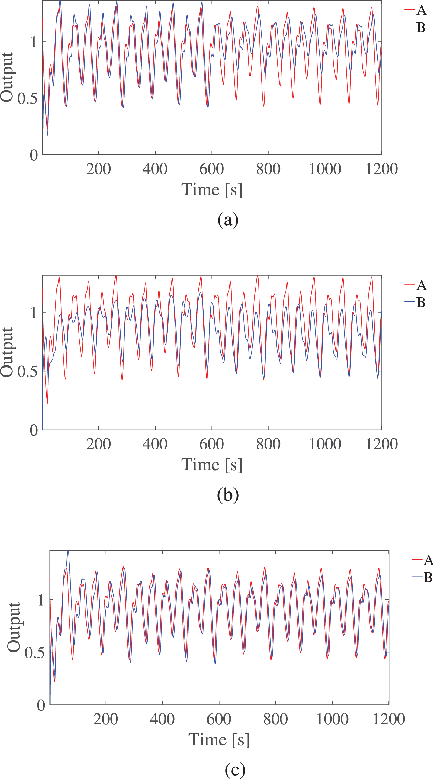
Modeling of MG time series. The subfigures: (a) LSTM, (b) fuzzy WN, and (c) fuzzy LSTM. “A” is the time series response and “B” is the network response.

4.2 Nonlinear system

We selected the benchmark problem proposed in [29] and [23] as the second example, this problem corresponds to a MIMO (multi-input-multi-output) nonlinear system in discrete time. As in the first example, a model generation for this system is required. The system is defined as: $\begin{matrix} y_{1} (k + 1) = \frac{0.5 y_{1} (k)}{1 + y_{2}^{2} (k) + u_{1} (k)} \\ y_{2} (k + 1) = \frac{0.5 y_{1} (k) y_{2} (k)}{1 + y_{2}^{2} (k) + u_{2} (k)} \end{matrix}$ (43) where y (k) = [y₁ (k) , y₂ (k)] ^T . We used different input signals for the training and the testing of (43). The training signals are $\begin{matrix} [c] c u_{1} (k) = 24.7 sin (\frac{2 π kT}{10}) + 0.5 cos (2 π kT) \\ u_{2} (k) = 24.5 sin (\frac{π kT}{10}) + 0.5 sin (π kT) \end{matrix}$ (44) and the testing signals are $\begin{matrix} [c] c u_{1} (k) = {\begin{matrix} [c] l If 0 < kT \leq 50, \\ u_{1} = 3.3 sin (\frac{2 π kT}{10}) + 0.1 cos (2 π kT) \\ If 50 + n_{u_{1}} < kT \leq 55 + n_{u_{1}}, u_{1} = 3.5 \\ If 55 + n_{u_{1}} < kT \leq 60 + n_{u_{1}}, u_{1} = - 3.5 \\ If 100 < kT, u_{1} = 3.6 cos (\frac{2 π kT}{10}) \end{matrix} \\ u_{2} (k) = {\begin{matrix} [c] l If 0 < kT \leq 50, \\ u_{2} = 3.5 sin (\frac{π kT}{10}) + 0.3 sin (π kT) \\ If 50 + n_{u_{2}} < kT \leq 55 + n_{u_{2}}, u_{2} = - 3.5 \\ If 55 + n_{u_{2}} < kT \leq 60 + n_{u_{2}}, u_{2} = 3.5 \\ If 100 < kT, u_{2} = 3.6 cos (\frac{2 π kT}{10}) \end{matrix} \end{matrix}$ (45)

with n_{u
₁} = n_{u
₂} = 10, 20, 30, 40.

Similar to the past example, the vector y (k) = [y₁ (k) , y₂ (k)] ^T was constructed by taking samples of the system with a sample period T = 0.01s, the input vector was defined as U_r (k) = [u₁ (k) , u₂ (k)]. To simulate perturbations, random values in [-0.5, 0.5] are added to U_r and y (k) in the training phase and random values in [-0.2, 0.2] are added to U_r and y (k) in the testing phase of the algorithms. While the. In this example, we used p = 18 fuzzy rules for the fuzzy systems (m = 2, κ = 3, l = 2), the dimensions of the NNs are defined from several tests with different sizes and choosing the smallest NNs that offers a good performance.

Fig. 4

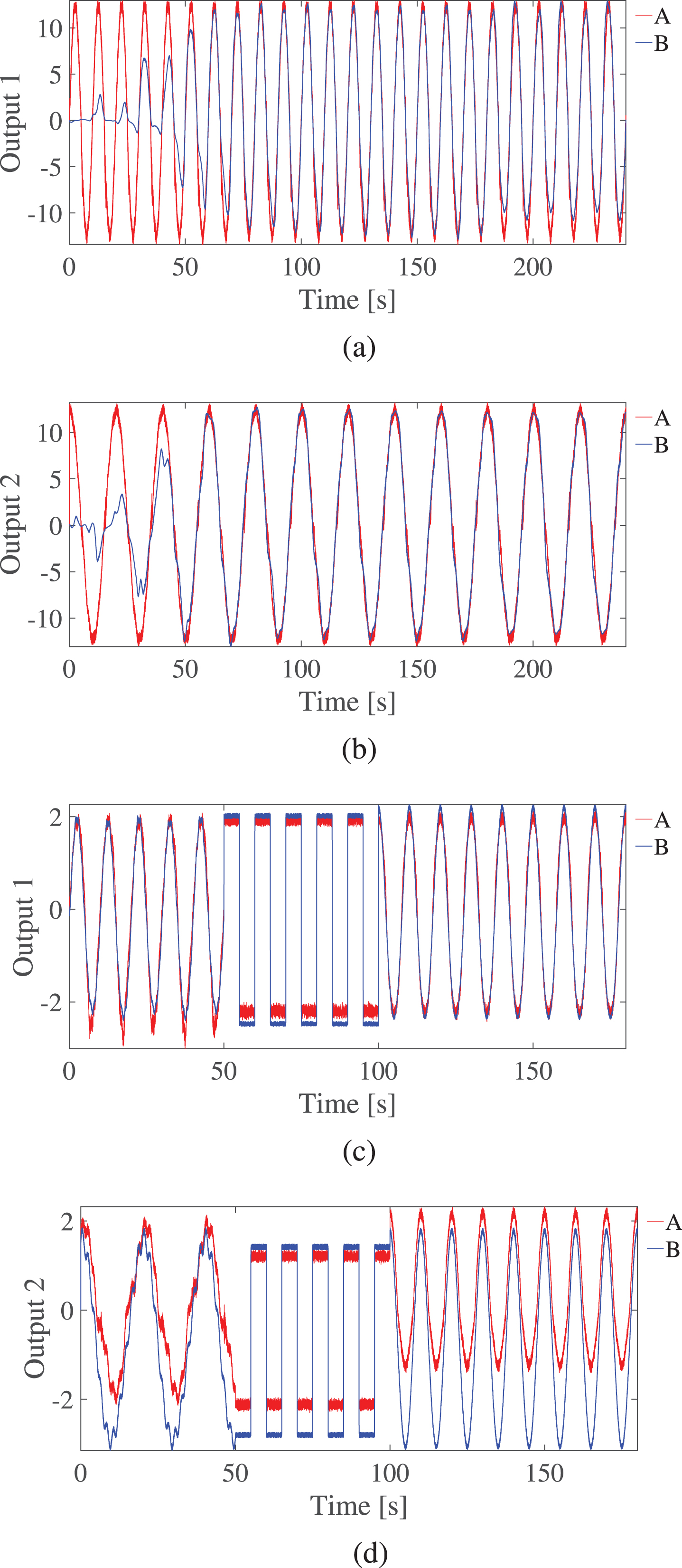
Nonlinear system modeling with “fuzzy WN”. The subfigures: (a) y₁ (k) in the training, (b) y₂ (k) in the training, (c) y₁ (k) in the testing, (d) y₂ (k) in the testing. “ A” is the system response and “B” is the model response.

Fig. 5

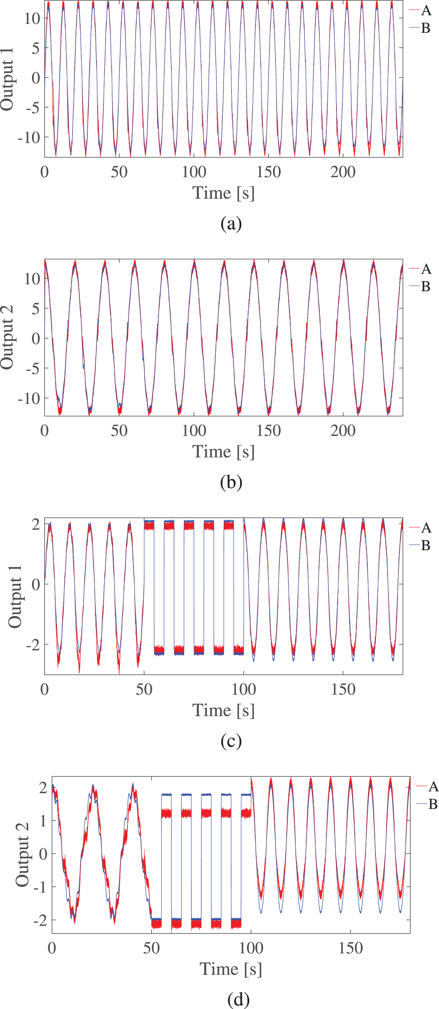
Nonlinear system modeling with “fuzzy LSTM”. The subfigures: (a) y₁ (k) in the training, (b) y₂ (k) in the training, (c) y₁ (k) in the testing, (d) y₂ (k) in the testing. “ A” is the system response and “B” is the model response.

We simulated the system in the following way: we train the algorithms to learn the system (43) with (44) during 180s, obtaining 18, 001 iterations for the training process, a testing is made immediately after the training with the same input signal during 60s (6,001 iterations). Also, a testing with a different input from the training (45) was made during 180s, obtaining 18, 001 iterations for this process.

In the Table 2 are shown the modeling errors, according to (18), obtained for each intelligent algorithm at the end of the training and testing phases. In this table, the NNs seem to have a better performance than the fuzzy systems, in the sense that this algorithms converges fast and offers a lower modeling error. Only our proposal has a similar (even slightly better) performance that the NNs.

Table 2

Modeling errors of the nonlinear system estimation (×10^-2)

Model	Training	Testing
		After training	Other input
KFRNN	52.56	57.95	17.95
LSTM	48.21	58.53	16.94
ANFIS 0	303.21	315.14	127.88
ANFIS 1	102.80	104.38	59.86
Fuzzy KFRNN	182.69	223.30	22.93
Fuzzy WN	1,382.32	1,070.40	48.20
Fuzzy LSTM	43.69	42.06	8.04

The Fig. 4 and 5 give the modeling processes of the “fuzzy WN” and the “fuzzy LSTM”. We show the “fuzzy WN” and the “fuzzy LSTM” because for this example all the other fuzzy systems had a similar performance that the “fuzzy WN”, and the other neural model had a similar performance the “fuzzy LSTM”. So, our proposal can generate an acceptable model for nonlinear systems with fast convergence, like a NN but offering a more complete approach, a gray box model instead of a black box model.

As shown in above figures and tables, the proposal model offers very good modelling results for the time series and the nonlinear system. Also it has better robustness and adaptability. It has been shown that our method has better testing results for multi-step prediction, or when some recent data are not available.

5 Conclusions

In order to obtain better approximation and fast training for TS models, we propose a novel fuzzy-neural network which applies the LSTM networks into the TS model. This model can be interpreted as more complete LSTM networks. Since the data for the model can be explained in the sense of fuzzy systems, the performances of both TS models and LSTM models are improved.

We also design a fast training method for this fuzzy LSTM network to overcome the training problem of the LSTM networks when they are applied in online cases. Stability analysis of the proposed algorithm is given. We use two examples to compare our model with the other intelligent algorithms, the results show that the new model is faster and has better performances than the other algorithms for nonlinear system identification. Our future work will be real world applications of the proposed fuzzy-neural network.

References

Blej

, Azizi

, Comparison of mamdani-type and sugeno-type fuzzy inference systems for fuzzy real time scheduling, International Journal of Applied Engineering Research 11(22) (2016), 11071–11075.

Jang

J.-S.

, Anfis: adaptive-network-based fuzzy inference system, IEEE Transactions on Systems Man and Cybernetics 23(3) (1993), 665–685.

Sremac

, Tanackov

, Kopic

, Radovic

, ANFIS model for determining the economic order quantity, Decision Making: Applications in Management and Engineering 1(2) (2018), 81–92.

Stojcic

, Atjepanovic

, Stjepanovic

, ANFIS model for the prediction of generated electricity of photovoltaic modules, Decision Making: Applications in Management and Engineering 2(1) (2019), 35–48.

Dong

, Wang

, Yang

G.-H.

, Output feedback fuzzy controller design with local nonlinear feedback laws for discretetime nonlinear systems, IEEE Transactions on Systems Man and Cybernetics, Part B (Cybernetics) 40(6) (2010), 144–41459.

Kabziski

, Kacerka

, Tsk fuzzy modeling with nonlinear consequences, in IFIP International Conference on Artificial Intelligence Applications and Innovations Springer (2014), pp. 498–507.

BenÃ-tez

J.M.

, Castro

J.L.

, Requena

, Are artificial neural networks black boxes? IEEE Transactions on Neural Networks 8(5) (1997), 1156–1164.

Babuka

, Verbruggen

, Neuro-fuzzy methods for nonlinear system identification, Annual Reviews in Control 27(1) (2003), 73–85.

Jin

, Sendhoff

, Extracting interpretable fuzzy rules from rbf networks, Neural Processing Letters 17(2) (2003), 149–164.

10.

Ganjefar

, Tofighi

, Single-hidden-layer fuzzy recurrent wavelet neural network: Applications to function approximation and system identification, Information Sciences 294 (2015), 269–285.

11.

Yu Jose de Jesus Rubio

, Recurrent neural networks training with stable bounding ellipsoid algorithm, IEEE Transactions on Neural Networks 20(6) (2009), 983–991.

12.

Chung

, Gulcehre

, Cho

, Bengio

, Empirical evaluation of gated recurrent neural networks on sequence modeling, arXiv preprint arXiv:1412.3555, (2014).

13.

Salehinejad

, Sankar

, Barfett

, Colak

, Valaee

, Recent advances in recurrent neural networks, arXiv preprint arXiv:1801.01078, (2017).

14.

Hochreiter

, Schmidhuber

, Long short-term memory, Neural Computation 9(8) (1997), 1735–1780.

15.

Ogunmolu

, Gu

, Jiang

, Gans

, Nonlinear systems identification using deep dynamic neural networks, arXiv preprint arXiv:1610.01439, (2016).

16.

Wang

, A new concept using lstm neural networks for dynamic system identification, in 2017 American Control Conference (ACC). IEEE, (2017), pp. 5324–5329.

17.

Nicola

, Fujimoto

, Oboe

, A lstm neural network applied to mobile robots path planning, in 2018 IEEE 16th International Conference on Industrial Informatics (INDIN). IEEE, (2018), pp. 349–354.

18.

Liu

, Zhou

, Li

, Attitude estimation of unmanned aerial vehicle based on lstm neural network, in 2018 International Joint Conference on Neural Networks (IJCNN). IEEE, (2018), pp. 1–6.

19.

Ergen

, Kozat

S.S.

, Effcient online learning algorithms based on lstm neural networks, IEEE Transactions on Neural Networks and Learning Systems 29(8) (2017), 3772–3783.

20.

Aviles

A.I.

, Alsaleh

S.M.

, Montseny

, Sobrevilla

, Casals

, A deep-neuro-fuzzy approach for estimating the interaction forces in robotic surgery, in 2016 IEEE International Conference on Fuzzy Systems (FUZZ-IEEE). IEEE, (2016), pp. 1113–1119.

21.

Sang

, Yang

, Liu

, Yun

, Jin

, A fuzzy neural network sliding mode controller for vibration suppression in robotically assisted minimally invasive surgery, The International Journal of Medical Robotics and Computer Assisted Surgery 12(4) (2016), 670–679.

22.

Sri

H.M.

, Rao

, Kammardi

P.K.

, Shekar

S.S.

, Kathavate

, Gowranga

, A smart adaptive lstm technique for electrical load forecasting at source, in 2017 2nd IEEE International Conference on Recent Trends in Electronics, Information & Communication Technology (RTEICT). IEEE, (2017), pp. 1717–1721.

23.

Sastry

, Santharam

, Unnikrishnan

, Memory neuron networks for identification and control of dynamical systems, IEEE Transactions on Neural Networks 5(2) (1994), 306–319.

24.

Chaudhary

, Patel

, Scholar

, A survey on backpropagation algorithm for neural networks, Int J Technol Res Eng 2(7) (2015).

25.

Jaeger

, Tutorial on training recurrent neural networks, covering BPPT, RTRL, EKF and the echo state network approach, GMD-Forschungszentrum Informationstechnik Bonn 5 (2002).

26.

Lipton

Z.C.

, Berkowitz

, Elkan

, A critical review of recurrent neural networks for sequence learning, arXiv preprint arXiv:1506.00019, (2015).

27.

, Nonlinear system identification using discrete-time recurrent neural networks with stable learning algorithms, Information Sciences 158(1) (2004), 131–147.

28.

Wang

L.X.

, Adaptive Fuzzy Systems and Control, Englewood Cliffs NJ: Prentice-Hall (1994).

29.

Narendra

K.S.

, Mukhopadhyay

, Adaptive Control Using Neural Networks and Approximate Models, IEEE Trans Neural Networks 8 (3) (1997), 475–485.

30.

, Li

, Fuzzy identification using fuzzy neural networks with stable learning algorithms, IEEE Transactions on Fuzzy Systems 12(3) (2004), 411–420.

31.

Shihabudheen

, Pillai

, Recent advances in neuro-fuzzy system: A survey, Knowledge Based Systems 152 (2018), 136–162.