Supervised electricity tariff prediction using random forest validated through user comfort and constraint for a home energy management scheme

Abstract

Day-ahead electricity tariff prediction is advantageous for both consumers and utilities. This article discusses the home energy management (HEM) scheme consisting of an electricity tariff predictor and appliance scheduler. The random forest (RF) technique predicts a short-term electricity tariff for the next 24 hours using the past three months of electricity tariff information. This predictor provides the tariff information to schedule the appliances at the most preferred time slot of a consumer with minimum electricity tariff, aiming high consumer comfort and low electricity bill for consumers. The proposed approach allows a user to be aware of their demand and their comfort. The proposed approach makes use of present-day (D) tariff and immediate previous 30 days (D-1, D-2, ... , D-30) of tariff information for training achieves minimum error values for next day electricity tariff prediction. The simulation results demonstrate the benefits of the RF approach for tariff prediction by comparing it with the support vector machine (SVM) and decision tree (DT) predicted tariffs against the actual tariff, provided by the utility day-ahead. The outcomes indicate that the RF produces the best results compared to SVM and DT predictions for performance metrics and end-user comfort.

Keywords

Day-ahead tariff decision tree home energy management random forest support vector machine

1 Introduction

Demand Response (DR) shifts the electricity demand from peak periods to off-peak periods, resulting in peak demand reduction [11, 26]. DR encourages users to modify their demand profiles according to the utility company incentives offered [37]. The user’s involvement through a priority-based incentive mechanism is motivated. The incentive mechanism utilizes the frequency of the participation of users in the DR program [21]. The primary motivation behind this is to achieve high-quality energy service with low energy costs. Under DR, pertinent information must be sent to the end-users by the utility, typically as an electrical tariff data. The electrical tariff increase may be ascribable to a rise in demand or buying power and redeeming it. Many researchers have modeled the residential DR under time-based pricing. The primary motivation is to minimize residential users’ electricity bills [1, 2].

Home energy management (HEM) systems in residential communities play a vital part under the DR strategy for the effective participation of end-users in response to the demand. The HEM system uses a scheduling algorithm developed to determine day-ahead appliance scheduling under hourly pricing and peak power-limiting [30]. Residential power utilization was scheduled based on electricity cost and users’ satisfaction of comfort [22]. The primary motivation for scheduling algorithms is to find the best time for appliances’ to be scheduled to cut the electricity bill.

The optimal decision of the HEM system towards appliances schedule is dependent on three key elements: (i) demand for energy, (ii) availability of energy, and (iii) tariff of electricity [9]. To make the optimal decisions, the HEM must have reliable predictors to have accurate predictions of the future considering the past historical data. The precise prediction of electricity tariff is necessary for residential consumers to participate in the DR program [8]. The electricity tariff represents the connexion between the energy supply and the demand, becomes one of the most significant elements of the power sector [27]. Thus, accurate electricity tariff prediction is necessary and relevant for balancing the energy generation by the utility and the energy consumption by the consumer. The electricity tariff prediction is too stochastic, which is not predictive every time with the required precision. The prediction depends upon several factors for example, the demand in energy varies based on the weather condition, the functionality of the energy resources, and daily activities of the consumer, which makes the electricity tariff frequently fluctuate [33]. Therefore, predicting high precision electricity tariff is not very easy.

The electricity tariff prediction has been a hot topic since introducing the dynamic tariffs for DR under the demand-side management umbrella [10, 13]. Prediction aims to fit the predicted data (obtained from past data) with the actual data as tightly as possible [12]. A day-ahead tariff prediction seems to be the best solution for the day-ahead electricity market [6], providing transparency to the utility to facilitate the generation side to balance demand and supply. The prediction can be a short term (ranges from an hour to a day), medium-term (ranges from a day to a month), long term (ranges from a month to a year), and very long term (ranges from a year to several years). Most researchers mostly prefer short-term prediction as it gives better results compared to other terms [25].

In literature, an observation is that the electricity hourly tariff has gotten attention for prediction in recent years [18]. It is observed that the artificial neural network (ANN) model is widely used for predicting electricity tariffs a day-ahead [16, 32]. Authors in [15] employed ANN to predict Ontario electricity tariffs. Authors in [29] projected a predictor consisting of an ANN and an evolutionary algorithm. However, the ANN encounters prediction errors during the testing stage due to the time-varying electricity tariff. A support vector machine (SVM) has been an alternative to the ANN for the data-driven technique suitable for specific scenarios [35]. SVM, also referred to as support vector regression, is used widely for predicting electricity tariffs as it falls into the category of the regression problem [7, 20]. However, there has been an increase in the overfitting problem [28].

The suitable machine learning technique cannot be preferred a priori. Perhaps a more straightforward substitute to ANN and SVM can be regression trees [14]. Nevertheless, regression trees are usually simpler and faster when trained. The authors in [31] tried a regression-tree-based model in the global energy forecasting competition and ranked first. The authors in [17] addressed the classification of short-term energy prices upon the decision tree method. They compared the result with ANN, and they found a decision tree produces a better result for the one-week ahead prediction time horizon. Authors in [4] proposed a random forest electricity prediction model to predict the CAISO market day-ahead. They considered very-short term, short term, long term, temporal, and geographic as features for error reduction towards electricity price prediction. Similarly, in [19] authors proposed a random forest for real-time price forecasting. The model uses three hours ago, one day ago, one week ago, and one month ago pricing information as features for forecasting. They compared the random forest results with an autoregressive moving average model (ARMA) and an ANN model and found that RF produces better prediction results.

Upon the existing literature, the proposed work focuses on predicting electricity tariffs (considering the time of day, day of the week, day of the month, week of the month, weekday/weekend, and immediate 30 days of electricity tariff data as the features) using random forest (RF) in comparison with SVM and decision tree (DT) towards end-user comforts for appliance scheduling at suitable time slots (high consumer comfort and reduced electricity bill of the consumer). The energy-demand differs for the time of the day, day of the week, day of the month, and the week of the month, directly proportional to the environmental conditions of wind, temperature, humidity, and seasons. This paper proposes the electricity tariff prediction algorithm for user comfort and utility constraint-based HEM. In this article, the scheduler follows a predictor to manage the energy within the residential home. The predictor forecasts the tariff closer to actual tariffs using the past tariff information (3 months). The scheduler plans the operation of the appliances during low tariff hours. The predictor and scheduler enable the user to be aware of their demand and comfort ahead of actual tariffs from the utility, creating flexibility for the consumer towards their appliance usage, thereby reducing the user discomforts (delay in appliances operation) in energy management.

The rest of the paper is structured as follows. Section II presents the architecture of the HEM scheme briefly. Section III is devoted to the mathematical formulation and the algorithms. Section IV elucidates the developed system’s simulation results, and finally, Section V provides the conclusion.

2 Supervised electricity tariff prediction

The predictor module predicts the hourly electricity tariff using past tariff data (3 months) before the day ahead real utility provided hourly tariff is available to the residential consumer. The inputs considered for the prediction techniques are the time of the day, day of the week, day of the month, week of the month, weekday or weekend, and past tariff data (90 sets of training data, each set of training data includes current day tariff (D) and immediate previous 30 days of tariff data (D-1, D-2, ... ., D-30)), as shown in Fig. 1.

Fig. 1

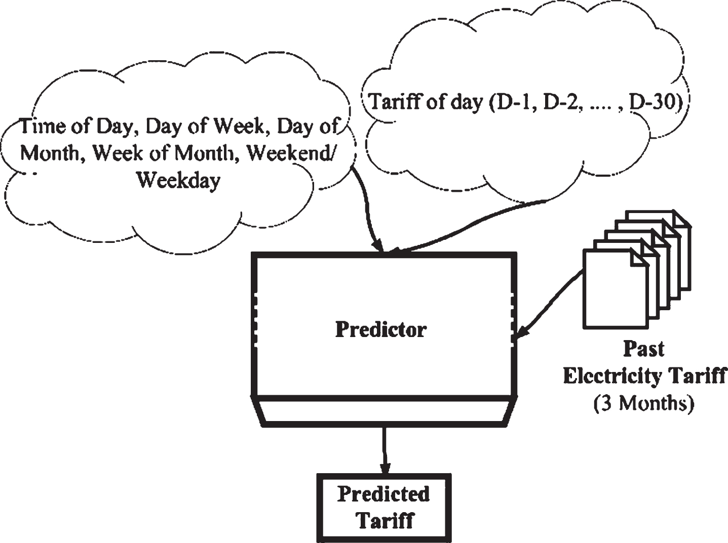
Flow process of the proposed HEM tariff predictor.

For electricity tariff prediction, the input parameters listed in the previous paragraph, from the utility provided past hourly tariff information of the year 2017/18 shown in Fig. 2 taken from ComEd Live Prices (cents converted to rupees) [5]. This data serves as input to the supervised learning algorithm that predicts hourly tariff information as part of the HEM. The parameters derived from hourly tariff data, used as input data variables for any day as part of the immediately previous 90 days of training dataset provided to learning algorithms for predicting the electricity tariff for a particular day, are listed in Table 1.

Fig. 2

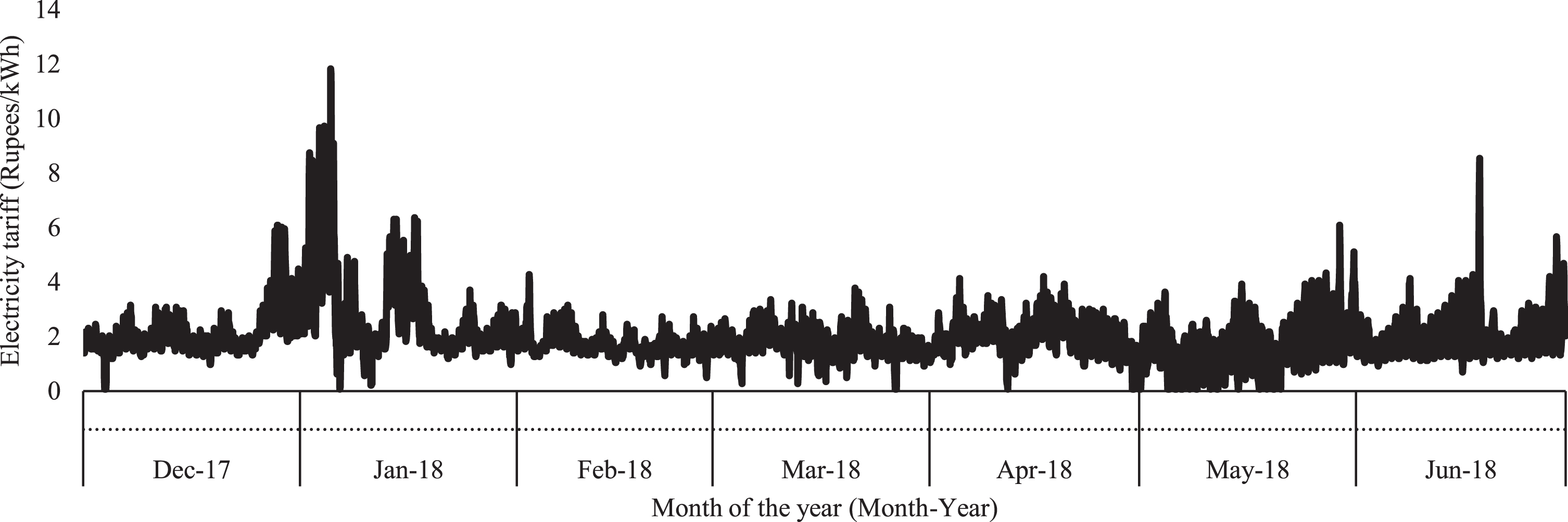
Electricity hourly tariff data considered for analysis.

Table 1

Input data variables derived from the hourly tariff data and used for electricity tariff prediction

Variables	Units
Time of day	Time ranges from 0 to 23
Day of week	Mon = 1, Tue = 2, Wed = 3, Thu = 4, Fri = 5, Sat = 6, Sun = 7
Day of month	Day ranges from 1 to 31
Week of month	Week ranges from 1 to 5
Weekday or Weekend	Weekday = 1 or Weekend = 2
Tariff of the Current Day (D)	Rs/kWh
Tariff of the Previous Day for D (D-1)	Rs/kWh
Tariff of the Previous Day for D-1 (D-2)	Rs/kWh
·	·
·	·
Tariff of the Previous Day for D-29 (D-30)	Rs/kWh

The formulation of the tariff prediction is done and analyzed based on three prediction techniques, namely SVM, DT, and RF (as discussed in algorithm 1).

2.1) Support Vector Machine (SVM):

SVM is a supervised machine learning approach that constructs the hyperplane in n-dimensional space [36]. SVM uses the concept of support vectors to construct the hyper-plane. SVM supports both regression and classification analysis, where the regression function is enabled by support vector regression (SVR), while the support vector classifier enables the classification function. The SVR maps the high dimensional variables with the input training data. The SVR function is shown in Equation 1. $F (a) = \min \frac{1}{2} ∥ a ∥^{2} such that | y_{m} - (a^{T} x_{m} + b) | ⩽ ɛ$ (1)

where,

∥a∥ –is the Euclidean Norm.

x_m –is the training sample.

y_m –is the target value.

a^T x_m + b –is the prediction for the training sample.

ɛ –is the threshold.

Without knowing the mapping transformation function, the kernel methods are introduced in SVR to solve the mapping function by computing the dot product between two mappings that transforms into the variable space. Kernel functions, including the linear kernel, poly kernel, radial basis function kernel, sigmoid kernel, and the pre-computed kernel, are used for computing the mapping function. The commonly used kernel function for SVM is the radial basis function (RBF) [34]. The RBF is calculated, as shown in Equation 2. $RBF = e^{(- γ ∥ x_{m} - x_{n} ∥^{2})}$ (2) where,

x_m –is the training sample

x_n –is the testing sample

given that, $γ = \frac{1}{Feature Count}$

Algorithm 1: Pseudo Code for Predicting Electricity Tariff
Training data: Time of day, day of week, day of month, week of month, weekday or weekend, past tariffs (D-1, D-2, ... , D-30).
Target data: Tariff of the day (D).
Predicted data: Electricity tariff of the next day.
Begin:
1. Read the data from comma-separated value (CSV) file in order as the time of day, day of the week, day of the month,
week of the month, weekday or weekend, past tariffs (D-1, D-2, ... , D-30), and tariff of the day (D).
2. Visualize read data as input featured data (time of day, day of the week, day of the month, week of the month, weekday
or weekend), past tariffs (D-1, D-2, ... , D-30), and tariff of t day (D).
3. Segregating input featured data as x and target data as y.
4. Build a supervised learning algorithm:
If (SVR = = TRUE)
(a) Model the predictor using support vector regression with the following parameters:
Kernel = Radial basis function; Cache size = 200; Maximum iteration =&thinsp-1; Tolerance = 0.001; epsilon = 0.1
If (DT = = TRUE)
(b) Build a decision tree predictor using decision tree regression with the following parameters:
Criterion = Mean Absolute Error; Minimum Sample Leaf = 1; Minimum Sample Split = 2; Random State = None; Splitter = ‘Best’
If (RF = = TRUE)
(c) Build random forest predictor using random forest regression with the following parameters:
Bootstrap = ‘True’; Criterion = Mean Absolute Error; Maximum Feature = ‘Auto’; Minimum Sample Leaf = 1;
Minimum Sample Split = 2; Number of estimators = 10; Random State = None
5. Do model fitting
6. Predict the tariff for the next day using time of day, day of the week, day of month, week of month, weekday or weekend, past tariff.

2.2) Decision Tree (DT):

DT is a supervised machine learning algorithm representing a flow chart tree structure used for classification and regression problems [24]. In this learning algorithm, during training, the data is segregated into different nodes of the tree. The DT starts with the root node, where the input data are categorized into several groups [38]. There are two main entities in DT; they are decision nodes (points where data splits) and leaf nodes (which makes decisions). Once the decision node is arrived, based on the rule selected, the decision node is split into two child nodes. Further, these child nodes undergo the recursive procedure as a decision node until it reaches some stopping criteria.

For decision tree regressors, there is a need for an impurity metric suitable for continuous variables. Therefore, the impurity measure using the mean absolute error (MAE_DT) of the child node is defined using Equation 3. The variables with the most considerable mean absolute error reduction is chosen as the decision node to select the best split. ${MAE}_{DT} = \frac{1}{N_{n}} \sum_{m \in S_{n}} | y_{m} - {\hat{y}}_{n} |$ (3)

where,

N_n–is the number of training samples at node n.

S_n–is the training subset at node n.

y_m- is the target value

${\hat{y}}_{n}$ –is the mean of target value given as, ${\hat{y}}_{n} = \frac{1}{N_{n}} \sum_{m \in S_{n}} y_{m}$ (4)

2.3) Random Forest (RF):

RF is a collaborative learning method consisting of more than one DT for decision-making and regression problems [23]. DT can be updated incrementally, whereas RF cannot. Hence, in RF, all training data are likely to be available in advance. RF utilizes bootstrapping (choosing samples from the training set with replacement) and bagging (selection of values arbitrarily from the training values) principles. For any given new value, the prediction is done using either previously trained RF or retrain a whole new RF that includes both old and new data.

The functioning of random forest is as follows: Consider a dataset S., consisting of X rows data and Y. count of features. A few sets of rows x ∈ X. and few features y ∈ Y are selected randomly with replacement [3]. The randomly selected samples are feed to the decision tree. Similarly, multiple decision trees (here, 10 decision trees, are built as we have taken estimators equal to 10) are constructed for several combinations of randomly selected samples. Finally, train all the decision tree and for each decision tree obtain a predicted result. Now, the predicted values of all sample datasets are aggregated, and the predicted values are considered to be the most voted values for classification and the mean for the regression problems.

2.4) Performance Metrics Assessment:

Three months of electricity tariff data are used, with all three techniques (SVM, DT, and RF), and for the next day hourly tariff prediction. To evaluate the performance metrics of the predictor, three scenarios, are taken into consideration as follows,

Scenario 1: considers January-March Tariff data, thereby predicting the tariff forthe first day of April.

Scenario 2: considers February-April Tariff data, thereby predicting the tariff forthe first day of May.

Scenario 3: considers March-May Tariff data, thereby predicting the tariff forthe first day of June.

Figure 3(a) and 3(b) show the “scenario 1” as mentioned above, with and without considering D-1, D-2, ... , D-30 as input for training, respectively. From Fig. 3(a) and 3(b), it is observed that Fig. 3(b) depicts very close prediction from hour 1 to hour 24 (considering D, D-1, D-2, ... , D-30 tariff data). Similarly, from Figs. 4 and 5, it is observed that Figs. 4(b) and 5(b) shows close prediction from hour 1 to 24. However, there exists some error concerning the actual tariff (AT). An observation is that RF predicted tariff values follow the gesture of AT closely.

Fig. 3

Comparison between AT and predicted tariff (using SVM, DT, and RF) for 1st April 2018.

Fig. 4

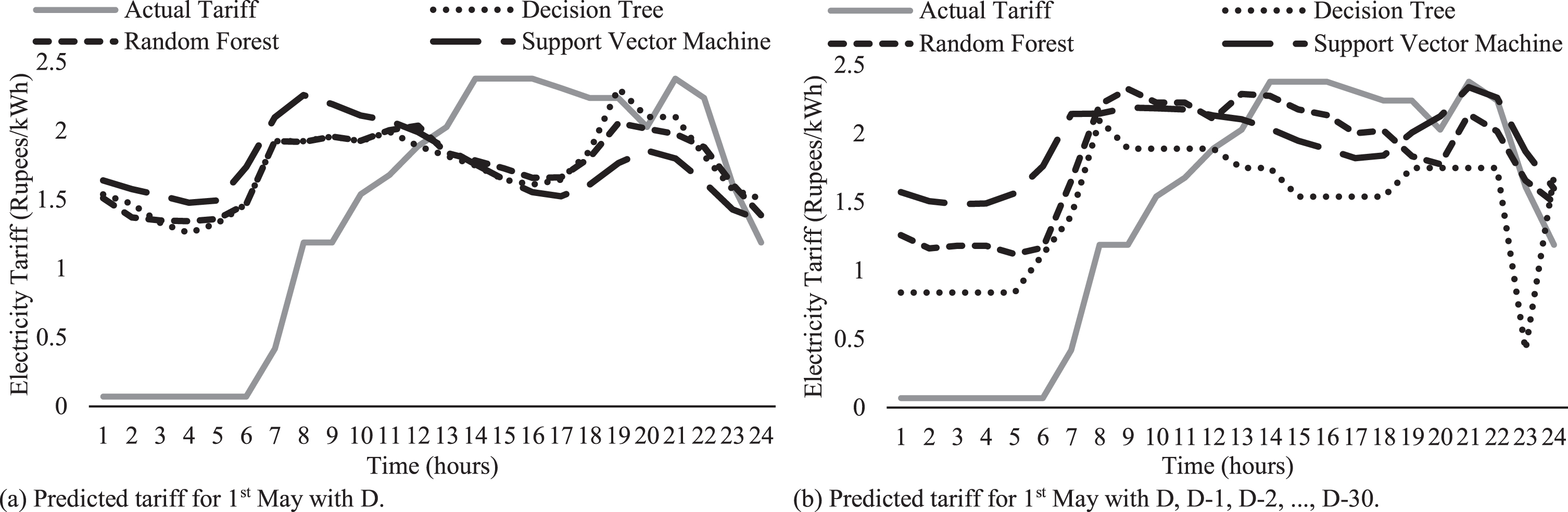
Comparison between AT and predicted tariff (using SVM, DT, and RF) for 1st May 2018.

Fig. 5

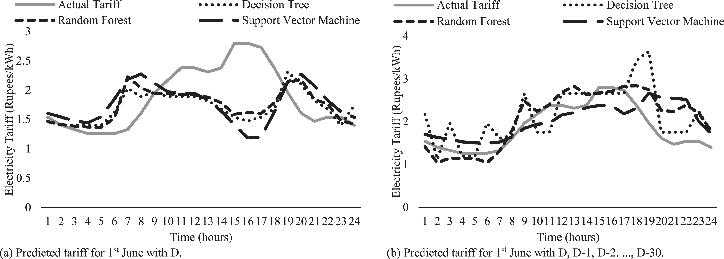
Comparison between AT and predicted tariff (using SVM, DT, and RF) for 1st June 2018.

The predicted values are assessed through performance metrics like Mean Absolute Error (MAE), Mean Square Error (MSE), Root Mean Square Error (RMSE), and Mean Average Percentage Error (MAPE), obtained from Eqs. 5, 6, 7, and 8, and the outcomes, are listed in Table 2.

Table 2

Performance Metrics of SVM, DT, and RF for predicting electricity tariff through MAE, MSE, RMSE, MAPE

	Metrics	MAE			MSE			RMSE			MAPE
	Techniques	SVM	DT	RF	SVM	DT	RF	SVM	DT	RF	SVM	DT	RF
1st April	Tariff (D)	0.299	0.150	0.149	0.133	0.034	0.034	0.365	0.185	0.183	0.223	0.111	0.113
	Tariff (D, D-1, D-2,..., D-30)	0.244	0.111	0.104	0.100	0.021	0.016	0.317	0.144	0.125	0.197	0.076	0.071
1st May	Tariff (D)	0.825	0.678	0.677	0.950	0.702	0.693	0.975	0.838	0.833	5.759	5.058	5.062
	Tariff (D, D-1, D-2,..., D-30)	0.722	0.653	0.596	0.846	0.504	0.535	0.920	0.710	0.731	5.677	3.241	4.255
1st June	Tariff (D)	0.525	0.438	0.403	0.469	0.331	0.297	0.685	0.575	0.545	0.267	0.215	0.199
	Tariff (D, D-1, D-2,..., D-30)	0.363	0.423	0.328	0.215	0.313	0.173	0.464	0.560	0.416	0.213	0.239	0.192

$MAE = \frac{1}{24} \sum_{h = 1}^{24} | actual tariff - predicted tariff |$ (5) $MSE = \frac{1}{24} \sum_{h = 1}^{24} {(actual tariff - predicted tariff)}^{2}$ (6) $RMSE = \sqrt{\frac{1}{24} \sum_{h = 1}^{24} {(actual tariff - predicted tariff)}^{2}}$ (7) $MAPE = [\frac{1}{24} \sum_{h = 1}^{24} (| \frac{actual tariff - predicted tariff}{actual tariff} |)] * 100$ (8)

Table 2 infers the reduction in error values upon considering the tariff of the day (D, D-1, D-2,...., D-30) for prediction in comparison with the tariff of the day (D).

3 System model of home energy management scheme

The proposed energy management scheme takes into the assumption that every home has both schedulable and non-schedulable appliances. The non-schedulable appliances operate at the user-defined hour of the day and the schedulable appliances during the hours defined through a scheduler.

The scheduler considers the concept of appliance accommodation window (AAW) and soft-constraints (SC), as shown in Fig. 6. The AAW contains a range of time slots assigned for each schedulable appliance by the users. The SC is the maximum power consumption restriction provided by the utility (based on the non-schedulable load of a residential home) to maintain a power demand peaks. The scheduler module receives predicted hourly tariff information from the predictor, maximum power constraint from the utility, and AAW (for each schedulable appliance) as inputs from the user. Upon receiving the data, the scheduler schedules the appliance during the low tariff period within an AAW and SC without compromising user comforts.

Fig. 6

Flow process of the proposed HEM appliance scheduler.

Algorithm 2: Pseudocode for Scheduling Appliances
Input: Appliance demand, AAW, Predicted Electricity Tariff, and Hourly Soft-Constraint.
Output: Appliance Schedule pattern.
Begin:
1. Initialize SC_h = G_h, d_r = 0;
2. For each appliance a ∈ NA
3. For each hour h between 1 and 24 that lies within AAW
4. IfG_h ⩾ d_a// Check whether grid power at an hour h is sufficient to meet the demand
5. Then Schedule appliance a during that hour h;
6. G_h = G_h - d_a// Update left out grid power as available power for the next iteration
7. d_T = d_r + d_a// Update total demand d_T schedule till now
8. Go to step 3 for the next appliance a
9. The schedule for non-schedulable appliances is obtained.
10. For each appliance a ∈ SA
11. For each turn of appliance operation
12. For each hourh between 1 and 24 that lies within AAW
13. If ((G_h ⩾ d_a) and (d_r + d_a ⩽ SC_h)) // Check whether grid power at an hourh is sufficient to meet the demand within the threshold
14. And also, tariff during that specific hour is minimum in comparison with other tariffs within AAW
15. Then Schedule appliance a during that hour h ;
16. G_h = G_h - d_a// Update left out grid power as available power for the next iteration
17. d_T = d_T + d_a// Update total demand d_T schedule till now
18. Go to either step 12 for the next turn or step 11 for the next appliance a
19. The schedule for schedulable appliances is obtained.

HEM’s primary role is to predict the electricity tariff closer to the actual tariff and regulate power demand within the constraint and comfort. The scheduler calculates the respective home’s hourly power consumption and checks whether the consumption exceeds the constraint. If so, then the schedulable appliances are shifted to the next lowest tariff slots, confirming that the power consumption is within the constraint. The next slot is also chosen within the AAW for any particular appliance to remain uncompromised with the user comfort.

The scheduler schedules the appliances so that it minimizes the users’ electricity bills without affecting their comfort. An assumption in this article is that the non-schedulable appliances operate during the hours that belong to AAW. In contrast, schedulable appliances operate during a reasonable low tariff hour that belongs to AAW, as discussed in algorithm 2 in subsequent Section 3.1.

3.1) Mathematical framework for appliance scheduling:

We assume a set of appliances, classified into two broad categories of sets, based on their demand-type schedulable and non- schedulable. These appliances are scheduled to their defined time slots or to an appropriate time slot based on their type. The schedulable appliances SA get schedule by shifting their demand to an appropriate time slot, whereas non- schedulable appliances NA operate at their respective defined time slots without shifting.

For an appliance a, the assumption is that the demand remains constant during its operation. When the rating of an appliance is R_a, then the demand d_a per its operational length n_a is as listed in Equation 9. $d_{a} = \frac{R_{a}}{n} * n_{a}$ (9)

where,

R_a - Rating of an appliance in terms of kW per hour.

n - number of minutes in an hour (Typically 60).

n_a - Total number of minutes an appliance operates.

In this article, we assumed that there is a seamless grid power every hour of the day G_h, and its hourly tariff information, from the utility, day-ahead. The scheduler utilizes low tariff hours to reduce EB if demand management is with grid power. However, this can cause demand peaks not appropriate for the grid. Therefore, the article considers an hourly soft-constraint SC_h on power drawn from the grid to reduce such peaks.

4 Results and discussion

To demonstrate the effectiveness of our proposed approach, three homes with layouts in Table 3, with a different set of appliances listed in Table 4, with different usage patterns listed in Table 5, are considered.

Table 3
List of rooms considered for analysis in each home

Room Name Home 1 Home 2 Home 3

Living Room √ √ √

Bed Room 1 √ √ √

Bed Room 2 x x √

Kitchen √ √ √

Bath Room √ √ √

Room Name	Home 1	Home 2	Home 3
Living Room	√	√	√
Bed Room 1	√	√	√
Bed Room 2	x	x	√
Kitchen	√	√	√
Bath Room	√	√	√

√ - Available, x - Not Available.

Table 4

List of household appliances and their rating used for analysis in each home

Appliance Name	Power Rating (kWh)	Home 1	Home 2	Home 3
Television-I	0.2	x	√	√
CFL Lamp	0.01	√	√	√
Computer	0.1	√	x	x
Computer with Printer	0.25	x	√	√
Exhaust Fan	0.04	x	√	√
Fan	06	√	√	√
Mixer	0	√	√	√
Radio	0.04	√	√	√
Refrigerator 165 L	08	√	x	x
Refrigerator 210 L	0.25	x	√	√
Television-II	x	√
Toaster	0.75	x	x	√
Tube Light	0.02	√	√	√
AC 1 Ton	1.5	√	x	x
AC 1.5 Ton	2.25	x	√	√
Electric Iron	0.75	√	√	√
Microwave Oven	1	√	√	√
Motor Pump	0.37	√	√	√
Washing Machine	0.55	√	x	x
Washing Machine with Dryer	1.5	x	√	√
Water Heater - Geyser	1	√	√	√

√ - Used, x - Not Used.

Table 5

Preferred time slots for each schedulable appliance used in each home

Schedulable Appliances	Home 1	Home 2	Home 3
	Appliance Operation Time (Hour)	Appliance Operation Time (Hour)	Appliance Operation Time (Hour)
Electric Iron	Operation 1:7–9	Operation 1:6–8	Operation 1: 7–9
			Operation 2: 19–22
Microwave Oven	Operation 1: 12-13	Operation 1: 11-12	Operation 1: 12-13
	Operation 2: 18–20	Operation 2: 18-19	Operation 2: 19-20
Motor Pump	Operation 1: 16–19	Operation 1: 5–7	Operation 1: 5–7
			Operation 2: 17–19
Washing Machine	Operation 1: 10–13	x	x
			Operation 2: 16–19
Washing Machine with Dryer	x	Operation 1: 9–12	Operation 1: 9–14
		Operation 2: 18–23	Operation 2: 16–22
Water Heater-Geyser	Operation 1: 6–8	Operation 1: 6-7	Operation 1: 5–7
	Operation 2: 18-19	Operation 2: 20-21	Operation 2: 20-21

x - Not Used.

Table 6, Table 7, and Table 8 list the scheduled hour of an appliance using Ad-hoc time slots chosen by the user, and the scheduler’s time slots concerning the AT, SVM, DT, and RF tariffs, considering scenarios as discussed in section 2.4. In comparison with an AT-based scheduling hour for all scenarios, the maximum waiting time for an appliance operating range between,

Table 6

Appliance scheduled time slot (hours) w. r. t. Ad-hoc, AT, SVM, DT, and RF considering scenario 1

Appliances	Home 1					Home 2					Home 3
	Ad-hoc	AT	SVM	DT	RF	Ad-hoc	AT	SVM	DT	RF	Ad-hoc	AT	SVM	DT	RF
Electric Iron S1	7	7	7	7	7	7	6	7	7	6	8	7	7	7	7
Electric Iron S2	x	x	x	x	x	x	x	x	x	x	19	19	19	19	19
Microwave Oven S1	12	13	13	12	13	12	11	11	11	11	12	13	13	12	13
Microwave Oven S2	19	18	18	18	19	19	18	18	18	19	19	19	19	19	19
Motor Pump S1	18	16	18	17	19	6	5	7	7	5	6	5	7	7	5
Motor Pump S2	x	x	x	x	x	x	x	x	x	x	18	17	18	17	19
Washing Machine S1	10	10	10	10	10	x	x	x	x	x	x	x	x	x	x
Washing Machine S2	18	16	18	17	19	x	x	x	x	x	x	x	x	x	x
Washing Machine with Dryer S1	x	x	x	x	x	10	9	10	9	9	10	9	14	14	14
Washing Machine with Dryer S2	x	x	x	x	x	18	18	18	18	19	18	16	18	17	18
Water Heater - Geyser S1	6	6	7	7	6	7	7	7	7	7	6	5	7	7	5
Water Heater - Geyser S2	19	18	19	18	18	21	19	19	19	21	21	20	20	20	21
Ad-hoc: time slot preferred by the user unaware of electricity tariff
AT: time slot chosen by the scheduler on the reception of electricity tariff from the utility
SVM: time slot chosen by the scheduler concerning support vector machine predicted electricity tariff
DT: time slot chosen by the scheduler concerning decision tree predicted electricity tariff
RF: time slot chosen by the scheduler concerning random forest predicted electricity tariff

x - Not Available.

Table 7

Appliance scheduled time slot (hours) w. r. t. Ad-hoc, AT, SVM, DT, and RF considering scenario 2

Appliances	Home 1					Home 2					Home 3
	Ad-hoc	AT	SVM	DT	RF	Ad-hoc	AT	SVM	DT	RF	Ad-hoc	AT	SVM	DT	RF
Electric Iron S1	7	7	7	7	7	7	6	6	6	6	8	7	7	7	7
Electric Iron S2	x	x	x	x	x	x	x	x	x	x	19	20	19	19	20
Microwave Oven S1	12	12	13	13	12	12	11	12	11	12	12	12	13	13	12
Microwave Oven S2	19	18	18	18	19	19	18	18	18	19	19	20	19	19	20
Motor Pump S1	18	18	17	16	19	6	5	5	5	5	6	5	5	5	5
Motor Pump S2	x	x	x	x	x	x	x	x	x	x	18	18	17	17	19
Washing Machine S1	10	10	12	10	12	x	x	x	x	x	x	x	x	x	x
Washing Machine S2	18	18	17	16	19	x	x	x	x	x	x	x	x	x	x
Washing Machine with Dryer S1	x	x	x	x	x	10	9	12	9	12	10	9	14	14	12
Washing Machine with Dryer S2	x	x	x	x	x	18	18	18	18	19	18	20	17	16	20
Water Heater - Geyser S1	6	6	6	6	6	7	7	7	7	7	6	5	5	5	5
Water Heater - Geyser S2	19	19	18	18	18	21	19	19	19	21	21	21	20	20	21

x - Not Available.

Table 8

Appliance scheduled time slot (hours) w. r. t. Ad-hoc, AT, SVM, DT, and RF considering scenario 3

Appliances	Home 1					Home 2					Home 3
	Ad-hoc	AT	SVM	DT	RF	Ad-hoc	AT	SVM	DT	RF	Ad-hoc	AT	SVM	DT	RF
Electric Iron S1	7	7	7	7	7	7	6	6	7	6	8	7	7	7	7
Electric Iron S2	x	x	x	x	x	x	x	x	x	x	19	21	22	20	21
Microwave Oven S1	12	13	12	12	12	12	11	11	11	11	12	13	12	12	12
Microwave Oven S2	19	19	18	18	19	19	19	18	18	19	19	20	20	20	20
Motor Pump S1	18	19	17	16	16	6	5	6	5	6	6	5	6	5	6
Motor Pump S2	x	x	x	x	x	x	x	x	x	x	18	19	17	17	19
Washing Machine S1	10	10	10	10	10	x	x	x	x	x	x	x	x	x	x
Washing Machine S2	18	19	17	16	16	x	x	x	x	x	x	x	x	x	x
Washing Machine with Dryer S1	x	x	x	x	x	10	9	9	10	10	10	9	9	10	10
Washing Machine with Dryer S2	x	x	x	x	x	18	19	18	18	19	18	22	17	20	20
Water Heater - Geyser S1	6	6	6	7	6	7	7	7	7	7	6	5	6	5	6
Water Heater - Geyser S2	19	18	18	18	19	21	21	21	21	21	21	21	21	21	21

x - Not Available.

Scenario one: 0 hours to 5 hours in SVM, DT, and RF, techniques.

Scenario two: 0 hour to 5 hours for SVM, DT (higher than RF waiting time that ranges between 0 to 3 hours).

Scenario three: 0 and 5 for SVM, (higher than both DT and RF waiting time that ranges between 0 to 3 hours).

Also, the average waiting time concerning the RF is fair enough for user satisfaction compared to SVM and DT for home 1, home 2, and home 3.

Table 9, Table 10, and Table 11 list user satisfaction percentage for each appliance using SVM, DT, and RF predicted tariff concerning the AT. The schedulable appliances scheduled time slot concerning predicted electricity tariff is the period at which appliances are schedule initially. Any deviation in that schedule concerning the actual electricity tariff affects user satisfaction (User_Sat.) calculated using Equation 10. For all scenarios, the average rate of user satisfaction for RF seems to be comparatively high (97.5%) when compared to DT (97%) and SVM (96.5%). Therefore, towards end-user preferences on the prediction scheme, RF seems to provide more satisfaction to the user.

${User}_{Sat} (%) = \frac{(T_{d} - | {STS}_{AT} - {STS}_{PT} |)}{T_{d}} * 100$ (10)

where,

T_d - Total time slots in a day (Typically 24, each slot of one-hour duration).

STS_AT - scheduled time slot for each schedulable appliance concerning actual electricity tariff from utility.

STS_PT –scheduled time slot for each schedulable appliance concerning predicted electricity tariff (SVM, DT, RF).

Table 9

User satisfaction in percentage (%) using SVM, DT, and RF w. r. t. AT considering scenario 1

Appliance	Home 1			Home 2			Home 3
	SVM_US	DT_US	RF_US	SVM_US	DT_US	RF_US	SVM_US	DT_US	RF_US
Electric Iron S1	100	100	100	95.83	95.83	100	100	100	100
Electric Iron S2	x	x	x	x	x	x	100	100	100
Microwave Oven S1	100	95.83	100	100	100	100	100	95.83	100
Microwave Oven S2	100	100	95.83	100	100	95.83	100	100	100
Motor Pump S1	91.67	95.83	87.5	91.67	91.67	100	91.67	91.67	100
Motor Pump S2	x	x	x	x	x	x	95.83	100	91.67
Washing Machine S1	100	100	100	x	x	x	x	x	x
Washing Machine S2	91.67	95.83	87.5	x	x	x	x	x	x
Washing Machine with Dryer S1	x	x	x	95.83	100	100	79.17	79.17	79.17
Washing Machine with Dryer S2	x	x	x	100	100	95.83	91.67	95.83	91.67
Water Heater - Geyser S1	95.83	95.83	100	100	100	100	91.67	91.67	100
Water Heater - Geyser S2	95.83	100	100	100	100	91.67	100	100	95.83
Average Percentage of User Satisfaction	96.875	97.915	96.35375	97.91625	98.4375	97.91625	95.001	95.417	95.834
SVM_US: Satisfaction percentage of the user using support vector machine predicted electricity tariff concerning AT
DT_US: Satisfaction percentage of the user using decision tree predicted electricity tariff concerning AT
RF_US: Satisfaction percentage of the user using random forest predicted electricity tariff concerning AT

x - Not Available.

Table 10

User satisfaction in percentage (%) using SVM, DT, and RF w. r. t. AT considering scenario 2

Appliance	Home 1			Home 2			Home 3
	SVM_US	DT_US	RF_US	SVM_US	DT_US	RF_US	SVM_US	DT_US	RF_US
Electric Iron S1	100	100	100	100	100	100	100	100	100
Electric Iron S2	x	x	x	x	x	x	95.83	95.83	100
Microwave Oven S1	95.83	95.83	100	95.83	100	95.83	95.83	95.83	100
Microwave Oven S2	100	100	95.83	100	100	95.83	95.83	95.83	100
Motor Pump S1	95.83	91.67	95.83	100	100	100	100	100	100
Motor Pump S2	x	x	x	x	x	x	95.83	95.83	95.83
Washing Machine S1	91.67	100	91.67	x	x	x	x	x	x
Washing Machine S2	95.83	91.67	95.83	x	x	x	x	x	x
Washing Machine with Dryer S1	x	x	x	87.5	100	87.5	79.17	79.17	87.5
Washing Machine with Dryer S2	x	x	x	100	100	95.83	87.5	83.33	100
Water Heater - Geyser S1	100	100	100	100	100	100	100	100	100
Water Heater - Geyser S2	95.83	95.83	95.83	100	100	91.67	95.83	95.83	100
Average Percentage of User Satisfaction	96.87375	96.875	96.87375	97.91625	100	95.8325	94.582	94.165	98.333

x - Not Available.

Table 11

User satisfaction in percentage (%) using SVM, DT, and RF w. r. t. AT considering scenario 3

Appliance	Home 1			Home 2			Home 3
	SVM_US	DT_US	RF_US	SVM_US	DT_US	RF_US	SVM_US	DT_US	RF_US
Electric Iron S1	100	100	100	100	95.83	100	100	100	100
Electric Iron S2	x	x	x	x	x	x	95.83	95.83	100
Microwave Oven S1	95.83	95.83	95.83	100	100	100	95.83	95.83	95.83
Microwave Oven S2	95.83	95.83	100	95.83	95.83	100	100	100	100
Motor Pump S1	91.67	87.5	87.5	95.83	100	95.83	95.83	100	95.83
Motor Pump S2	x	x	x	x	x	x	91.67	91.67	100
Washing Machine S1	100	100	100	x	x	x	x	x	x
Washing Machine S2	91.67	87.5	87.5	x	x	x	x	x	x
Washing Machine with Dryer S1	x	x	x	100	95.83	95.83	100	95.83	95.83
Washing Machine with Dryer S2	x	x	x	95.83	95.83	100	79.17	91.67	91.67
Water Heater - Geyser S1	100	95.83	100	100	100	100	95.83	100	95.83
Water Heater - Geyser S2	100	100	95.83	100	100	100	100	100	100
Average Percentage of User Satisfaction	96.875	95.31125	95.8325	98.43625	97.915	98.9575	95.416	97.083	97.499

x - Not Available.

5 Conclusion

This paper focused on day-ahead electricity tariff prediction using an SVM, DT, and RF approaches for the HEM scheme. The set of appliances (non-schedulable and schedulable), an electricity tariff predictor, and appliance scheduler are considered part of the HEM scheme in each home. The three houses with a different set of appliances and their different styles of consumption patterns help in demonstrating the proposed approach. An observation during simulations is that the RF electricity tariff prediction with the next 30 days of electricity tariff data as the features produced the best prediction towards the actual electricity pricing compared to the SVM and DT concerning the performance metrics. The simulation results indicate that the developed algorithm achieves higher user comfort (97.5%) during appliance scheduling while performing energy management.

Conflict of interest

The authors declare that they have no conflict of interest.

References

Anees

and Chen

Y.P.P.

, True real time pricing and combined power scheduling of electric appliances in residential energy management system, Applied Energy 165(1) (2016), 592–600.

Barbato

, Capone

, Carello

, et al., A framework for home energy management and its experimental validation, Energy Efficiency 7(6) (2014), 1013–1052.

Lahouar

and Ben Hadj Slama

, Day-ahead load forecast using random forest and expert input selection, Energy Conversion and Management 103 (2015), 1040–1051.

Sadeghi-Mobarakeh

, Kohansal

, Papalexakis

E.E.

and Mohsenian-Rad

, Data mining based on random forest model to predict the California ISO day-ahead market prices, 2017 IEEE Power & Energy Society Innovative Smart Grid Technologies Conference (ISGT), Washington, DC, (2017), 1–5.

ComEd’s hourly pricing program, (2019), https://hourlypricing.comed.com/.

Wan

, Xu

, Wang

, Dong

Z.Y.

and Wong

K.P.

, A hybrid approach for probabilistic forecasting of electricity price, IEEE Transactions on Smart Grid 5(1) (2014), 463–470.

Sansom

D.C.

, Downs

and Saha

T.K.

, Evaluation of support vector machine based forecasting tool in electricity price forecasting for Australian national electricity market participants, Journal of Electrical and Electronics Engineering 22(3) (2003), 227–233.

Singhal

and Swarup

K.S.

, Electricity price forecasting using artificial neural networks, International Journal of Electrical Power & Energy Systems 33(3) (2011), 550–555.

Crisostomi

, Gallicchio

, Micheli

, Raugi

and Tucci

, Prediction of the Italian electricity price for smart grid applications, Neurocomputing 170 (2015), 286–295.

10.

Martinez-Alvarez

, Troncoso

, Asencio-Cortés

and Riquelme

J.C.

, A survey on data mining techniques applied to electricity-related time series forecasting, Energies 8 (2015), 13162–13193.

11.

Rahimi

and Ipakchi

, Demand response as a market resource under the smart grid paradigm, IEEE Transactions on Smart Grid 1(1) (2010), 82–88.

12.

Wang

, Li

, Zhou

, Ren

, Contreras

, Shafie-khah

and Catalao

J.P.S.

, Daily pattern prediction based classification modeling approach for day-ahead electricity price forecasting, International Journal of Electrical Power & Energy Systems 105 (2019), 529–540.

13.

Ziel

, Steinert

and Husmann

, Efficient modeling and forecasting of electricity spot prices, Energy Economics 47 (2015), 98–111.

14.

Diaz

, Coto

and Gomez-Aleixandre

, Prediction and explanation of the formation of the Spanish day-ahead electricity price through machine learning regression, Applied Energy 239 (2019), 610–625.

15.

Sandhu

H.S.

, Fang

L.P.

and Guan

, Forecasting day-ahead price spikes for the Ontario electricity market, Electric Power Systems Research 141 (2016), 450–459.

16.

Panapakidis

I.P.

and Dagoumas

A.S.

, Day-ahead electricity price forecasting via the application of artificial neural network based models, Applied Energy 172 (2016), 132–151.

17.

Filho

J.C.R.

, Affonso

C.M.

and de Oliveira

R.C.L.

, Energy price classification in North Brazilian market using decision tree, 2015 12th International Conference on the European Energy Market (EEM), Lisbon, (2015), 1–5.

18.

Zhang

J.L.

, Zhang

Y.J.

, Li

D.Z.

, Tan

Z.F.

and Ji

J.F.

, Forecasting day-ahead electricity prices using a new integrated model, International Journal of Electrical Power & Energy Systems 105 (2019), 541–548.

19.

Mei

, He

, Harley

, Habetler

and Qu

, A random forest method for real-time price forecasting in New York electricity market, 2014 IEEE PES General Meeting | Conference & Exposition, National Harbor, MD, (2014), 1–5.

20.

Moguerza

J.M.

and Munoz

, Support Vector Machines with Applications, Statistical Science 21 (2006), 322–336.

21.

Nunna

K.H.S.V.S.

and Doolla

, Responsive end-user-based demand side management in multimicrogrid environment, IEEE Transactions on Industrial Informatics, 10(2) (2014), 1262–1272.

22.

, Yao

, Yang

and Guan

, Residential power scheduling for demand response in smart grid, International Journal of Electrical Power & Energy Systems 78 (2016), 320–325.

23.

Breiman

, Random Forests, Machine Learning 45 (2001), 5–32.

24.

Breiman

, Friedman

, Olshen

and Stone

, Classification and Regression Trees, Chapman and Hall, Wadsworth, New York (1984).

25.

and Shahidehpour

, A hybrid model for day-ahead price forecasting, IEEE Transactions on Power Systems, 25(3) (2010), 1519–1530.

26.

Piette

M.A.

, Kiliccote

and Dudley

J.H.

, Field demonstration of automated demand response for both winter and summer events in large buildings in the Pacific Northwest, Energy Efficiency 6(4) (2013), 671–684.

27.

Carrion

, Arroyo

J.M.

and Conejo

A.J.

, A Bilevel Stochastic Programming Approach for Retailer Futures Market Trading, IEEE Transactions on Power Systems, 24(3) (2009), 1446–1456.

28.

Zahid

, Ahmed

, Javaid

, Abbasi

R.A.

, Kazmi

H.S.Z.

, Javaid

, Bilal

, Akbar

and Ilahi

, Electricity Price and Load Forecasting using Enhanced Convolutional Neural Network and Enhanced Support Vector Regression in Smart Grids, Electronics 8(2) (2019), 122.

29.

Amjady

and Keynia

, Day-ahead price forecasting of electricity markets by mutual information technique and cascaded neuro-evolutionary algorithm, IEEE Transactions on Power Systems, 24(1) (2009), 306–318.

30.

Paterakis

N.G.

, Erdinc

, Bakirtzis

A.G.

and Catalao

J.P.S.

, Optimal household appliances scheduling under day-ahead pricing and load-shaping demand response strategies, IEEE Transactions on Industrial Informatics, 11(6) (2015), 1509–1519.

31.

Gaillard

, Goude

and Nedellec

, Additive models and robust aggregation for GEFCom2014 probabilistic electric load and electricity price forecasting, International Journal of Forecasting 32 (2016), 1038–1050.

32.

Mandal

, Senjyu

, Urasaki

, Funabashi

and Srivastava

A.K.

, A novel approach to forecast electricity price for PJM using neural network and similar days method, IEEE Transactions on Power Systems, 22(4) (2007), 2058–2065.

33.

Weron

, Electricity price forecasting: A review of the state-of-the-art with a look into the future, International Journal of Forecasting 30(4) (2014), 1030–1081.

34.

Ting

, Duo

, Qiqi

, Rui

, Wenyu

, Yuejun

, et al., Automatic lateralization of temporal lobe epilepsy based on meg network features using support vector machines, Complexity (2018), 1–10.

35.

Yan

and Chowdhury

N.A.

, Mid-term electricity market clearing price forecasting utilizing hybrid support vector machine and auto-regressive moving average with external input, International Journal of Electrical Power & Energy Systems 63 (2014), 64–70.

36.

Chen

, Xu

, Chu

, Li

, Wu

, Ni

, et al., Short-term electrical load forecasting using the support vector regression (SVR) model to calculate the demand response baseline for office buildings, Applied Energy 195 (2017), 659–670.

37.

Ozturk

, Senthilkumar

, Kumar

and Lee

, An intelligent home energy management system to improve demand response, IEEE Transactions on Smart Grid 4(2) (2013), 694–701.

38.

Wei

, Zhang

, Shi

, Xia

, Pan

, Wu

, Han

and Zhao

, A review of data-driven approaches for prediction and classification of building energy consumption, Renewable and Sustainable Energy Reviews 82 (2018), 1027–1047.

Supervised electricity tariff prediction using random forest validated through user comfort and constraint for a home energy management scheme

Abstract

Keywords

1 Introduction

2 Supervised electricity tariff prediction

2.1) Support Vector Machine (SVM):

2.2) Decision Tree (DT):

2.3) Random Forest (RF):

2.4) Performance Metrics Assessment:

3.1) Mathematical framework for appliance scheduling:

Table 3 List of rooms considered for analysis in each home Room Name Home 1 Home 2 Home 3 Living Room √ √ √ Bed Room 1 √ √ √ Bed Room 2 x x √ Kitchen √ √ √ Bath Room √ √ √

Conflict of interest

References

Table 3
List of rooms considered for analysis in each home

Room Name Home 1 Home 2 Home 3

Living Room √ √ √

Bed Room 1 √ √ √

Bed Room 2 x x √

Kitchen √ √ √

Bath Room √ √ √