
Abstract
In this paper, we propose a method to assess the collision risk and a strategy to avoid the collision for solving the problem of dynamic real-time collision avoidance between robots when a multi-robot system is applied to perform a given task collaboratively and cooperatively. The collision risk assessment method is based on the moving direction and position of robots, and the collision avoidance strategy is based on the artificial potential field (APF) and the fuzzy inference system (FIS). The traditional artificial potential field (TAPF) has the problem of the local minimum, which will be optimized by improving the repulsive field function. To adjust the speed of the robot adaptively and improve the security performance of the system, the FIS is used to plan the speed of robots. The hybridization of the improved artificial potential field (IAPF) and the FIS will make each robot safely and quickly find a collision-free path from the starting position to the target position in a completely unknown environment. The simulation results show that the strategy is effective and useful for collision avoidance in multi-robot systems.
Keywords
Introduction
In this paper, we address the problems of path planning involving multiple mobile robots. The multi-robot path planning problem is one of the challenging tasks in the field of robotics for the researcher in the last decades [1]. Multi-robot path planning has a huge number of applications especially when a given task requires the cooperation of robot teams [2]. The establishment of multi-robot systems, on the one hand, brings prominent system robustness, flexibility, tolerance, and parallelism; but on the other hand, with the increase in the number of robots, the system is limited by resource constraints [3]. Therefore, the main objective of multi-robot path planning is to plan a collision-free optimal or suboptimal trajectory path from the starting position to the goal position without hitting with any of the other mobile robots or obstacles present in the environment [4].
As an important branch of robotics, autonomous mobile robot technology has a long history and will be used widely in the future [5]. Autonomous mobile robots have broad application prospects in the fields of space exploring, factory automation [6], mining, eliminating dangerous situations, military, and service, which economizes the labor force to be engaged in other aspects [7]. Collision-free navigation of mobile robots in environments cluttered with obstacles is a fundamental problem of robotics [8]. To safely operate in a priori unknown complex environments, autonomous mobile robots should be equipped with an automatic navigation system that allows them to avoid collisions with obstacles [9]. Therefore, the path planning of mobile robots is one of the most popular issues of robotics [10]. In the past few decades, many researchers have devoted themselves to solving the problem of path planning and a variety of algorithms have been presented, such as genetic algorithm [11], A* algorithm [12], ant colony algorithm [13], rapidly-exploring random trees (RRT) algorithm [14], and neural network [15]. However, these algorithms are typically used for global path planning and rarely used for real-time control, so some other real-time path planning methods have also been developed. Zhong et al. established a new velocity-change-space method by using the changes in the speed and direction of the robot’s velocity for motion planning [16]. Khanh et al. proposed a navigation method for mobile robots based on an improved remote control algorithm, which combines inertial sensors with vision information [17]. Moreover, many traditional methods designed for global path planning have also been extended to local path planning, such as APF [18], roadmap method [19], and rolling window method [20]. All these path planning methods are designed for a single mobile robot. However, many tasks are difficult for a single robot to perform, so the concept of multi-robot cooperation is introduced [21]. Compared to a single robot, multi-robot cooperation can provide special redundancy and contribute cooperatively to solve the assigned task in a more reliable, safer, faster, and cheaper way [22]. Up to now, a large number of research efforts have been focused on different research topics related to multi-robot systems, such as communication techniques among robots [23], behavior-based control [24], vision systems [25], and path planning [26]. In this paper, the problem of multi-robot path planning is studied.
Algorithms for multi-robot path planning are typically categorized into centralized and decentralized approaches [27]. Generally, the objective of the centralized approach is to find a globally optimal solution, but it is very complex in the calculation and the complexity of this technique increases exponentially with the increase in the number of robots [28]. The decentralized approach typically plans a path for each robot independently and avoids collisions locally, so it has the advantage of being easy to adapt to different numbers of robots [29]. However, the solutions proposed by decentralized approaches are suboptimal because, at every moment, each robot has only limited and incomplete information on the other robots [30]. In the last decades, many centralized and decentralized approaches for multi-robot path planning are presented such as APF [31], cell decomposition [32], genetic programming [33], particle swarm optimization [34], real time A* [35], artificial immune system [36], neural network [37], Q-learning [38] and so on. In [39], Das et al. optimize the trajectory of the path for multiple robots using improved gravitational search algorithms in a dynamic environment. In [40], Nazarahari et al. propose a time-efficient path planning algorithm based on the enhanced genetic algorithm, which guarantees to find the optimal or near-optimal path in every complex environment. In [41], Faridi et al. address the navigation problem for multi-target and multi-mobile robot in an unknown environment with dynamic obstacles based on meta-heuristic strategy. In [42], Matoui et al. present a centralized approach to coordinate the movements of multiple robots optimally and safely which is based on a central supervisor responsible for managing the routing of all robots to their targets.
Most of the approaches for multi-robot path planning focus on minimizing path length [1]. However, the drawbacks associated with these approaches are as follows: It takes more computational time in large problem space and the robot is more likely to be trapped at local minimum. In this paper, we refer to the APF and the FIS to develop a multi-robot path planning algorithm. The APF is a mathematical method widely used for navigation of multiple mobile robots, which can effectively plan the path of the robot in real time. However, when encountering some complex obstacles, such as U-shaped obstacles, the robot using the TAPF typically falls into a local minimum and cannot reach the target position. To solve the problem, in our research, the TAPF is optimized by improving the repulsive field function. Besides, in a decentralized approach, the risk of collision is typically not detected until it happens or almost happens. To predict the potential collision in advance, we propose a method of assessing the collision risk according to the moving direction and position of robots. In our research, each group robot individually plans its own trajectory taking into account the activities of other robots, so there will always be the need for real-time and dynamic collision avoidance. Therefore, to enable robots with potential collision risk to bypass each other securely, we propose a collision avoidance strategy based on the IAPF and the FIS. Finally, the coordination between the robots by the priority-based strategy improves the real-time property of the multi-robot system well.
The remainder of this paper is organized as follows: Section 2 briefly introduces the IAPF and the FIS. Section 3 presents the collision risk assessment method and the collision avoidance strategy between robots. Section 4 describes the simulation environment and some simulation-based experimental results. Section 5 provides a discussion of the ideas, results, and conclusions for further research.
Obstacles avoidance
The multi-robot path planning can be divided into two parts, one is to avoid collisions between robots and obstacles, and the other is to avoid collisions between multiple robots. In this section, we will solve the problem of avoiding collision between robots and obstacles.
Fuzzy inference system
The FIS [43] is one of the most prolific applications of fuzzy logic [44]. It has shown excellent performance when the procedures are too complex for analysis by a traditional mathematical description [45]. It has been used recently in very different areas and within various problem domains [46], such as robot path planning [47], value of information assessment [48], robust control [49], predicting the energy of photovoltaic modules [50], stability analysis [51], speed control [52] and so on. In this paper, to adjust the speed of the robot adaptively and improve the security performance of the system, the FIS is used to plan the speed of each robot.
The minimum distance from the robot to the front obstacles (d f ), the distance from the robot to the target position (d g ), and the absolute value of the steering angle of the robot (a s ) determine whether the robot is safe and how safe it is, so the speed of the robot (v r ) is determined accordingly. In other words, the terms d f , d g , and a s are the input variables of the FIS, and v r is the output variable of the FIS. All variables used in the FIS are fuzzy variables [53], while the distance value and orientation information are concrete values. Therefore, there is a conversion process, i.e., fuzzification. In this paper, a continual course together with a lineal simple way is used to fuzzy those values [54].
The input variable d f is divided into N, M, F (N—Near, M—Middle, F—Far). The input variable d g is divided into N, F (N—Near, F—Far). The input variable a s is divided into VS, S, M, B, VB (V—Very, M—Middle, S—Small, B—Big). The output variable v r is divided into VS, MS, S, B, MB, VB (V—Very, M—Middle, S—Small, B—Big). The membership functions of input and output variables are shown as Fig. 1. Within the simulation process, join together with human experiment, much work has been done to adjust and optimize the relative parameters of those membership functions [54].
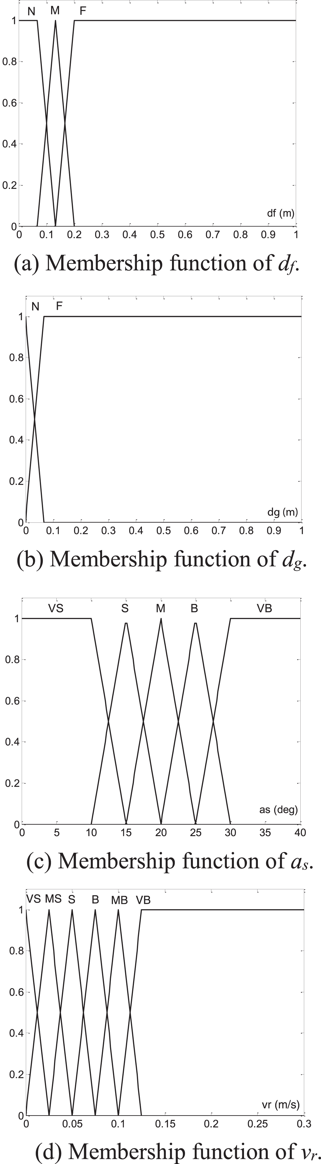
Membership functions [54].
The number of possible inputs for the variables d f , d g , and a s is 3, 2, and 5 respectively, so the number of the total fuzzy rules is 3×2×5 = 30. Based on the driving experience of drivers, when the absolute value of steering angle is big, or obstacles get close, or the target position gets close, robots should slow down to improve the safety of the system. Using the reference of the driver’s experience in dealing with these 30 situations, the fuzzy rule base of speed is concluded as shown in Table 1, and several of those rules are explained here. Rule No. 1-5: in that situation, the robot is far from both obstacles and the target position, so the robot should accelerate to improve the efficiency of completing the task. Rule No. 26–30: in that situation, the robot is close to both obstacles and the target position, so the robot should slow down to avoid collision with obstacles safely and stop at the target position smoothly. All the other rules can be explained similarly depending on the human experience [55].
Fuzzy rule base [54]
In multi-robot systems, the movement of each robot is limited by other mobile robots and complex environments, so it is difficult to establish a predetermined path for each robot when performing tasks with others. Therefore, we use a dynamic path planning method, APF, to make each robot find an collision-free path from the starting position to the target position.
With the APF, the mobile robot moves in configuration space by a field of forces, which caused by the obstacles and target positions [56]. The target exerts an attractive force to guide the robot to its destination, while the obstacle generates a repulsive force against the robot, thereby planning the direction of the robot. When the TAPF is used for mobile robot path planning, it is difficult for the robot to pass through some complex obstacles, such as U-shaped obstacles, and the task cannot be completed. Figure 2 shows the robot falls into the local minimum, where the term S is the starting position and G is the target position. To make the robot escape from the local minimum and bypass complex obstacles, the IAPF is proposed in this section.

The robot falls into the local minimum.
The attractive force (F
att
) generated by the target position in the APF defined by Kala [57] is:
Equation (1) clearly shows that the closer a robot is to the target position, the greater the attractive force will be. Therefore, when the distance between a robot and its target position is greater than the threshold d0, the attractive force is very small which makes the robot take a detour or even deviate from its target. To optimize the robot’s path, the minimum threshold value of the attractive force is set as follows:
which shows the distance between a robot and its target position is taken as d0 when d g > d0.
The repulsive force (F rep ) generated by obstacles in the APF defined by Kala [57] is:
where F rep [x, y] is the component of the repulsive force in the x-axis and y-axis directions. The term k rep is the gain factor of the repulsive force. The term k is a constant. The term θ is the moving direction of the robot. The terms d fl , d fr , d l , d r , and d f are respectively the minimum distance from the robot to the left front obstacles, to the right front obstacles, to the left obstacles, to the right obstacles, and to the front obstacles.
The function of the repulsive force is to avoid collision between robots and obstacles. The robot cannot collide with obstacles when the minimum distance between them (d min ) is greater than the threshold d 1 , so the repulsive force between them should be zero. Therefore, the function of the repulsive force is improved as:
where k fl > 1 and k fr > 1. When d min ≤d1, the term k rep works with k att to ensure that the attractive and repulsive forces are on the same order of magnitude. When d min > d 1 , the term k rep is equal to zero, so the moving direction of robots is independent of the repulsive force generated by obstacles. To get robots out of the local minimum and smooth the moving trajectory, the value of k fl should be different from that of k fr and the difference between them should be small.
The resultant force (F
res
) of the attractive and repulsive forces defined by Kala [57] is:
Figures 3 (a) and (b) show that, based on the IAPF, the robot can directly bypass the shallow U-shaped obstacle without entering the inside of it. For the deeper U-shaped obstacle, as shown in Fig. 3 (c) and (d), the robot can bypass it without falling into the local minimum.
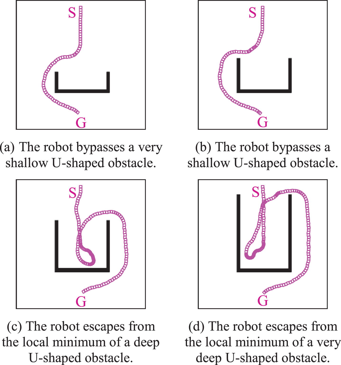
The robot bypasses the U-shaped obstacle.
In Section 2, we employ the FIS and the IAPF to avoid collision between robots and obstacles. In this section, to solve the problem of the collision between multiple mobile robots efficiently and reliably, we present a method to estimate the risk of collision between robots and a strategy to avoid the potential collision.
Collision risk assessment
To avoid collision between moving robots efficiently, we must find out the scenarios where there is risk of robots colliding with each other and estimate the risk in various scenarios.
When the robot R i is far away from R j , there is always no risk of collision between them, so the risk of collision between robots is related to the distance. To assess the collision risk, we set three distance thresholds of D1, D2, and D3, where D1 > D2 > D3, and the values of them are related to the size and speed of robots. Figure 4 shows that robots R i and R j move in the same direction while R j is in different positions. The robots in Fig. 4 (a) are at the risk of collision, but the robots shown in Fig. 4 (b) are not. Therefore, the direction and position of robots must be combined to assess the collision risk between robots.

Collision risk assessment.
The relative direction (θ
ij
) of R
j
based on the moving direction of R
i
is defined as:
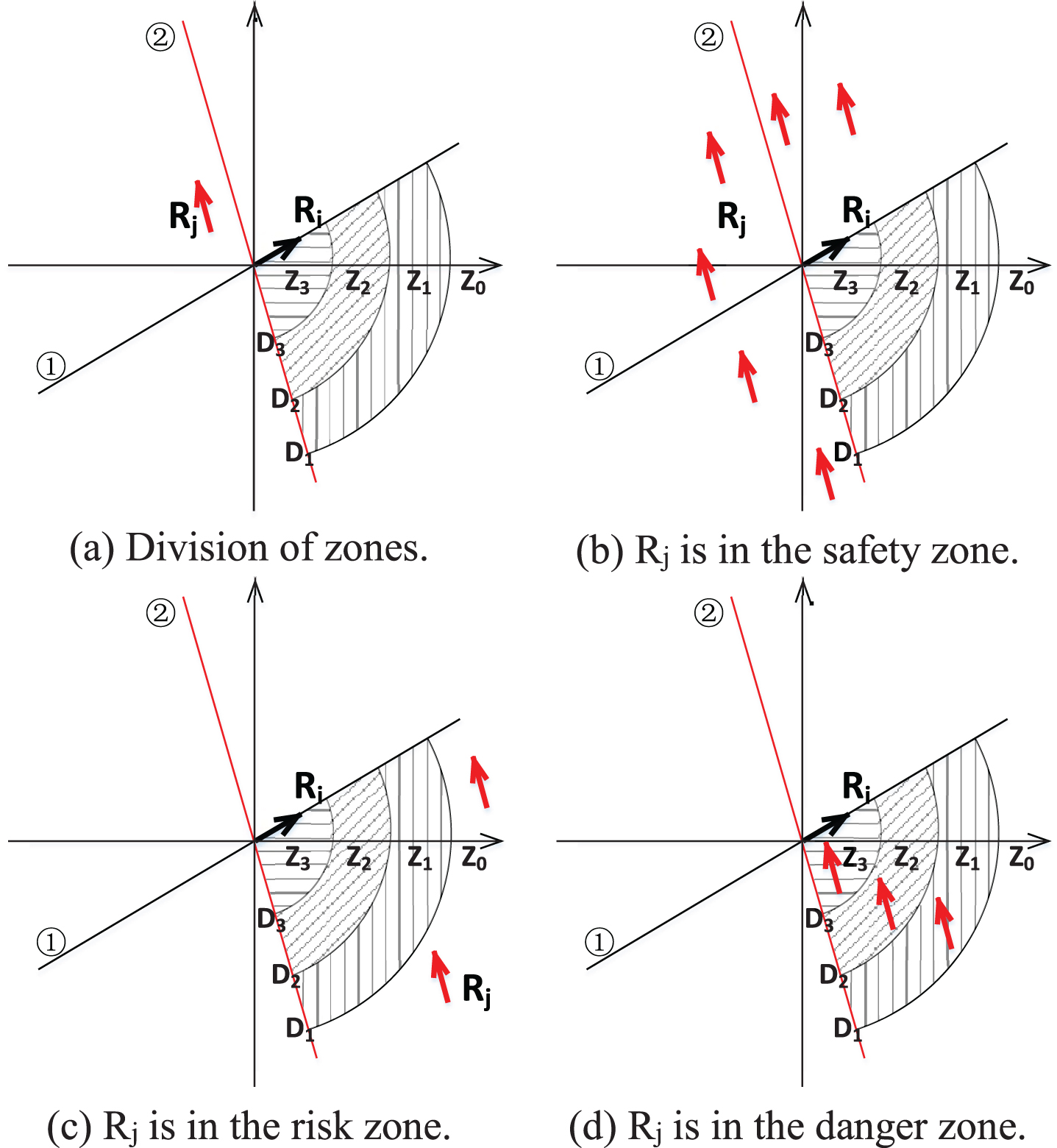
As shown in Fig. 5 (a), the black and red arrows are the moving robots R i and R j . Two straight lines are drawn through the position of R i , where the black one (line 1) is parallel to the moving direction of R i and the red one (line 2) is parallel to the moving direction of R j . The whole plane is divided into four areas by lines 1 and 2. To assess the collision risk between R i and R j , we must determine which area R j is in. Moreover, both θ i and θ ij can be divided into four numerical intervals, so there are 16 scenarios as follows.
θ i ∈[0°, 90°], θ ij ∈[0°, 90°].
Figure 5 (a) shows the scenario that θ
i
∈ [0°, 90°] and θ
ij
∈ [0°, 90°]. In the position shown in Fig. 5 (c) and (d), the robot R
j
is in the area below line 1 and to the right of line 2, and there is the risk of collision between robots. Figure 5 (b) shows that R
j
is in any position in the other three areas, and R
j
cannot collide with R
i
in this case. Therefore, it is concluded that R
j
is at the risk of colliding with R
i
only when R
j
is in the area below line 1 and to the right of line 2. For other scenarios, similar conclusions are drawn as follows. If θ
i
∈ [0°, 90°] and θ
ij
∈ [90°, 180°], as shown in Fig. 6, then R
j
is at the risk of colliding with R
i
only when R
j
is in the area below line 1 and above line 2. If θ
i
∈ [0°, 90°] and θ
ij
∈ [- 90°, 0°], as shown in Fig. 7, then Rj is at the risk of colliding with R
i
only when R
j
is in the area both above line 1 and line 2. If θ
i
∈ [0°, 90°] and θ
ij
∈ [- 180°, - 90°], as shown in Fig. 8, then R
j
is at the risk of colliding with R
i
only when R
j
is in the area above line 1 and to the right of line 2. If θ
i
∈ [90°, 180°] and θ
ij
∈ [0°, 90°], as shown in Fig. 9, then R
j
is at the risk of colliding with R
i
only when R
j
is in the area both above line 1 and line 2. If θ
i
∈ [90°, 180°] and θ
ij
∈ [90°, 180°], as shown in Fig. 10, then R
j
is at the risk of colliding with R
i
only when R
j
is in the area above line 1 and to the left of line 2. If θ
i
∈ [90°, 180°] and θ
ij
∈ [-90°, 0°], as shown in Fig. 11, then R
j
is at the risk of colliding with R
i
only when R
j
is in the area below line 1 and to the left of line 2. If θ
i
∈ [90°, 180°] and θ
ij
∈ [- 180°, - 90°], as shown in Fig. 12, then R
j
is at the risk of colliding with R
i
only when R
j
is in the area below line 1 and above line 2. If θ
i
∈ [- 90°, 0°] and θ
ij
∈ [0°, 90°], as shown in Fig. 13, then R
j
is at the risk of colliding with R
i
only when R
j
is in the area both below line 1 and line 2. If θ
i
∈ [-90°, 0°] and θ
ij
∈ [90°, 180°], as shown in Fig. 14, then Rj is at the risk of colliding with Ri only when Rj is in the area below line 1 and to the right of line 2. If θ
i
∈ [- 90°, 0°] and θ
ij
∈ [- 90°, 0°], as shown in Fig. 15, then Rj is at the risk of colliding with Ri only when Rj is in the area above line 1 and to the right of line 2. If θ
i
∈ [- 90°, 0°] and θ
ij
∈ [- 180°, -90°], as shown in Fig. 16, then Rj is at the risk of colliding with Ri only when Rj is in the area above line 1 and below line 2. If θ
i
∈ [- 180°, - 90°] and θ
ij
∈ [0°, 90°], as shown in Fig. 17, then Rj is at the risk of colliding with Ri only when Rj is in the area above line 1 and to the left of line 2. If θ
i
∈ [- 180°, - 90°] and θ
ij
∈ [90°, 180°], as shown in Fig. 18, then Rj is at the risk of colliding with Ri only when Rj is in the area above line 1 and below line 2. If θ
i
∈ [- 180°, - 90°] and θ
ij
∈ [- 90°, 0°], as shown in Fig. 19, then Rj is at the risk of colliding with Ri only when Rj is in the area both below line 1 and line 2. If θ
i
∈ [- 180°, - 90°] and θ
ij
∈ [- 180°, - 90°], as shown in Fig. 20, then Rj is at the risk of colliding with Ri only when Rj is in the area below line 1 and to the left of line 2. θ
i
∈[0°, 90°], θ
ij
∈[90°, 180°]. θ
i
∈[0°, 90°], θ
ij
∈[–90°, 0°]. θ
i
∈[0°, 90°], θ
ij
∈[–180°, –90°]. θ
i
∈[90°, 180°], θ
ij
∈[0°, 90°]. θ
i
∈[90°, 180°], θ
ij
∈[90°, 180°]. θ
i
∈[90°, 180°], θ
ij
∈[–90°, 0°]. θ
i
∈[90°, 180°], θ
ij
∈[–180°, –90°]. θ
i
∈[–90°, 0°], θ
ij
∈[0°, 90°]. θ
i
∈[–90°, 0°], θ
ij
∈[90°, 180°]. θ
i
∈[–90°, 0°], θ
ij
∈[–90°, 0°]. θ
i
∈[–90°, 0°], θ
ij
∈[–180°, –90°]. θ
i
∈[–180°, –90°], θ
ij
∈[0°, 90°]. θ
i
∈[–180°, –90°], θ
ij
∈[90°, 180°]. θ
i
∈[–180°, –90°], θ
ij
∈[–90°, 0°]. θ
i
∈[–180°, –90°], θ
ij
∈[–180°, –90°].
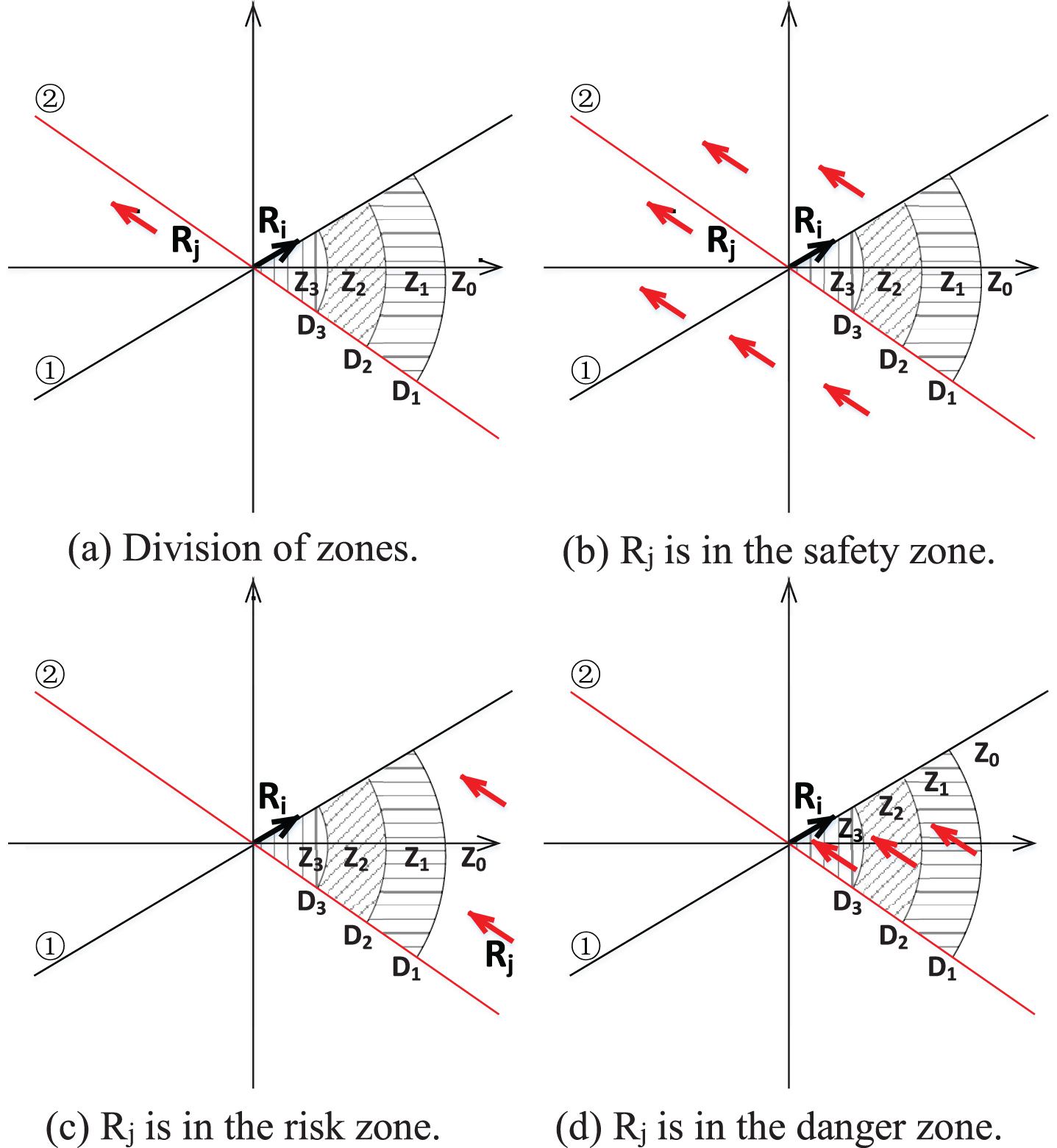
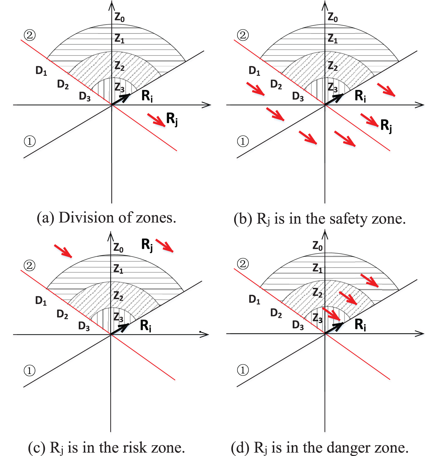
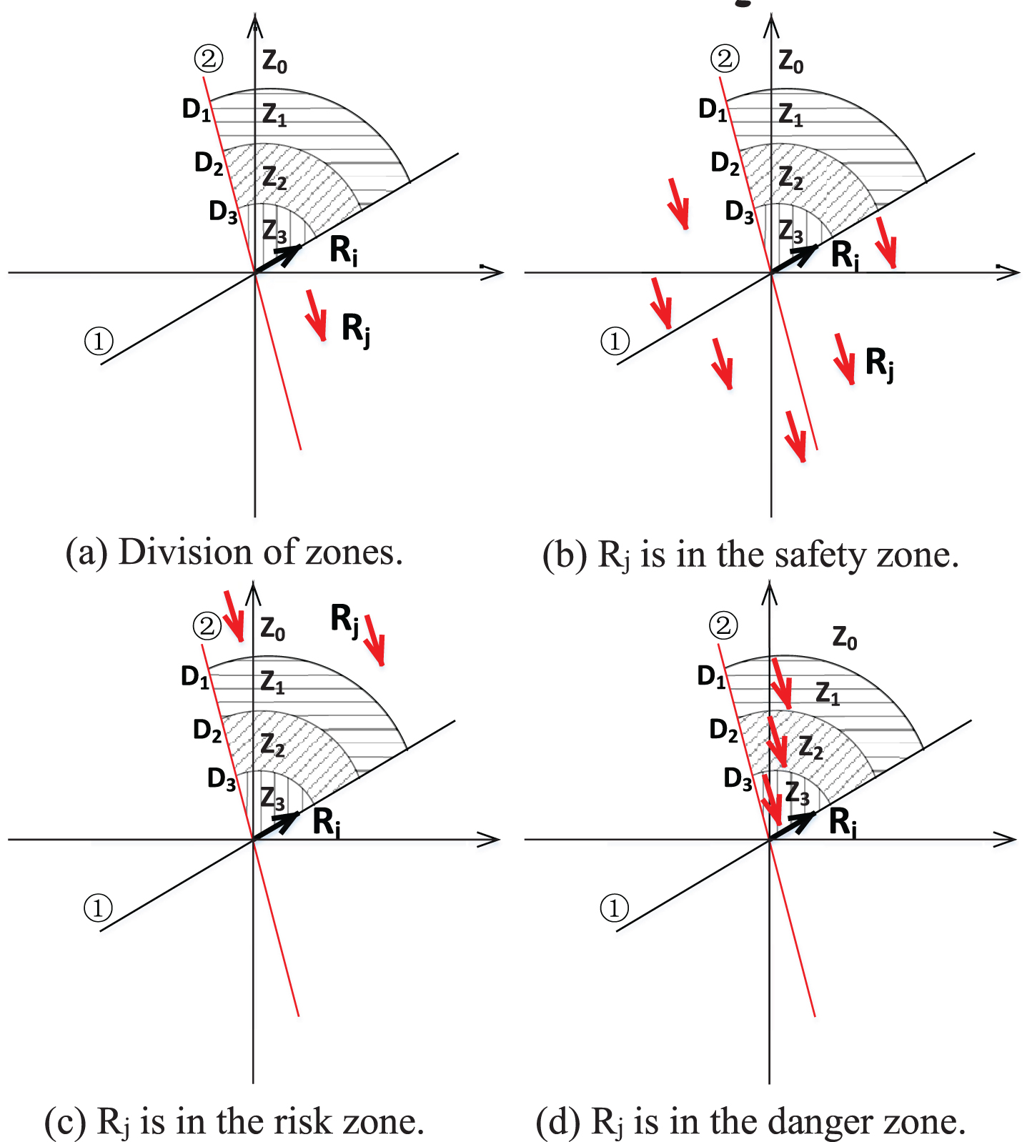
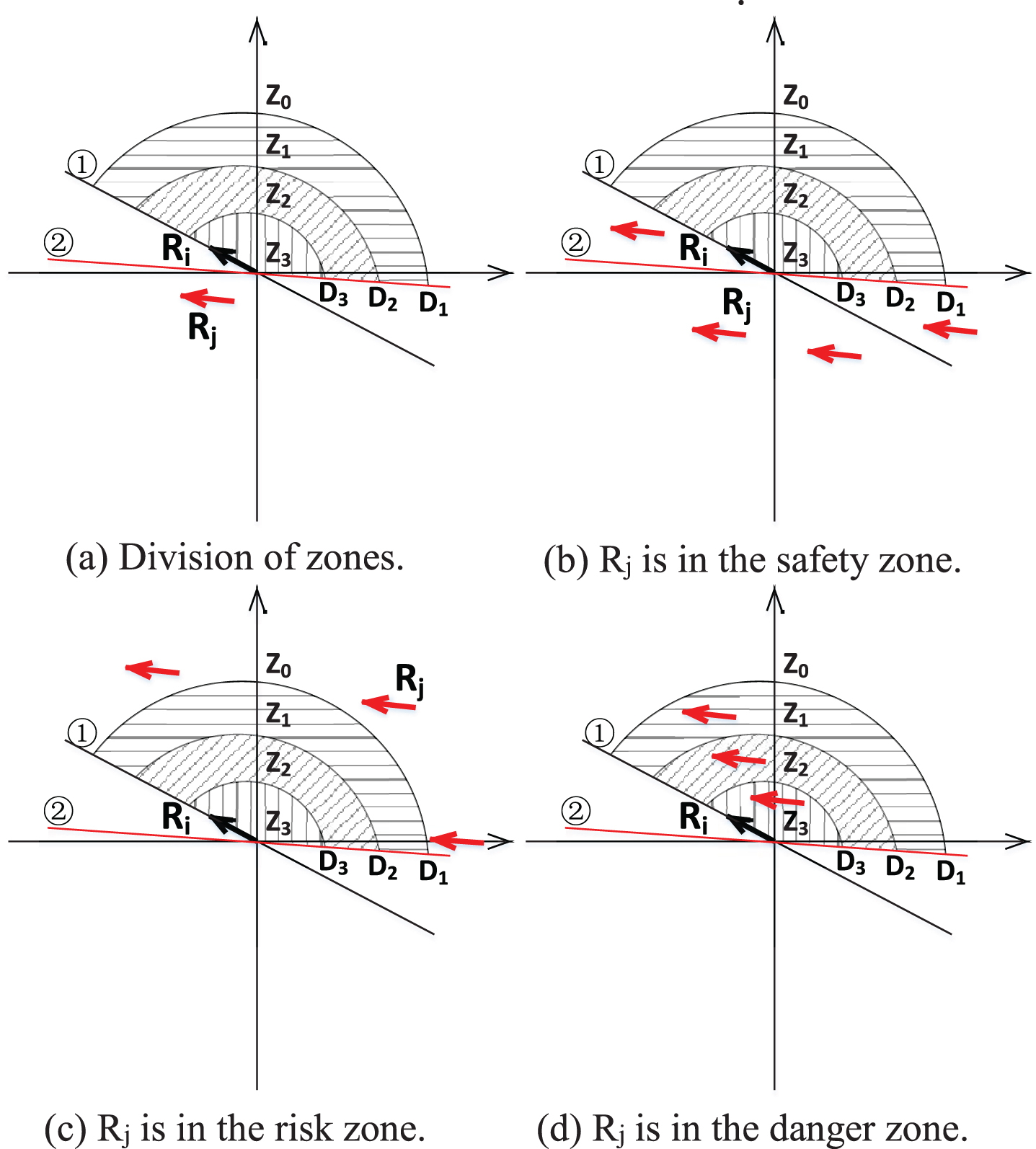
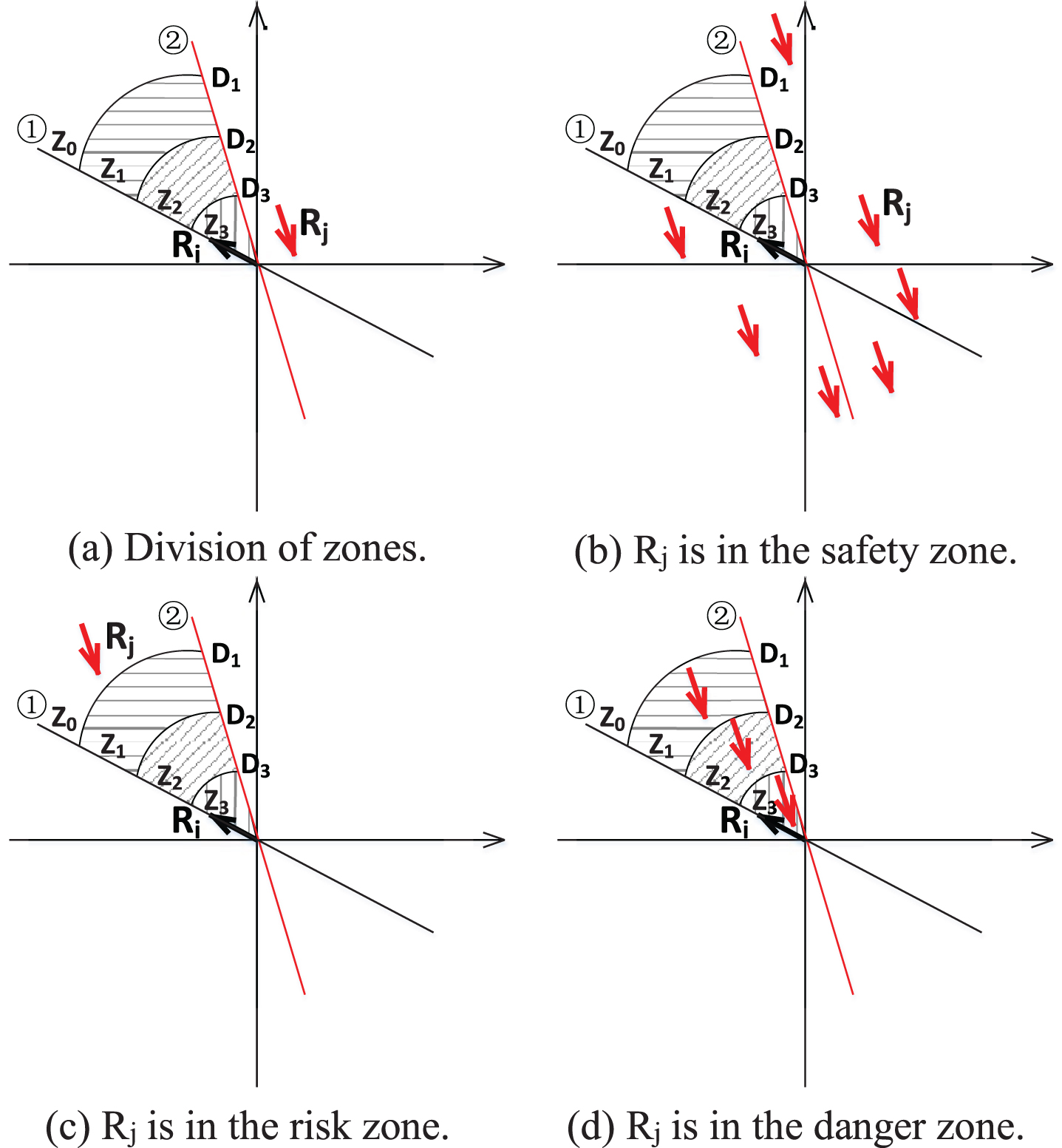
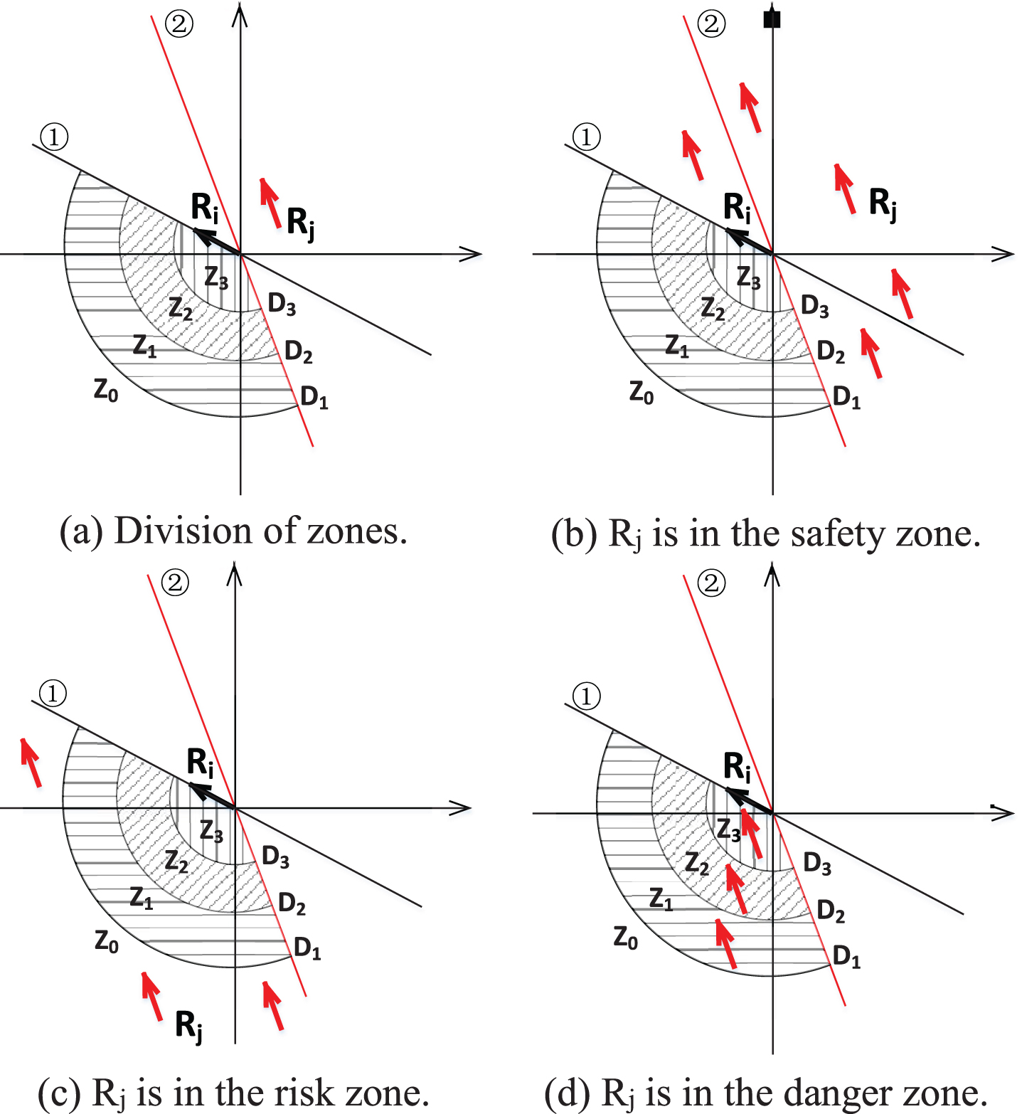
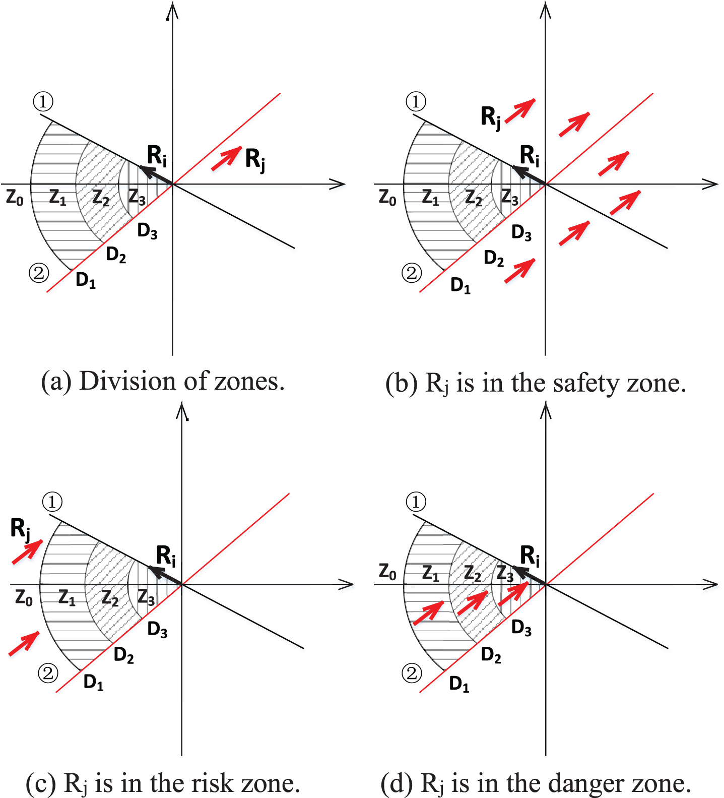
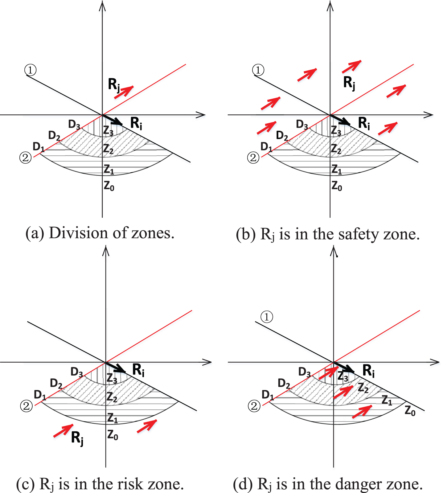
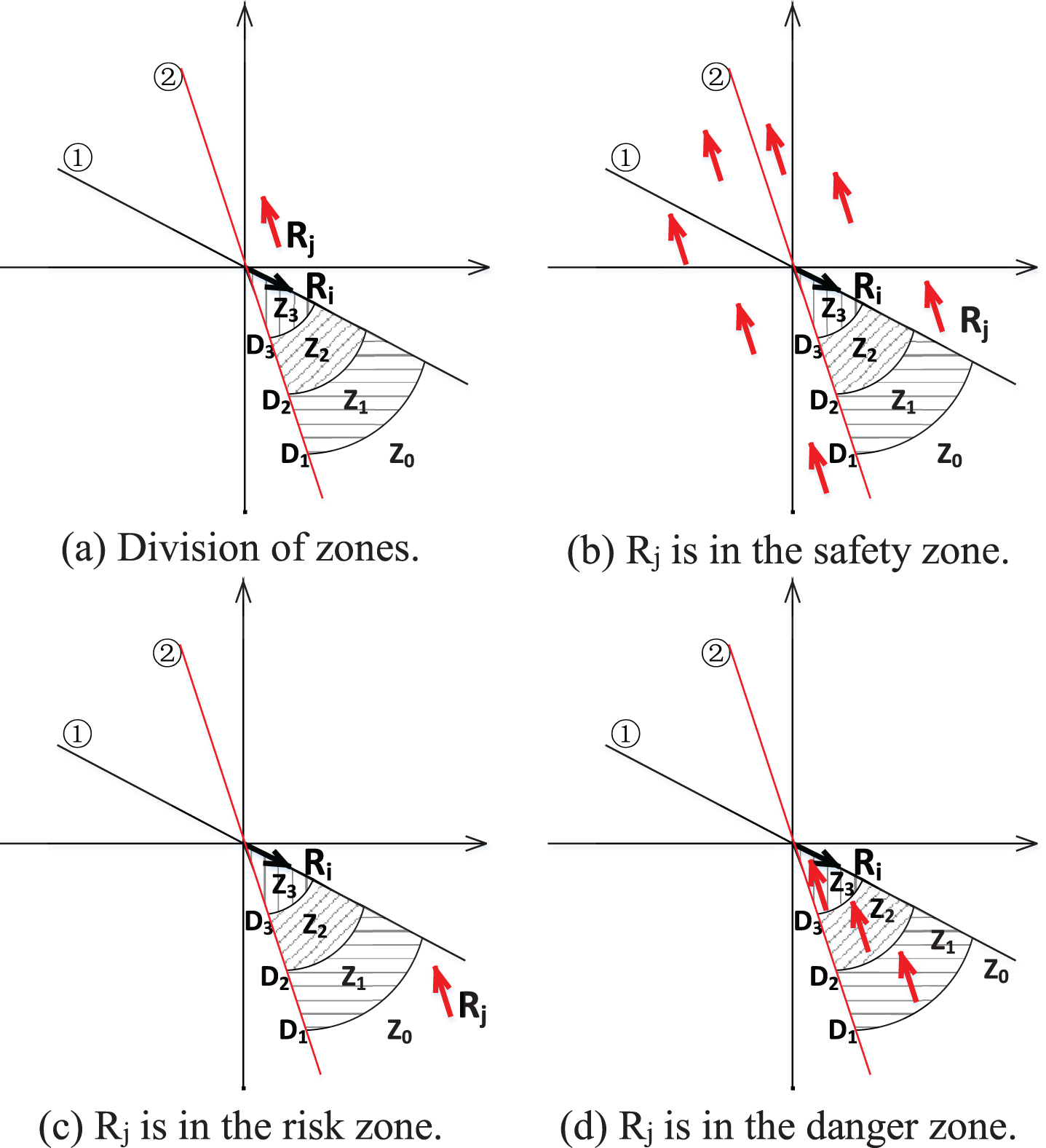
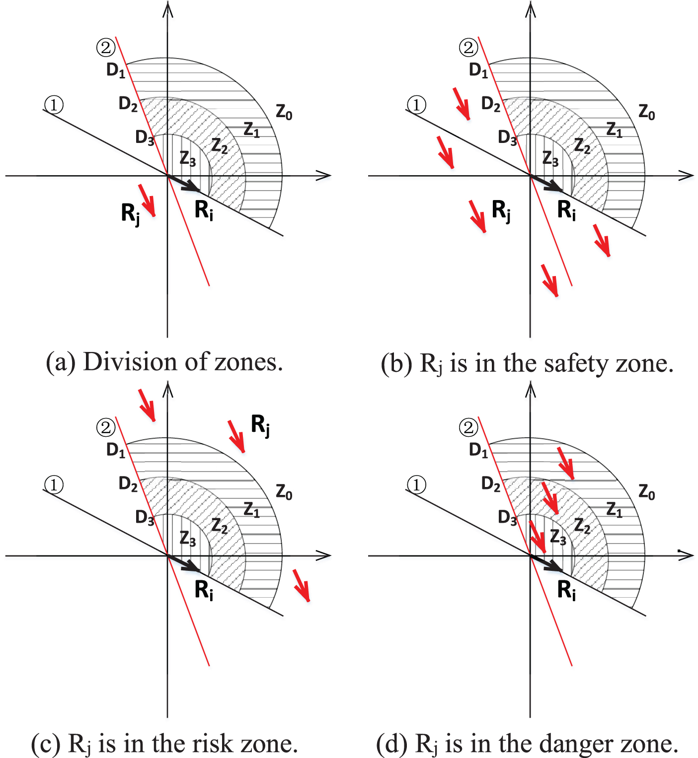
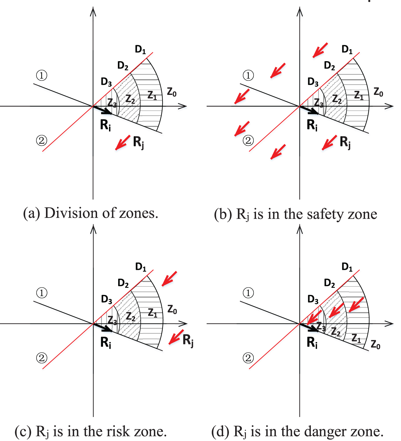
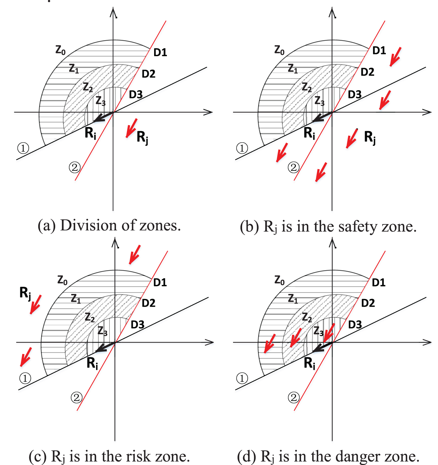
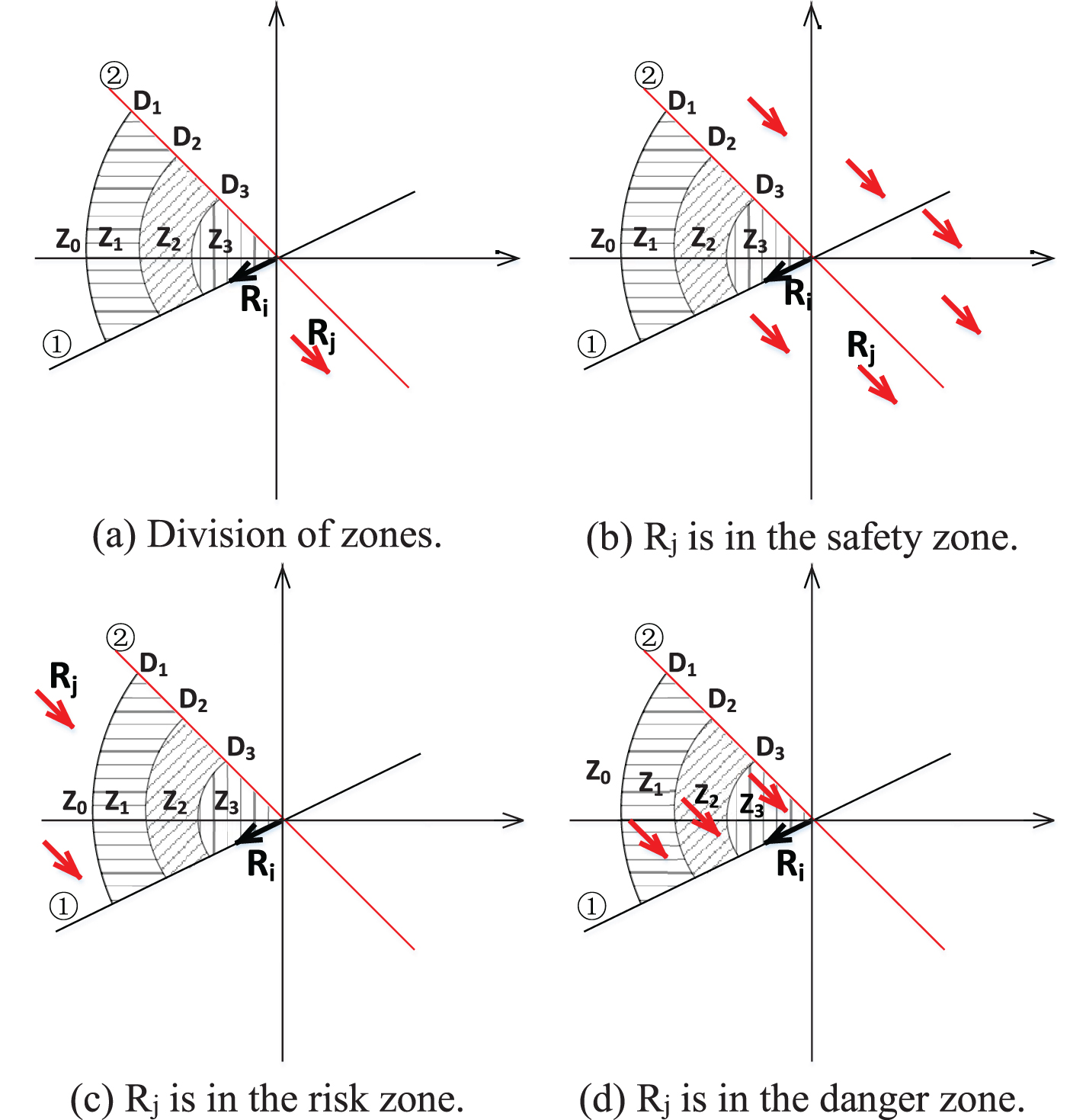
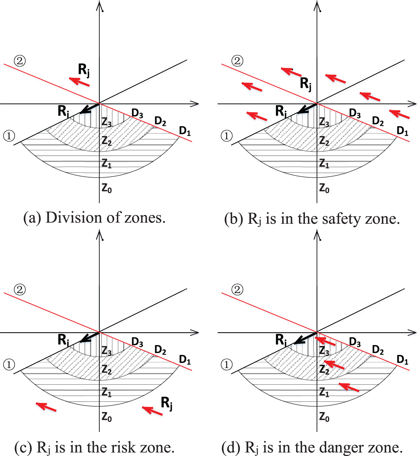
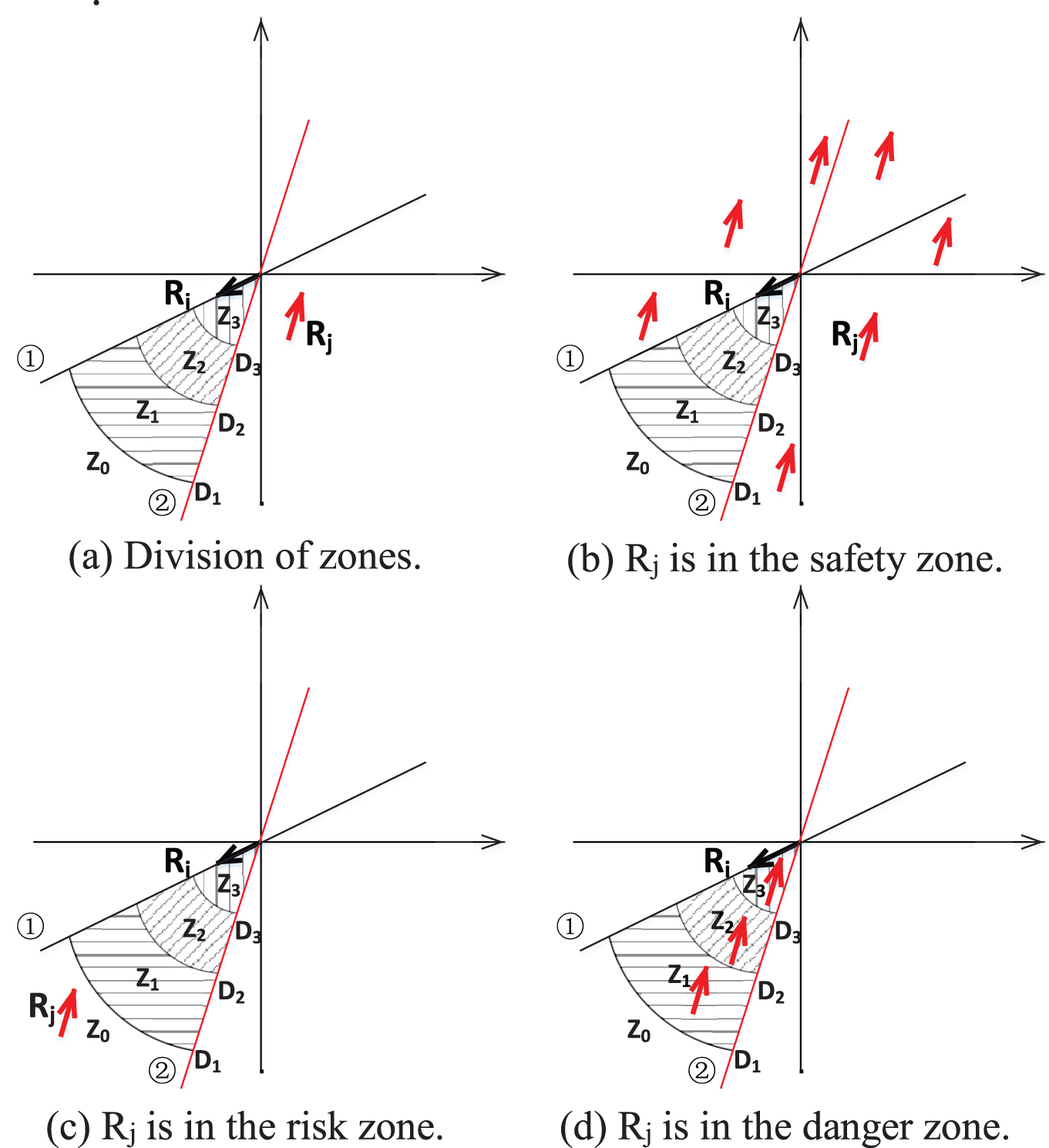
Figures 5–20 list all the scenarios based on the relative directions and positions of any two robots Ri and Rj in a multi-robot system. Figures 5–20 (b) show that Rj is in the area where Rj cannot collide with Ri. Figures 5–20 (c) and (d) show that Rj is in the area where there is the risk of collision between robots, and based on the distance between robots, the area can be further divided into Z0, Z1, Z2, and Z3. The zones Z1, Z2, and Z3 are collectively referred to as Rj’s danger zone relative to Ri, or the danger zone for short. The zone Z0 is referred to as Rj’s risk zone relative to Ri, or the risk zone for short. The zones other than Z0, Z1, Z2, and Z3 are referred to as Rj’s safety zone relative to Ri, or the safety zone for short. Due to symmetry, if Rj is in the danger zone relative to Ri, then Ri is also in the danger zone relative to Rj, and the same conclusion can be drawn for the risk zone and the safety zone. Therefore, it is concluded that Rj is at the risk of colliding with Ri only when Rj is in the danger or risk zone. When robots move from the starting position to the target position, the danger zone of any robot is refreshed in real time. If Rj is in the danger zone relative to Ri, or the distance between Ri and Rj (Dij) is less than the threshold D0 (D0 < D3), robots will implement the collision avoidance strategy to bypass each other safely.
To avoid collision between moving robots, we propose a strategy based on the IAPF. When the strategy is executed, the repulsive force will be generated between robots based on Equation (4), and robots will move in the directions that deviate from each other due to the repulsive force. To improve system security, some robots must slow down or stop to make way for other robots, so the priority of each robot is set according to the task or number. Based on the robot’s position, the strategy is divided into four stages which are both interrelated and independent of each other.
Figure 21 shows that both R2 and R3 are in Z1 of the danger zone relative to R1. Assuming that the priority of the robots is R1 > R2 > R3, then based on the stage 1, the speed of R2 and R3 are reduced to half of R1, and there is a repulsive force both between R1 and R2 and between R1 and R3. Therefore, the distance between R1 and R2 will soon be greater than D1, and R2 escapes from Z1 as shown in Fig. 21 (b). In the position shown in Fig. 21 (a), the robots R1 and R3 will move in the directions that deviate from each other due to the repulsive force based on the stage 1. The distance between R1 and R3 tends to decrease gradually when the direction is adjusted, and R3 enters Z2 of the danger zone as shown in Fig. 21 (b). To increase the adjustment time, the speed of R3 is reduced to a quarter of R1 based on the stage 2, and R3 eventually escapes from the danger zone as shown in Fig. 21 (c). When R2 and R3 escape from the danger zone and Dij≥D0, the repulsive force between robots disappears, and they continue to move toward their target position.
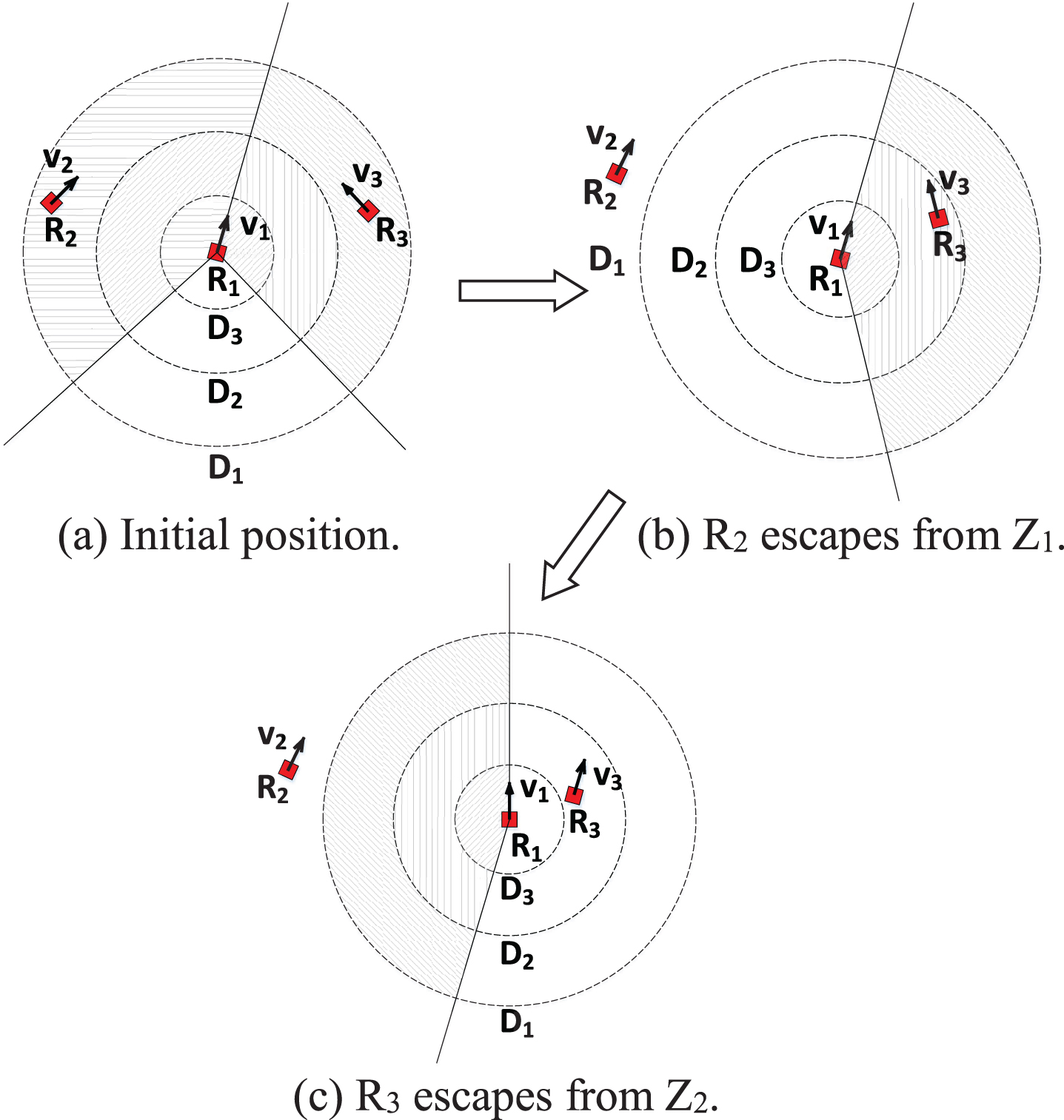
Collision avoidance between three robots.
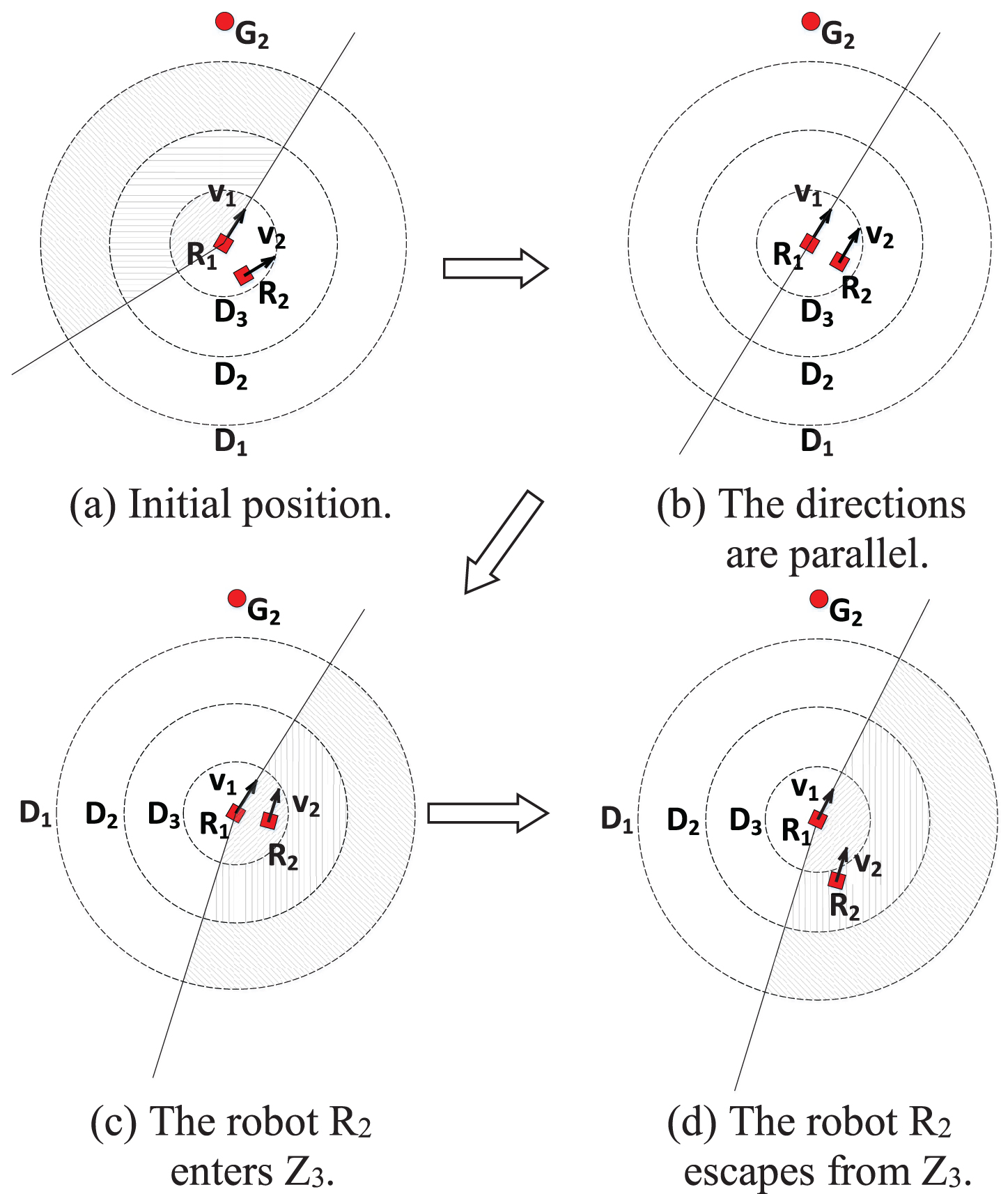
Stopping and restarting a robot requires a complicated control system and the robot is delayed in performing its tasks, so the robot will not be stopped unless in very dangerous situations as shown in the stage 3. In the position shown in Fig. 22 (a), the robots R1 and R2 are in the safety zone and D12 > D0, so the collision avoidance strategy is not implemented. However, the robot R2 will gradually shift to the left due to the attractive force from G2, and there is a risk of collision after they pass the position shown in Fig. 22 (b), where their moving directions are parallel to each other. Therefore, as shown in Fig. 22 (c), the robot R2 reaches Z3 without passing Z1 or Z2. Based on the stage 3, it stops moving and no longer starts moving again until it escapes Z3 as shown in Fig. 22 (d).
The robot R2 enters Z3 without passing Z1 or Z2.
According to the above discussion and analysis, we can see that robots can typically safely bypass each other without stopping by implementing the stages 1 and 2. However, if the collision risk is not eliminated by the two stages, or the collision risk suddenly appears when Dij<D3 as shown in Fig. 22, then the stage 3 is implemented to avoid the potential collision. Moreover, the stage 4 is used to prevent robots from getting too close to each other, improve the safety of multi-robot systems, and smooth the trajectory of each robot.
Figure 23 shows a general flowchart of a robot in a multi-robot system that will be executed in the implementation. If Ri is not in the danger zone and the distance between Ri and any other robot Rj is not less than D0, then the moving direction and speed of the robots are planned by the IAPF and the FIS. If the distance between Ri and Rj is less than D0, or Ri is in the danger zone, the collision avoidance strategy will be implemented to plan the moving direction and speed.
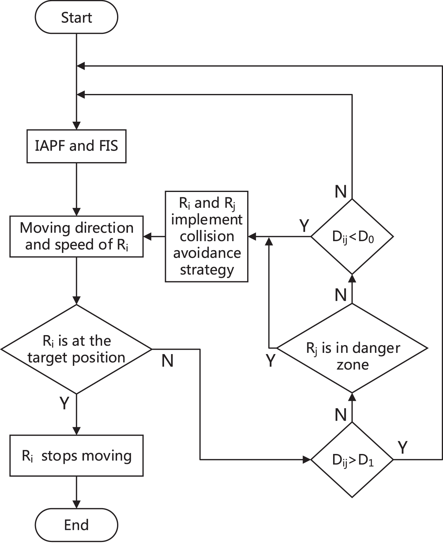
Path planning of a robot (Ri) in multi-robot systems.
To validate the effectiveness and feasibility of the collision avoidance strategy discussed in Section 3, several simulation-based experiments for collision avoidance in multi-robot systems are conducted. The simulation environment is developed using the MATLAB programming language, which is a two-dimension space of 500mm×500 mm square. Within this environment, we can set different parameters of multi-robot systems, including the number of robots, the position of obstacles, the starting position of robots, and the target position of robots. The outer contour of the robot Ri in the multi-robot system is a 10mm×10 mm square, and Si and Gi are the starting position and target position of Ri respectively. The priority of the robots in experiments is R1 > R2 > R3. The initial moving direction of each robot is toward its target position.
Collision avoidance without obstacles
Figure 24 shows the results of avoiding collision between R1 and R2 when there are no obstacles in the environment. The robot R1 starts from the top-left corner and its target position is set near the bottom-right corner. The robot R2 starts from the bottom-right corner and its target position is set near the top-left corner. In fact, the starting position of one robot is the target position of the other, so there must be a collision between them without the collision avoidance strategy. In the position shown in Fig. 24 (a), the robots R1 and R2 enter each other’s danger zone, so they will all implement the collision avoidance strategy. In the position shown in Fig. 24 (b), the robots are implementing the collision avoidance strategy. Because R1 and R2 are both on the left side of each other, they will all turn right due to the repulsive force. In the position shown in Fig. 24 (c), the robots R1 and R2 have escaped from the danger zone. However, the robot R1 is so close to R2 that D12 < D0, so based on the stage 4, the repulsive force will not disappear until Dij≥D0. Finally, the complete trajectory is shown in Fig. 24 (d).
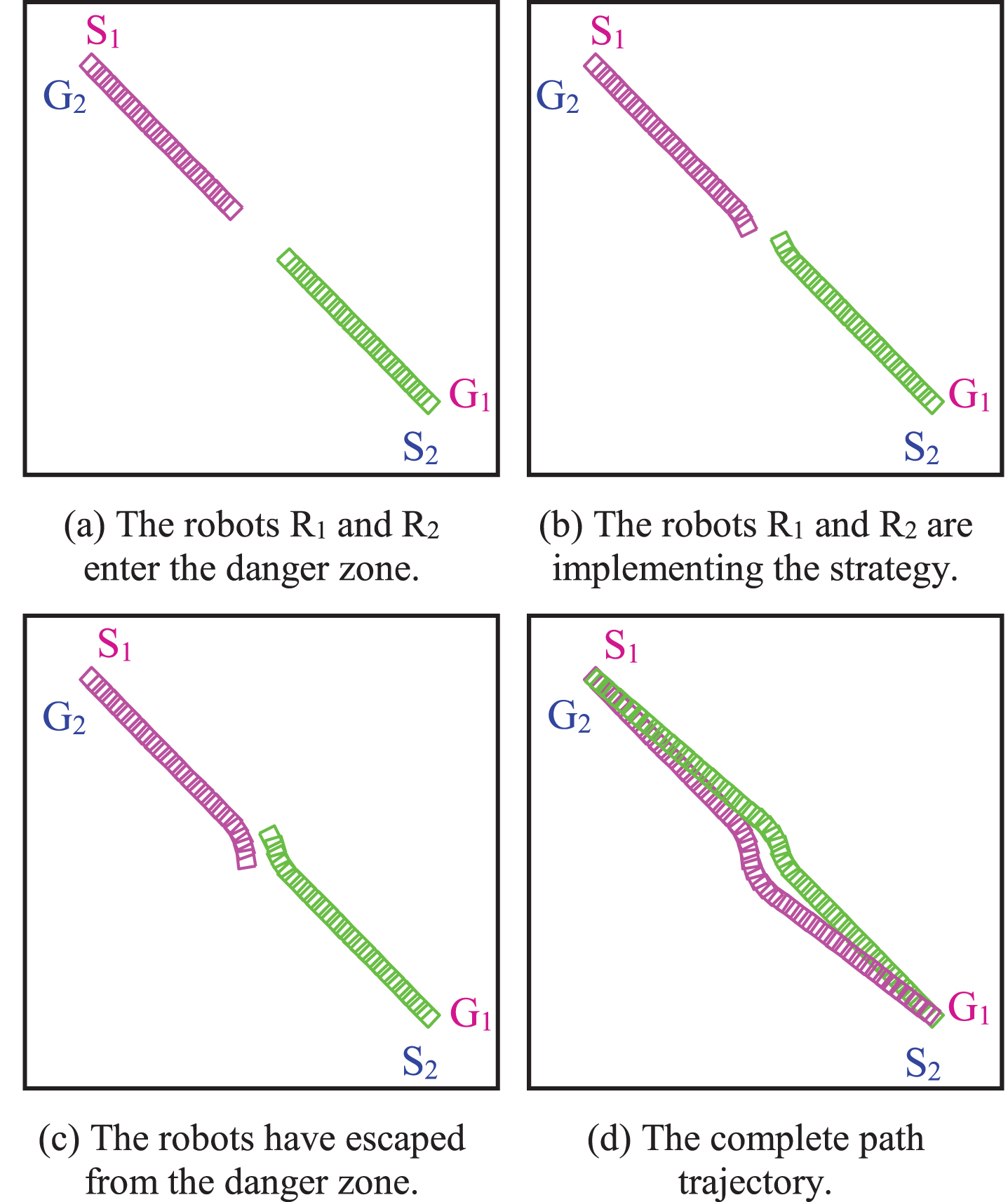
Collision avoidance between two robots.
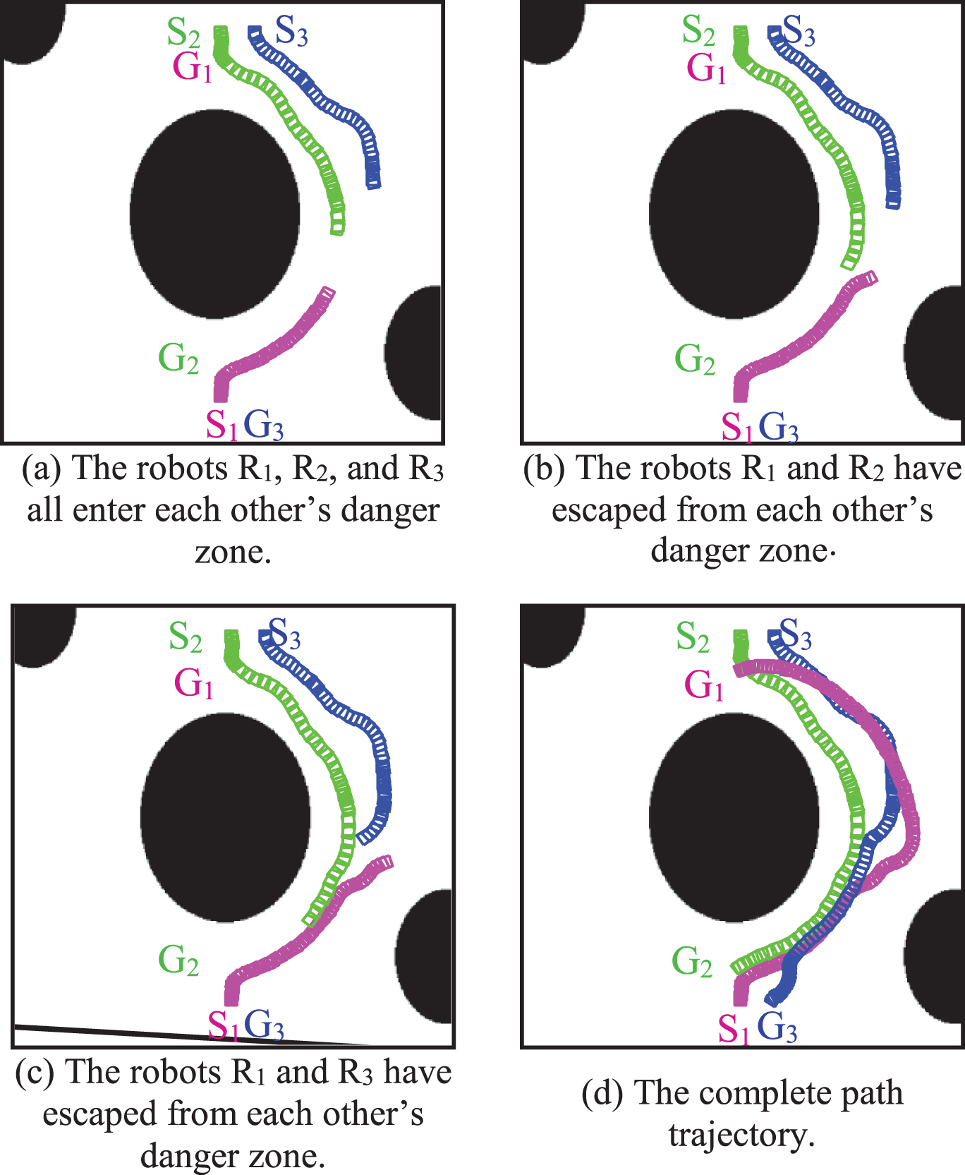
Figure 25 shows the results of collision avoidance between three robots when there are no obstacles in the environment. In the position shown in Fig. 25 (a), the robots R1, R2, and R3 all enter each other’s danger zone, so they all implement the collision avoidance strategy. Because R1 is the robot with the highest priority, the speed of R2 and R3 is reduced to lower than R1. Since R3 is closer to R1 than R2, the robot R1 will turn right due to the repulsive force from R3. In the position shown in Fig. 25 (b), the robots R1 and R3 have escaped from each other’s danger zone, but R1 and R2 are still in the danger zone of each other. In the position shown in Fig. 25 (c), the robots R1 and R2 have escaped from each other’s danger zone, while R2 and R3 are still in the danger zone of each other. Due to the repulsive force, the robot R2 will turn left and R3 will turn right as shown in Fig. 25 (d). Since the speed of R2 is higher than that of R3, the robot R2 will bypass R3 without deadlock. In the position shown in Fig. 25 (e), the robots R2 and R3 have escaped from each other’s danger zone and D23≥D0, so the repulsion between the robots disappears, and there will be no influence between the three robots until they enter the danger zone again. Figure 25 (f) shows the complete path trajectory of collision avoidance between R1, R2, and R3.
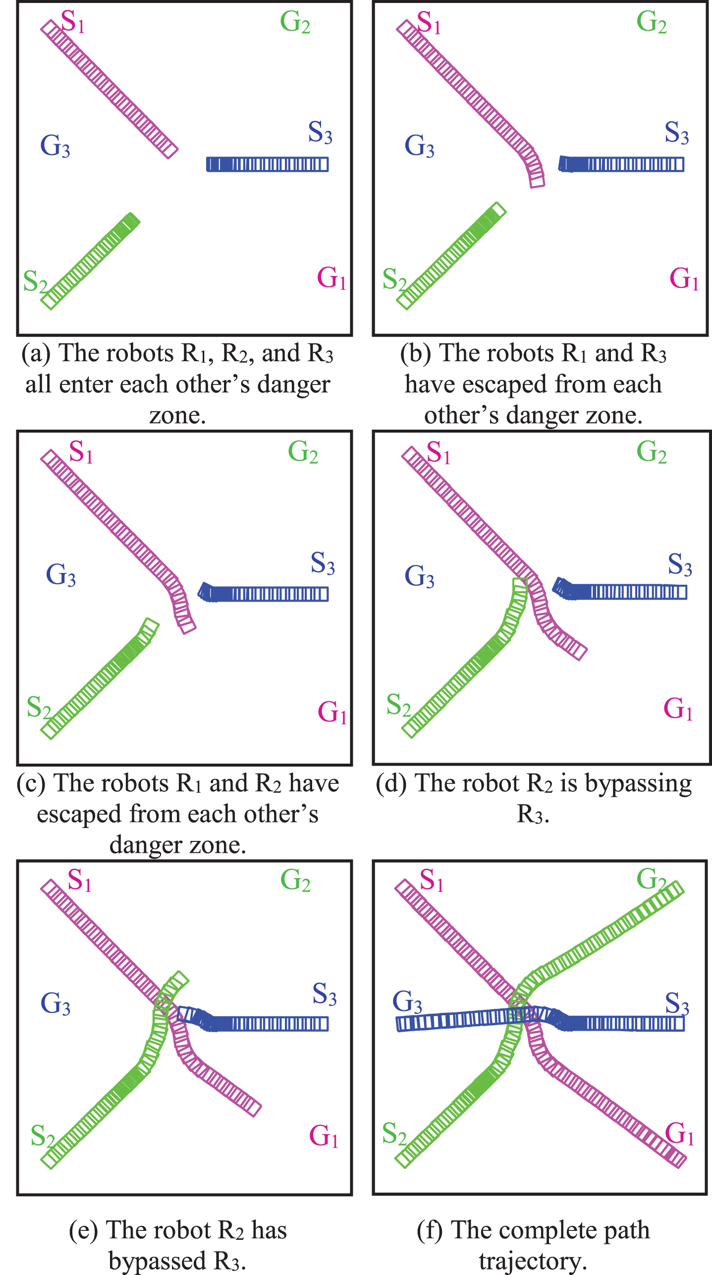
Collision avoidance between three robots.
Figure 26 is the results of collision avoidance between two robots when there are some simple obstacles in the environment. Because R1 and R2 are both close to obstacles, their speed planned by the FIS is small. The target position of each robot is in front of it, so the steering of the robots mainly depends on the repulsive force from the elliptical obstacle in front of the robots. The repulsive force on the robot is to the right due to d f l < d fr , so R1 turns to the right. Similarly, R2 will turn to the left. In the position shown in Fig. 26 (a), the robots enter each other’s danger zone, so they will all implement the collision avoidance strategy. In the position shown in Fig. 26 (b), because R1 and R2 are both on the left side of each other, they will all turn right due to the repulsive force. In the position shown in Fig. 26 (c), R1 and R2 have escaped from the danger zone of each other. Figure 26 (d) shows the complete path trajectory of R1 and R2.
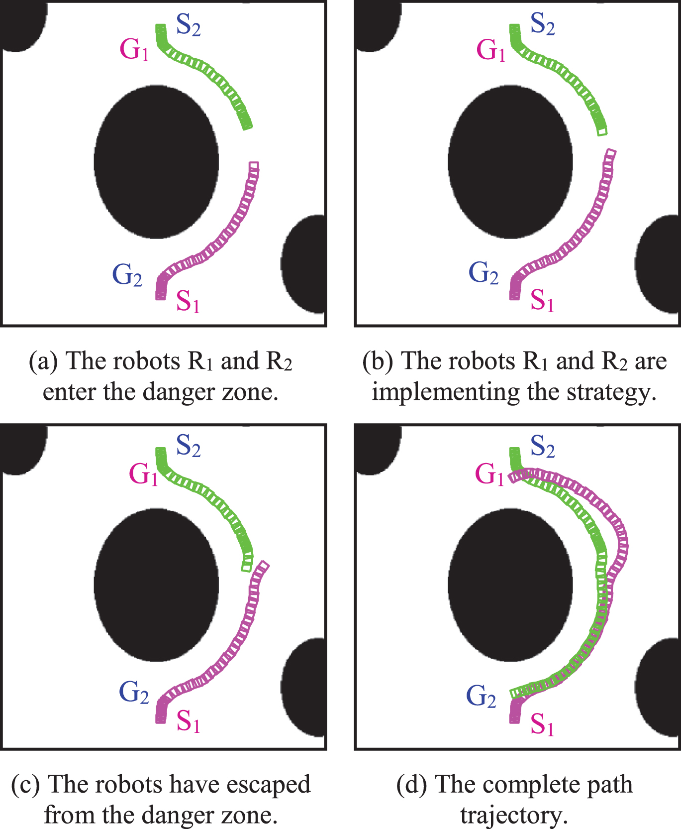
Collision avoidance between two robots.
Figure 27 shows the results for collision avoidance between three robots when there are some simple obstacles in the environment. In the position shown in Fig. 27 (a), the robots R1 and R2 enter each other’s danger zone, so they implement the collision avoidance strategy to bypass each other. In the position shown in Fig. 27 (b), the robots R1 and R2 have escaped from each other’s danger zone. In the position shown in Fig. 27 (c), the robot R1 and R3 have escaped from each other’s danger zone. Figure 27 (d) shows the complete path trajectory of collision avoidance between R1, R2, and R3.
Collision avoidance between three robots.
To validate the adaptability and flexibility of the proposed collision avoidance strategy, simulation experiments are conducted in an environment with more complex obstacles.
Figure 28 shows the results for collision avoidance between three robots when there are U-shaped obstacles and many other complex obstacles in the environment. The starting position and target position of each robot are shown in Fig. 28 (f). In the position shown in Fig. 28 (a), the robot R3 has bypassed the U-shaped obstacle. In the position shown in Fig. 28 (b), the robot R1 and R3 enter each other’s danger zone, so they will all implement the collision avoidance strategy. Because R1 is the robot with the highest priority, the speed of R3 is reduced to lower than that of R1. In the position shown in Fig. 28 (c), the robots R1 and R3 have escaped from each other’s danger zone. In the position shown in Fig. 28 (d), the robots R2 and R3 enter each other’s danger zone, and R2 will turn right and R3 will turn left due to the repulsive force from each other. Because the speed of R2 is higher than that of R3, the robot R2 will bypass R3 without deadlock as shown in Fig. 28 (e). Figure 28 (f) shows the complete path trajectory of R1, R2, and R3.
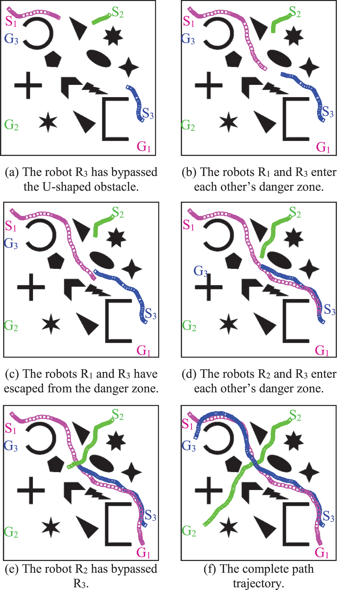
Collision avoidance between three robots.
We now compare our method, a hybridization of the IAPF and the FIS, against the other two algorithms: FIS and APF. Table 2 represents the starting position and target position of each robot. Figure 29 shows the simulation results of five robots at the same starting position and target position under the three methods.
The initial position and target position of each robot
The initial position and target position of each robot
The performance of the simulation results is first analyzed in the terms of whether the robot can reach the target position, which is the foundation for the robot to complete a given task. As shown in R1 in Fig. 29, the robot using our proposed method passes the U-shaped obstacle safely, while the robot using the FIS collides with the obstacle, and the robot using the APF falls into the local minimum. As shown in R2 in Fig. 29, for complex obstacles, the robot using our method successfully bypasses it, while the robot using the FIS or the APF collides with the obstacle. As shown in R5 in Fig. 29, whose starting position is very close to the obstacle, the robot using our method passes the obstacle without collision, while the robot using the FIS or the APF cannot bypass the obstacle safely. Therefore, the hybridization of the IAPF and the FIS improves the robot’s ability to cope with complex obstacles and enhances the security performance of the system.
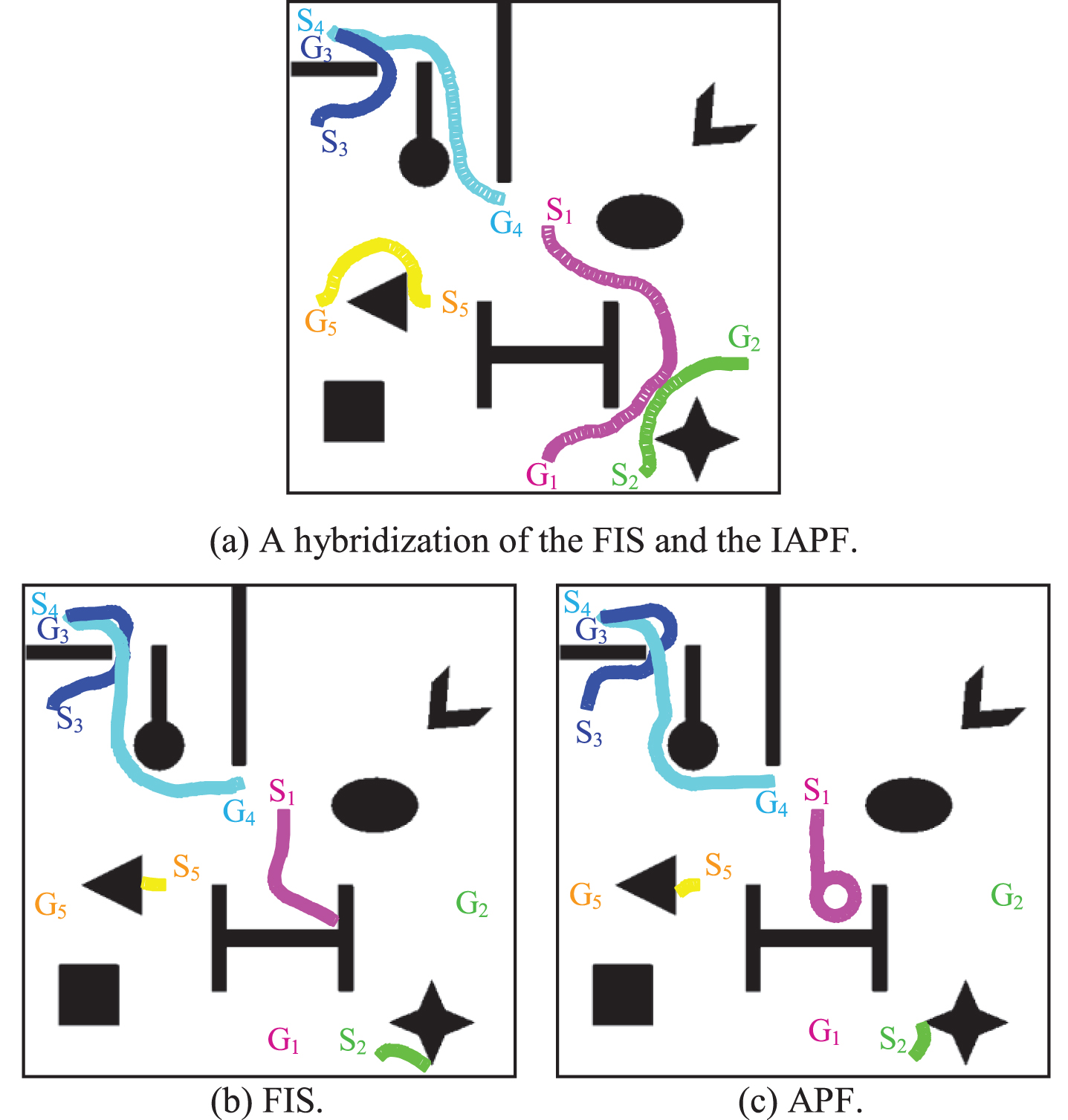
The trajectory of five robots under different algorithms.
Then the performance of the simulation results is analyzed in the terms of trajectory distance, by which we can able to minimize the energy consumption. The trajectory distance traveled under different algorithms is shown in Table 3, where the term “×” represents that the robot cannot reach its target position without collision. Taking R1 and R2 as an example, the trajectory distance of the robot using our proposed method is shorter than that using the FIS or the APF. Therefore, compared the other two algorithms, the path length of robot using our proposed algorithm is shorter.
The trajectory distance traveled under different algorithms
A hybridization of the IAPF and the FIS was proposed to plan a collision-free smoothness optimal or suboptimal path from the given starting position to goal position for each robot in the multi-robot system. The results obtained from the experimental work are in good agreement with the proposed algorithm. The performance between different algorithms has been compared. It is concluded that our proposed algorithm outperforms over other algorithms used for multi-robot path planning. However, in this paper, both the environment and obstacles are static relative to the robot, whereas other robots are dynamic for original robots. In the future, work will be carried out using dynamic obstacles other than robots such as running vehicles, animals and onboard camera during multi-robot path planning. Moreover, we will attend to improving our method for a more complex environment. Finally, because the control method, mechanics of robot motion, and environmental detection precision is different in realistic multi-robot systems, it is challenging to implement the strategy in a real system. Therefore, in the future, further efforts are needed to validate the proposed strategy in a physical multi-robot system.