Technical and economic optimization of natural gas transmission network operation to balance node delivery flow rate and operation cost

Abstract

Natural gas transmission network is the major facility connecting the upstream gas sources and downstream consumers. In this paper, a multi-objective optimization model is built to find the optimum operation scheme of the natural gas transmission network. This model aims to balance two conflicting optimization objective named maximum a specified node delivery flow rate and minimum compressor station power consumption cost. The decision variables involve continuous and discrete variables, including node delivery flow rate, number of running compressors and their rotational speed. Besides, a series of equality and inequality constraints for nodes, pipelines and compressor stations are introduced to control the optimization results. Then, the developed optimization model is applied to a practical large tree-topology gas transmission network, which is 2,229 km in length with 7 compressor stations, 2 gas injection nodes and 20 gas delivery nodes. The ɛ-constraint method and GAMS/DICOPT solver are adopted to solve the bi-objective optimization model. The optimization result obtained is a set of Pareto optimal solutions. To verify the validity of the proposed method, the optimization results are compared with the actual operation scheme. Through the comparison of different Pareto optimal solutions, the variation law of objective functions and decision variables between different optimal solutions are clarified. Finally, sensitivity analyses are also performed to determine the influence of operating parameter changes on the optimization results.

Keywords

Natural gas transmission network operation optimization compressor station multi-objective optimization

Nomenclature

Parameters

A₁-A₁₁

BWRS equation coefficients

A_h, B_h, C_h, D_h

Head characteristic equation coefficients

A_e, B_e, C_e, D_e

Efficiency characteristic equation coefficients

A_su, B_su, C_su, D_su

Surge limit characteristic equation coefficients

A_st, B_st, C_st, D_st

Stonewall limit characteristic equation coefficients

Constant, 0.0384 (m²· s $\cdot \sqrt{K} / kg$ )

Diameter (m)

Compressor Power price (¥/(kW·h))

Compressor head (kJ/kg)

\bar{k}

Adiabatic index of natural gas

Pipeline length (m)

Natural gas mass flow rate (kg/s)

Pressure (MPa)

Natural gas volume flow rate (m³/s)

Natural gas constant, 8.314 (J/(mol·K))

Reynolds number

Natural gas flow temperature (K)

Compressor running time (h)

Compressor power (kW)

Compressibility factor

Greek symbols

Flow direction relationship parameter

Relative density of natural gas

number of running compressors

Pipeline absolute roughness (m)

Efficiency (%)

Friction coefficient

Dynamic viscosity of natural gas (Pa·s)

Density (kmol/m³)

Compressor rotational speed (r/min)

Subscripts

Efficiency

Head

Node

Gas injection node

Gas delivery node

Gas transshipment node

Compressor station arc

Pipeline arc

Stonewall

Surge

Superscript

Pipeline inlet

avg

Average

Pipeline outlet

Compressor station

Discharge side of compressor

Injection

Isentropic

mech

Mechanical

out

Delivery

Pipeline

Suction side of compressor

1 Introduction

Natural gas is a clean and efficient low-carbon energy source, and it plays an increasingly significant role in global energy consumption. A large amount of natural gas is widely transported and distributed via pipeline networks because of their convenience, economy and reliability [1]. Natural gas pipeline networks are usually classified into gathering, transmission and distribution networks. Transmission networks are the main ways of connecting the upstream gas field and downstream users, which have the characteristics of long distance, large transmission amount and high operating pressure.

A gas transmission network is mainly made up of gas sources, pipelines, compressor stations (CSs), valves, distribution centers, etc. The schematic of a representative gas transmission network is shown in Fig. 1. In the network, pipelines are mainly responsible for the transmission of natural gas form gas sources to distributing centers. Then, distribution centers supply gas to Consumers, Which usually including residential, industrial and electric generation consumers. By means of a valve, gas operators can restrict or direct the gas flow from one pipeline to another. In addition, gas pressure continuously decreases because of the friction with the pipeline wall when it flows along the pipeline. Therefore, there are compressor stations along the network to pressurize natural gas to ensure the safe transmission.

Fig. 1

Schematic of a representative gas transmission network.

Generally, gas transmission network optimization is mainly divided into design optimization and operation optimization. The former one refers to the proper selection of layout, materials and dimensions of the network, as well as the location and scale of each station [2, 3]. While the latter one means optimizing the operating parameters of the system with known conditions of the network structure and layout to obtain the optimal operating plan, and thus meeting economic or technical goals [4]. Obviously, during the planning and construction phase of the gas transmission network, operators will pay more attention to the design optimization of gas network. However, after the gas transmission network is completed and put into operation, it will operate for several decades. During this period, operators will develop feasible network operation plans based on user consumption needs and network transmission capacity. Different operation schemes will lead to different economic benefits and operating conditions. In a large and complex gas pipeline network, even a small percentage improvement in operating conditions will bring huge economic value. Therefore, in the operation life cycle of gas transmission network, operators are most concerned about the optimization of network operation. The research on this problem has important technical and economic value, which is also the motivation of this article.

Nowadays, with the sustained growth of the global consumption of natural gas, its position in the world’s energy structure continues to rise. According to the World Energy Outlook 2018 [5], the annual global natural gas production is expected to exceed 4×10¹²m³ in 2022. It is also expected that by the end of 2023, the average annual growth rate for the entire forecast period is expected to reach 1.6%. By 2040, natural gas will overtake coal to become the world’s second largest energy source, with an increase of nearly 50% [6]. In this context, gas transmission networks, as the most important and economical means of transportation, should increase the gas transmission capacity of the pipeline as much as possible to meet the growing demand of consumers. However, with the increase of pipeline gas transmission capacity, compressor stations need to provide higher gas delivering pressure, resulting in greater energy consumption and operation cost. Previous studies have shown that the operating costs of CSs make up for 25–50% of the total system operating costs [7]. Moreover, higher operating pressure will place higher requirements on the performance of equipment. Hence, how to balance the relationship between the consumer gas delivery volume and operating costs is a major challenge for pipeline operators.

In order to find an optimal network operation condition between the consumer gas transmission volume and operating cost, this paper built a multi-objective optimization model considering maximum delivery flow rate of a specified gas delivery node and minimum compressor station power consumption cost. Then, the ɛ-constraint method is used to convert this bi-objective optimization model into a series of single-objective optimization models, and the optimization models is solved on the GAMS (General Algebraic Modeling System) optimization platform. Since the established optimization model belongs to the MINLP problem, the platform chooses the DICOPT solver suitable for this type of problem to solve it. After nearly 30 years of development, GAMS has been successfully applied to mathematical optimization problems in various fields, and it has powerful advantages in the extensiveness, stability and convenience of optimization solutions.

1.1 Literature review

Many researches have been conducted in optimization of gas transmission network operation. Some published review literatures describe developments in this area. Rios-Mercado and Borraz-Sanchez [1] provides a review on the most relevant research works conducted to solve natural gas transportation problems via pipeline systems. Wu et al. [8] provides a review on the progress related to the steady-state operation optimization models of natural gas pipelines as well as corresponding solution methods based on stochastic optimization algorithms. Next, this article will introduce the related research progress of gas transmission network operation optimization from the aspects of mathematical model types, solving methods and objective functions.

Long before, researchers have recognized operation optimization models of gas transmission network as a nonlinear programing (NLP) model because of the nonlinear pipeline and compressor constraints [9]. Besides, if consider the RCs number in each station, the model then turns into a mixed-integer NLP (MINLP) model. Hence, the models can be classified into NLP and MINLP model depending on the decision variable. NLP models assume that the RCs number in the network is known in advance. Besides, discrete variables that represent the number of compressors to be turned on are introduced into MINLP models.

The solving method of gas transmission network operation optimization have been studied by many researchers. However, there is still existing a tremendous potential. This is because different methods have different advantages, disadvantages, and range of applications [10]. Dynamic programming (DP) is the first method applied to the operating optimization of gas network. In 1968, Wong and Larson [11] firstly applied DP to the minimum fuel cost problem. However, as the dimension of the model increases, the computation quantity of the DP algorithm increases exponentially. So, it is difficult to solve the problem of large pipeline optimization. Percell and Ryan [12] studied the generalized reduced gradient (GRG) for non-cyclic structures. The GRG method conquered the dimension problem of DP algorithm and is suitable for complex structural networks. Futhermore, the linear programming (LP) was applied to deal with this problem [13], by transforming the non-linear model into a linear model. The advantage of LP is that the calculation speed is usually faster. However, if the initial value is not chosen properly, the solution of the algorithm is easy to fall into a inferior local optimal solution.

Different from above traditional deterministic methods, some emergent metaheuristic optimization algorithms have shown many advantages in terms of dealing with the large-scale pipeline and MINLP problem [8]. In recent years, some studies applied metaheuristic algorithms in this area effectively, for instance, ant colony optimization [14], Genetic Algorithm [15, 16], Simulated Annealing [17], Particle Swarm Optimization [18], and their extensions.

Gas transmission networks are usually characterized as a complex and huge system. We are supposed to fully consider the economic, safety and social benefits of the plan in the process of developing the network operation plan. Therefore, operation optimization of the gas transmission network is essentially a multi-objective optimization problem. However, because of the difficulty and computational complexity of multi-objective optimization techniques, most previous scholars only conducted single-objective optimization studies. The main objective functions are: delivery flow rate maximization [16], line pack maximization [19, 20], power consumption minimization [21, 22], profits maximization [23], etc. Some common optimization objectives in natural gas network operation optimization are summarized in Fig. 2.

Fig. 2

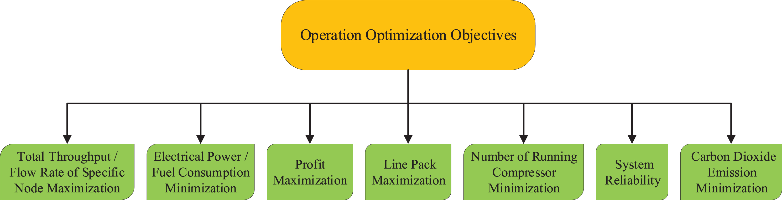
Common objectives of gas transmission network operation optimization.

With the development of multi-objective optimization algorithms in recent years, some researchers have begun to apply multi-objective optimization techniques to gas transmission network operation optimization problems. Wu et al. [24] utilized weighted sum method and inertia-adaptive PSO algorithm to solve the bi-objective model considered maximum operation benefit and maximum flow rate. Alinia Kashani and Molaei [25] built a MINLP model to minimizing operating cost, maximizing throughput and maximizing line pack. The developed model was solved by NSGA-II. Demissie et al. [26] presented a multi-objective model for different pipeline configurations of linear, tree and looped topologies. They took energy consumption minimization and transport flow rate maximization as objective functions. Su et al. [27] developed a multi-objective optimization method to trade-off reliability and power demand of natural gas pipeline network. Nevertheless, there is still a big gap in the study of multi-objective optimization compared with single objective optimization.

1.2 Contributions

The main contributions of this paper are summarized below. Firstly, previous studies generally applied a large number of assumptions and simplified pipeline and compressor station models, leading to the reduction of accuracy and practicability of the model. For instance, Wu et al. [24] simplified the compressor model without considering the working rule and working interval of compressors. Demissie et al. [26] supposed that the gas Compressibility factor is an average constant and did not consider its variety in different pipelines. In this paper, a relatively precise and realistic optimization model of compressor stations and pipelines is established. This model considers the working rule and working feasible area of the compressor. The gas density, friction factor and compressibility factor are accurately calculated, thus replacing the method of picking empirical constants directly. Besides, the previous optimization of natural gas network operations mostly belonged to single-objective optimization problems. Even for multi-objective optimization problems, most of them focused on maximizing the total pipeline output [24 –26]. Unfortunately, few researches have considered maximizing the delivery flow rate for a specific consumer. Hence, this paper focuses on the delivery flow rate at a specific gas delivery node GDN. And an optimization model considering maximum delivery flow rate of specified GDN and minimum CS power consumption cost is built. Finally, given that previous research usually selected small pipeline examples with simple structure and few users [25, 26], few studies were conducted on real-world large pipelines, and failed to effectively combine multi-objective optimization with engineering practice. In view of this, this study selected a practical large-scale gas transmission network as the optimization object. This pipeline is 2,229 km in length, and contains 7 CSs, 2 GINs and 20 GDNs.

Consequently, the main purpose of this paper is to establish a multi-objective operation optimization model for large gas transmission network with considering two conflict objectives of minimum CS energy consumption cost and maximum delivery flow rate of a specific GDN. Then ɛ-constraint method and GAMS/DICOPT solver were adopted to solve the multi-objective optimization problem.

The rest of the article is structured as follows: Section 2 defines the system assumptions, bi-objective functions, constraints, and decision variables. Section 3 studies optimization method and solver. Section 4 discusses bi-objective optimization results and sensitivity analyses. Finally, Section 5 summarizes the full text.

2 Mathematical model

In order to facilitate mathematical modeling and solution, the natural gas transmission network is simplified into a system consisting of nodes and arcs in this paper. Let G = (N, M) be a directed graph representing a natural gas transmission network, where N is the set of nodes representing interconnection points, and V is the set of arcs representing either pipelines or compressor stations. The nodes set N = N_ii ∪ N_id ∪ N_it consists of gas injection nodes (GIN) subset N_ii with elements ii representing gas sources, gas delivery nodes (GDN) subset N_id with elements id representing distributing centers, gas transshipment nodes (GTN) subset N_it with elements it representing valves or arcs connection points. Let M = M_j ∪ M_k be partitioned into a set of compressor station arcs M_j with elements j and a set of pipeline arcs M_k with elements k. Based on these definitions, this section illustrates the System assumptions, objective functions and constraints of the operation optimization model in details.

2.1 System assumptions

(1) Steady state flow

When natural gas flow in pipelines, it generally in an unstable state, in which the hydraulic and thermal parameters of gas vary over time. However, when it comes to the annual or monthly operational planning of the gas transmission network system, due to the long time, the system instability has little impact on the research results and can be ignored. Therefore, the optimization problem of long-term natural gas network operation is usually simplified to a steady state.

(2) Isothermal flow

Generally, natural gas flow temperature changes along pipelines, and finally approximate the environment temperature where the pipeline is constructed. However, practical applications show that the gas temperature changing value is much smaller than the Kelvin temperature reference value (273.15 K), and the variability within a certain range has little impact on the fluid pressure and flow rate. Hence, this paper adopted the assumption of gas flow in pipelines isothermally, and the temperature is 293.15 K.

2.2 Multi-objective functions

(1) Maximize delivery flow rate of a specified GDN

Various gas supply ways may exist for a certain gas user. With the continuous increase of natural gas consumption in the future, gas transmission network, as the most important and economical means of transportation, should increase its gas transmission capacity as much as possible to meet natural gas demand of users. Hence, the delivery flow rate at the specified GDN maximization might be considered as an objective function, which can be modeled as Equation (1). $max f_{1} = Q_{id}^{out} id \in N_{id}$ (1)

Where $Q_{id}^{out}$ is the delivery flow rate at a specified GDN, m³/s.

(2) Minimize CS power consumption cost

Minimum operating cost is a major interests of the network company. Gas transmission network operating cost mainly includes CS power consumption cost, CS equipment maintenance and repair costs, pipeline’s maintenance cost, and so on. This paper mainly studies the variable operation cost of network without considering the maintenance and repair cost of equipment. The variable operation cost is mainly made up of the CS power consumption cost. Therefore, this paper chooses to minimize the CS power consumption cost as another optimization goal. The objective function is represented as Equation (2). $min f_{2} = \sum_{j = 1}^{M_{j}} E_{j} δ_{j} W_{j} t_{j} j \in M_{j}$ (2) Where E_j is the power price of the jth CS, ¥/(kW·h); δ _j is the RCs number of the jth CS; W_j is the single compressor power of the jth CS, kW; t_j is the compressor running time of the jth CS, h.

2.3 Equality constraints

(1) Node flow balance equation

The node flow balance equation is derived from the law of mass conservation. At any node, that is for all GINs, GDNs and GTNs, the inlet flow and outlet flow should be equal. This constraint can be expressed as Equation (3). $Q_{i}^{in} - Q_{i}^{out} + \sum β_{ij} Q_{j}^{CS} + \sum β_{ik} Q_{k}^{p} = 0 i \in N$ (3)

Where $Q_{i}^{in}$ is the injection flow rate of the ith node, m³/s; $Q_{i}^{out}$ is the injection flow rate of the ith node, m³/s; $Q_{j}^{CS}$ is the flow rate of the jth CS connected to the ith node, m³/s; β_ij is the fluid direction coefficient, if the gas flows into ith node, β_ik = 1, otherwise, β_ik = - 1; $Q_{k}^{p}$ denotes the flow passes through the kth pipeline connected to the ith node, m³/s; and β_ik has the same meaning as β_ij.

(2) Gas flow equation

When natural gas flows in the pipeline, part of the energy will be lost due to the roughness of the inner wall of the pipe, causing the pressure gradual loss along the pipeline. The general flow equation describes the relationship between the gas flow rate $Q_{k}^{p}$ and inlet pressure $P_{k}^{a}$ , outlet pressure $P_{k}^{b}$ of the pipe, which is derived from one-dimensional momentum conservation equation [28]. The general flow equation is expressed as Equation (4). $Q_{k}^{p} = C \sqrt{\frac{[(P_{k}^{a})^{2} - (P_{k}^{b})^{2}] D_{k}^{5}}{λ_{k} Z_{k}^{avg} Δ {TL}_{k}}} k \in M_{k}$ (4)

Where $Q_{k}^{p}$ is the flow rate of the kth pipeline, m³/s; $P_{k}^{a}$ is the inlet pressure of the kth pipeline, Pa; $P_{k}^{b}$ is the outlet pressure of the kth pipeline, Pa; C is the constant, 0.0384 (m²·s $\cdot \sqrt{K}$ /kg); D_k is the diameter of the kth pipeline, m; λ_k is the friction coefficient of the kth pipeline; $Z_{k}^{avg}$ is the average compressibility factor of the kth pipeline; Δ is the relative density of gas; T is gas flow temperature, K; L_k is the length of the kth pipeline, m.

Based on the inlet pressure $P_{k}^{a}$ and outlet pressure $P_{k}^{b}$ of pipeline, the average pressure $P_{k}^{avg}$ can be calculated by Equation (5). $P_{k}^{avg} = \frac{2}{3} (P_{k}^{a} + \frac{(P_{k}^{b})^{2}}{P_{k}^{a} + P_{k}^{b}})$ (5)

(3) Friction factor equation

The friction factor λ is a significant gas flow parameter, which is correlated with the gas flow state and pipeline’s roughness. According to the Reynolds number and relative roughness of pipe, the gas flow state is divided into laminar flow and turbulent flow. While the turbulent flow is divided into three areas: hydraulic smooth zone, mixed friction zone and resistance square zone. Different equations have different scope of application. These equations mainly include Weymouth, Pan(A), Pan(B), AGA, Colebrook, etc. Colebrook equation (Equation (6)) is commonly used because of the wide range of application and high accuracy, which is derived from the Prandtl hydraulic smooth tube equation and the Nikolas complete rough tube equation [29]. $\frac{1}{\sqrt{λ_{k}}} = - 2 lg (\frac{ɛ_{k}}{3.7 D_{k}} + \frac{2.51}{{Re}_{k} \sqrt{λ_{k}}}) k \in M_{k}$ (6) Where ɛ_k is the inner wall equivalent roughness of the kth pipeline, m; Re_k is the reynolds number of the kth pipeline, which can be calculated by Equation (7). ${Re}_{k} = 1.536 \frac{Q_{k}^{p} Δ}{D_{k} μ}$ (7)

Where Δ is the relative density of gas; μ is the dynamic viscosity of natural gas, Pa·s.

(4) Compressibility factor equation

Compressibility factor Z indicates the volume deviation of the actual gas from the ideal gas after compression by the same pressure, which is a correction factor that must be considered when gas flows in a pipe. BWRS equation is widely adopted to the calculation of compressibility factor due to the character of high computational accuracy and wide applicability. BWRS equation is obtained by modifying the BWR equation. This equation has 11 light hydrocarbon component coefficients, each of which can be obtained by the relevant calculation formula and calculation rules. Since pipelines at different locations have different operating pressure, especially for huge gas pipeline systems, there is a large gap between the starting and ending pressure. Therefore, this model will calculate the average compression factor $Z_{k}^{avg}$ of each pipeline separately, which can be calculated by Equation (8). $\begin{matrix} Z_{k}^{avg} = 1 + (A_{1} + \frac{A_{2}}{RT} + \frac{A_{3}}{{RT}^{3}} + \frac{A_{4}}{{RT}^{4}} + \frac{A_{5}}{{RT}^{5}}) \\ \times ρ_{k}^{avg} + (A_{6} - \frac{A_{7}}{RT} + \frac{A_{8}}{{RT}^{3}}) \times (ρ_{k}^{avg})^{2} \\ + \frac{A_{9}}{RT} (A_{7} + \frac{A_{8}}{T}) \times (ρ_{k}^{avg})^{5} + \frac{A_{10} (ρ_{k}^{avg})^{2}}{{RT}^{3}} \\ (1 + A_{11} (ρ_{k}^{avg})^{2}) exp (- A_{11} (ρ_{k}^{avg})^{2}) k \in M_{k} \end{matrix}$ (8)

Where $Z_{k}^{avg}$ is the average compressibility factor of the kth pipeline; A₁-A₁₁ is the BWRS equation coefficients; R is the constants related to the state of natural gas, 8.314 J/(mol·K); T is natural gas flow temperature, K; $ρ_{k}^{avg}$ is the gas average density of the kth pipeline, kmol/m³, which can be calculated by Equation (9). $ρ_{k}^{avg} = \frac{P_{k}^{avg}}{Z_{k}^{avg} RT}$ (9)

It’s worth noting that the calculation equations for the friction factor and the compressibility factor are implicit equations, which cannot be directly solved. Hence, Newton–Raphson method is applied in the modeling process.

(5) Compressor performance equation

The compressor is one of the most complex equipment in a natural gas network. The compressor characteristic curve refers to the relationship between head H_j, isentropic compression efficiency $η_{j}^{is}$ , suction flow rate $Q_{j}^{s}$ and rotational speed ω_j. The maps describe the operating performance of the compressor and estimate its operating parameters. The relationship between pressure head H_j, suction flow rate $Q_{j}^{s}$ and speed ω_j is shown in Fig. 3(a). In addition, the relationship between the isentropic compression efficiency $η_{j}^{is}$ and the suction flow rate $Q_{j}^{s}$ and rotational speed ω_j is also represented in Fig. 3(b). The characteristic curves denote the operating performance of the compressor and estimate its operating parameters.

Fig. 3

Compressor characteristic curves: (a) H_j, $Q_{j}^{s}$ , ω_j; (b) $η_{j}^{is}$ , $Q_{j}^{s}$ , ω_j.

In the process of modeling, a mathematical language is needed to describe the compressor maps. Hence, the characteristic curves are often fitted to a polynomial equation called compressor characteristic equation. In these equations, $H_{j} / ω_{j}^{2}$ , $Q_{j}^{s} / ω_{j}$ , $η_{j}^{is}$ are selected as equation variables, and coefficients A_h, B_h, C_h, D_h, A_e, B_e, C_e, D_e are determined by nonlinear least square method. The head characteristic equation and the efficiency characteristic equation are expressed by Equations (10) and (11) separately [30]. $\frac{H_{j}}{ω_{j}^{2}} = A_{h} + B_{h} (\frac{Q_{j}^{s}}{ω_{j}}) + C_{h} (\frac{Q_{j}^{s}}{ω_{j}})^{2} + D_{h} (\frac{Q_{j}^{s}}{ω_{j}})^{3} j \in M_{j}$ (10) $η_{j}^{is} = A_{e} + B_{e} (\frac{Q_{j}^{s}}{ω_{j}}) + C_{e} (\frac{Q_{j}^{s}}{ω_{j}})^{2} + D_{e} (\frac{Q_{j}^{s}}{ω_{j}})^{3}$ (11)

Where H_j is the compressor pressure head of the jth CS, kJ/kg; ω_j is the compressor rotational speed of the jth CS, r/min; $Q_{j}^{s}$ is compressor actual suction flow rate of the jth CS, m³/s; $η_{j}^{is}$ is isentropic compression efficiency of the jth CS, %; A_h, B_h, C_h, D_h is head characteristic equation coefficients; A_e, B_e, C_e, D_e is efficiency characteristic equation coefficients.

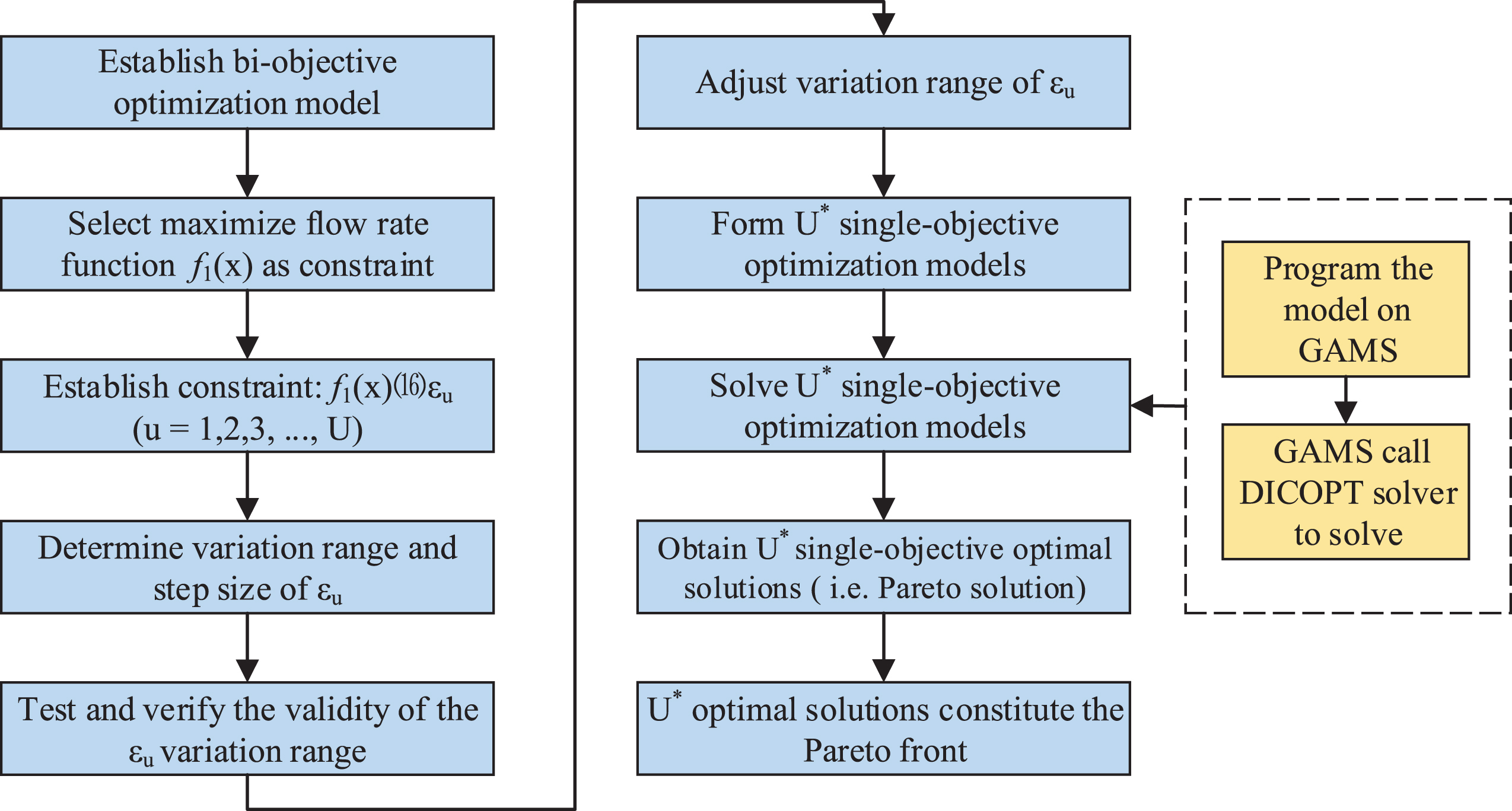
When a compressor is working, if the suction flow rate $Q_{j}^{s}$ is too low, surge might occur; and if the flow rate is too high, stonewall might occur. Both phenomena can affect the performance of the compressor. Therefore, it is necessary to restrict the flow rate and control the compressor within a certain working range. The surge and stonewall limit curve are on the left and right sides of Fig. 4(a) respectively. The limitation of the suction gas flow $Q_{j}^{s}$ (Equation (14)) can be obtained by fitting the surge limit curve and stonewall limit curve to the polynomial equations Equations (12) and (13). $Q_{j, su}^{s} = A_{su} + B_{su} ω_{j} + C_{su} ω_{j}^{2} + D_{su} ω_{j}^{3}$ (12) $Q_{j, st}^{s} = A_{st} + B_{st} ω_{j} + C_{st} ω_{j}^{2} + D_{st} ω_{j}^{3}$ (13) $Q_{j, su}^{s} ⩽ Q_{j}^{s} ⩽ Q_{j, st}^{s}$ (14)

Fig. 4

Procedures of solving the model with the ɛ-constraint method.

Where $Q_{j, su}^{s}$ is the compressor surge limit flow rate of the jth CS, m/s; $Q_{j, st}^{s}$ is the compressor stonewall limit flow rate of the jth CS, m/s; A_su, B_su, C_su, D_su is the surge limit characteristic equation coefficients. A_st, C_st, D_st is the stonewall limit characteristic equation coefficients.

The discharge pressure $P_{j}^{d}$ of the compressor thus can be calculated after calculating the compressor head, which is defined as Equation (15). $H_{j} = Z_{j}^{s} RT \frac{\bar{k}}{\bar{k} - 1} [(\frac{P_{j}^{d}}{P_{j}^{s}})^{\frac{\bar{k} - 1}{\bar{k}}} - 1]$ (15)

Where $Z_{j}^{s}$ is the gas compressibility factor at compressor inlet side of the jth CS; $\bar{k}$ is gas adiabatic index; $P_{j}^{s}$ is the compressor suction pressure of the jth CS, MPa; $P_{j}^{d}$ is the compressor discharge pressure of the jth CS, MPa.

Finally, the compressor power W_j can be calculated by the mass flow M_j and head H_j. The compressor power calculation formula is as Equation (16). $W_{j} = \frac{M_{j} H_{j}}{η_{j}^{is} η_{j}^{mech}}$ (16) Where W_j is the compressor power of the jth CS, kW; M_j is the compressor mass flow rate of the jth CS, kg/s; $η_{j}^{is}$ is the isentropic compression efficiency of the jth CS, %; $η_{j}^{mech}$ is the compressor mechanical efficiency of the jth CS, %.

2.4 Inequality constraints

(1) Node flow rate constraint

As a resource, the flow of natural gas into the pipeline over a period of time $Q_{ii}^{in}$ is constrained by the maximum production or processing capacity of the producing area. In addition, for different regions and different types of natural gas users, there are different consumption demands. Therefore, at each GDN, the gas distribution volume $Q_{id}^{out}$ should be greater than the minimum volume. The related constraints can be described as Equations (17) and (18). $Q_{ii, min}^{in} ⩽ Q_{ii}^{in} ⩽ Q_{ii, max}^{in} ii \in N_{ii}$ (17) $Q_{id, min}^{out} ⩽ Q_{id}^{out} ⩽ Q_{id, max}^{out} id \in N_{id}$ (18)

Where $Q_{ii}^{in}$ is the injection flow rate of the mth GIN, m³/s; $Q_{ii, min}^{in}$ and $Q_{ii, max}^{in}$ are the minimum and maximum allowable injection flow rate of the mth GIN, m³/s; $Q_{id}^{out}$ is the delivery flow rate of the ith GDN, m³/s; $Q_{id, min}^{in}$ and $Q_{id, max}^{in}$ are the minimum and maximum allowable delivery flow rate of the mth GDN, m³/s.

(2) Node pressure constraint

Similarly, gas sources or users have certain requirements on the pressure P_i. The pressure at each node of the pipeline can be expressed as Equation (19). $P_{i, min} ⩽ P_{i} ⩽ P_{i, max} i \in N$ (19)

Where P_i is the pressure of the ith node, MPa; P_i,min is the minimum allowable pressure of the ith node, MPa; P_i,max is the maximum allowable pressure of the ith node, MPa.

(3) Pipeline pressure constraint

Natural gas flows in the pipe under pressure, and the inner pressure causes stress to the pipe wall. If the stress reaches the yield strength of the pipe, it would cause permanent deformation of the pipe and eventually cause damage to the pipe. Therefore, to ensure the safe transportation of natural gas, maximum allowable operational pressure (MAOP) parameter needs to be introduced to ensure the safe transportation of natural gas. The pipeline pressure constraint is expressed as Equation (20). $P_{k} ⩽ MAOP k \in M_{k}$ (20)

Where P_k is the pressure of the kth pipeline, MPa; MAOP is the pipeline maximum allowable operational pressure.

(4) Compressor rotational speed constraint

Compressor rotational speed is related to equipment performance and is within a certain limitation. Maximum and minimum rotational speed of compressors is expressed as Equation (21). $ω_{j, min} ⩽ ω_{j} ⩽ ω_{j, max} j \in M_{j}$ (21)

Where ω_j is the compressor rotational speed of the jth CS, r/min; ω_j,min and ω_j,max are the minimum and maximum allowable compressor rotational speed of the jth CS, r/min.

(5) Compressor power constraint

A compressor needs to meet maximum and minimum power constraints. The constraint is represented as Equation (22). $W_{j, min} ⩽ W_{j} ⩽ W_{j, max} j \in M_{j}$ (22)

Where W_j is the compressor power of the jth CS, kW; W_j,min and W_j,max are the minimum and maximum allowable compressor power of the jth CS, kW.

3 Methodology

3.1 Multi-objective optimization

Based on the established objective functions and constraints, the decision variables include: delivery flow rate at a specified GDN ( $Q_{id}^{out}$ ), RCs number (δ_j) and their rotational speed (ω_j). Among them, delivery flow rate and rotational speed are continuous variables, while RCs number is discrete variable. Hence, the established optimization model is a MINLP model. In an actual project, when the decision variables are determined, the network system optimization operation plan is also determined. Operators can directly use the plan to guide the system’s operation. Based on Equations (1)–(22), the Multi-objective optimization model for gas transmission network can be summarized as follows: ${\begin{matrix} \max & f_{1} (X) \\ min & f_{2} (X) \\ subjected to & h (X) = 0 \\ g (X) ⩽ 0 \end{matrix}$ (23)

Where, X represents an L-dimensional vector composed of some decision variables x_l; f₁ (X) and f₂ (X) represent the two objective functions; h (X) means an R-dimensional vector consisting of an equality constraint h_r (X), and g (X) means an S-dimensional vector consisting of an inequality constraint g_s (X).

The essence of the multi-objective optimization problem is that in most cases, the sub-objectives may conflict with each other, and the improvement of one sub-objective may cause the performance of another sub-objective to decrease. Therefore, it is difficult to optimize multiple sub-objectives simultaneously. Coordination and compromise can only be performed among them to make each sub-objective function as optimal as possible [31]. The economist Pareto first studied the multi-objective optimization problem in the field of economics and proposed Pareto optimal sets, also known as Pareto front. Each solution in the Pareto front cannot be further optimized for a single target without sacrificing other targets. The main purpose of multi-objective optimization technology is to seek one or more satisfactory solutions in the Pareto front [32].

3.2 ɛ-constraint method

Scholars have continuously adopted ɛ-constraint method to solve multi-objective optimization problems in the oil and gas field. Alves et al. [33] used the ɛ-constraint method to solve the multi-objective design optimization problem of natural gas pipelines. The goals considered were to minimize unit transportation costs and maximize gas transmission volume. Rui et al. [34] thought minimizing the pump running cost and the number of on/off operations of the liquefied light hydrocarbon pipeline system, and also applied the ɛ-constraint method to solve the model. When the ɛ-constraint method is utilized to solve a multi-objective optimization problem, one of the objective functions are selected as the optimization objective of the model, and the others are transformed into constraints. In this paper, the minimization of the energy cost of the compressor station f₂ (x) is regarded as the optimization objective, and the maximum specified GDN delivery flow rate f₁ (x) is converted into a constraint. Therefore, the structure of the bi-objective optimization model established in this paper is thus transformed into a set of single-objective optimization models as showed in Equation (24). ${\begin{matrix} min & f_{2} (X) \\ subjected to & f_{1} (X) ⩾ ɛ_{u} u = 1, 2, . . ., U \\ h (X) = 0 \\ g (X) ⩽ 0 \end{matrix}$ (24)

Each ɛ_u represents the lower bound at a specific GDN delivery flow rate in a single-objective model. Before the solution, the variation range of ɛ_u can be adjusted repeatedly by trial calculation. Each time a single-objective model is solved, a Pareto optimal solution of the original bi-objective model thus can be obtained. Finally, by solving a certain number of single-objective models, the Pareto front of the original bi-objective model can be obtained. The steps of solving the model with the ɛ-constraint method are summarized in detail, as shown in Fig. 4.

After the multi-objective optimization model is processed into a set of single-objective optimization models by the ɛ-constraint method, each single-objective optimization model is then programmed in GAMS (General Algebraic Modeling System) version 24.8.2. Figure 5 shows the basic part of modeling along with coding according to GAMS software, which inclouds some important objective functions, equality constraints and inequality constraints. This software provides a concise language system to describe the complex mathematical model and encapsulates the algorithm in the system. After the user describes the mathematical model, the system will automatically call the algorithm to solve it. The solutions are obtained by using the DICOPT solver. Solver decomposes the MINLP model into NLP and MIP subproblems. Two subproblems are solved by generalized reduced gradient method and branch and bound method respectively. The computer utilized has an Intel (R) Pentium (R) CPU G4560 3.50 GHz processor and 8 GB of random access memory (RAM). For the case described in Section 4, a total of 115 single-objective optimization models were solved, taking 34.385 s.

Fig. 5

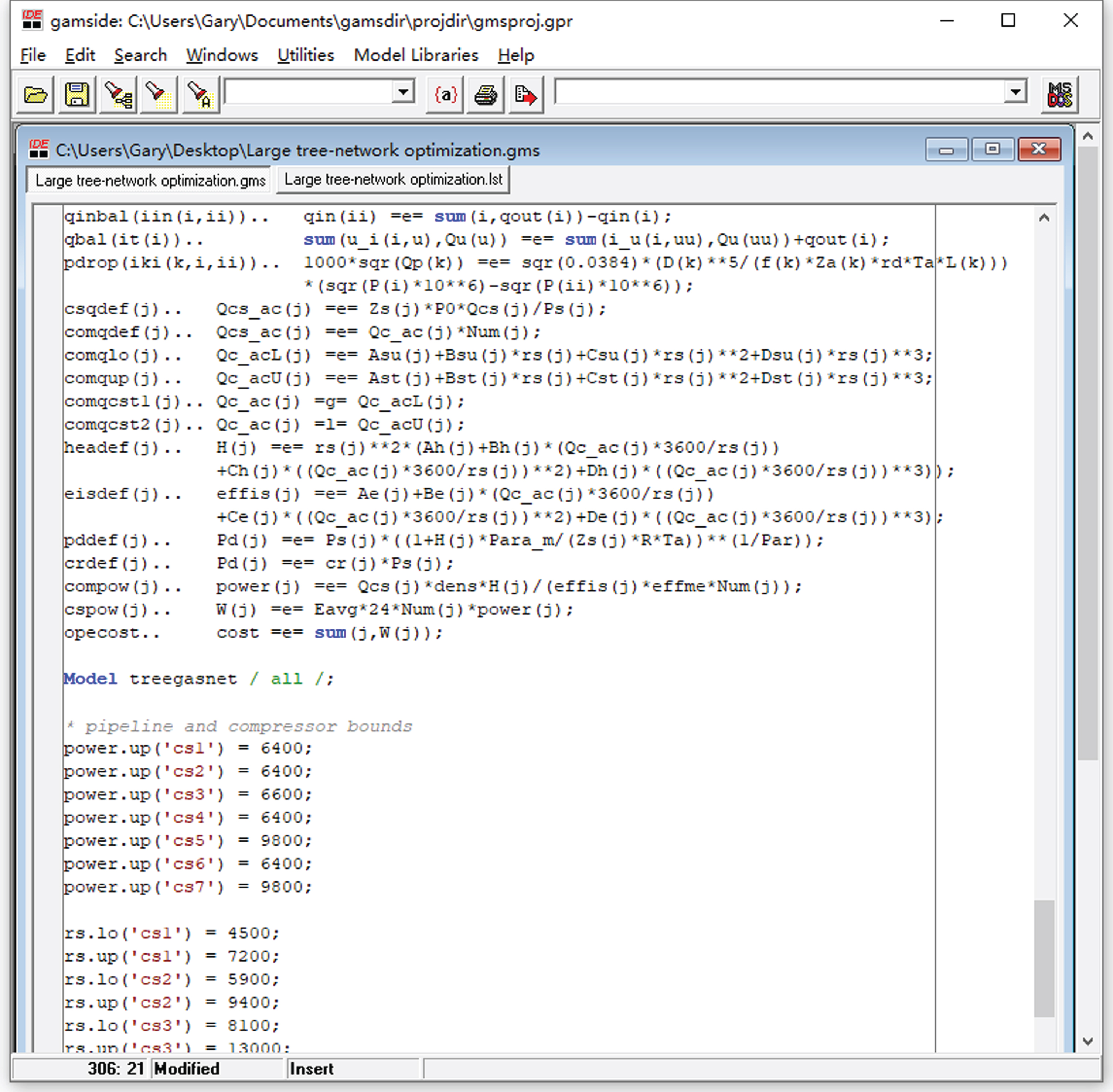
Basic part of modeling along with coding according to GAMS.

4 Case study

A practical large tree-topology gas transmission network is selected as a study example. The total length of this network is 2229 km, and it contains 1 trunk pipeline, 3 branch pipelines, 2 GINs, 20 GDNs, and 7 CSs. The schematic diagram of the network is shown in Fig. 6. The design operating pressure of the network is 10 MPa. The internal diameter is 981 mm, the wall thickness is 17.5 mm, and the absolute roughness of the pipe’s internal wall is 0.01 mm.

Fig. 6

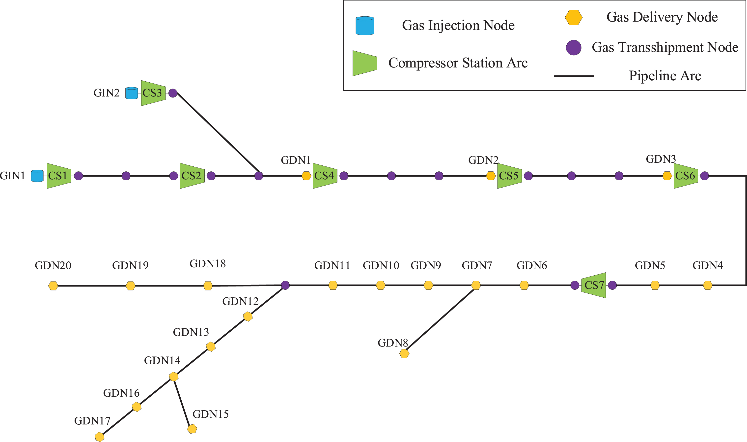
Schematic of a large tree-topology gas transmission network.

The maximum power of a single compressor of the seven compressor stations is divided into three levels of 6400 kW, 6600 kW and 9800 kW. All compressors are driven by electric motors. The configuration parameters of each compressor station are shown in Table 1. Different compressor stations are completed at different times and have different self-pressurizing capabilities. Therefore, the compressor characteristics of the compressor station are also different. The coefficients in the compressor head characteristic equation and efficiency characteristic equation of each compressor station are explained in detail (Tables 2 and 3), respectively. All coefficients are determined by nonlinear least squares regression. In addition, the average power price of CSs in this network is 0.52983¥/(kW·h), which is calculated based on the production operation report of the network operating company in 2019.

Table 1

Configuration parameters of different CSs

No.	Device driver	Maximum compressor power	Arrangement
CS 1	Motor	6400 kW	2 + 1
CS 2	Motor	6400 kW	2 + 1
CS 3	Motor	6600 kW	3 + 1
CS 4	Motor	6400 kW	3 + 1
CS 5	Motor	9800 kW	2 + 1
CS 6	Motor	6400 kW	3 + 1
CS 7	Motor	9800 kW	2 + 1

Table 2

Head characteristic equation coefficients of different CSs

No.	A_H	B_H	C_H	D_H
CS 1	0.0000000943	0.0000026463	–0.0000021481	0.0000004607
CS 2	0.0000003569	0.0000009399	–0.0000011022	0.0000002623
CS 3	0.0000000782	0.0000080441	–0.000021477	0.0000154818
CS 4	0.0000000844	0.0000026628	–0.0000021519	0.0000004599
CS 5	0.0000004769	0.0000008023	–0.0000005996	0.0000000876
CS 6	0.0000001078	0.000002598	–0.0000020893	0.0000004413
CS 7	0.0000004761	0.0000008054	–0.0000006028	0.0000000886

Table 3

Efficiency characteristic equation coefficients of different CSs

No.	A_e	B_e	C_e	D_e
CS 1	0.657763	0.384167	–0.152314	–0.013504
CS 2	0.450659	0.707019	–0.025386	–0.266559
CS 3	0.547286	0.674449	2.237476	–5.486256
CS 4	0.670613	0.353805	–0.128931	–0.019123
CS 5	0.493605	0.356031	0.079847	–0.098892
CS 6	0.704779	0.270288	–0.061935	–0.036387
CS 7	0.493605	0.356031	0.079847	–0.098892

An actual operation scheme of the network is selected as the comparison scheme of optimization results. Under this practical scheme, the network total transmitting volume is 3142.85×10⁴m³/d, and the flow rate distribution of each GIN and GDN in the network is shown in Fig. 7. At the first GIN, natural gas with a constant flow of 2445.72×10⁴m³/d is injected into the pipeline with a pressure of 7.45 MPa, while at the second GIN, 697.14×10⁴ m³/d natural gas is injected into the pipeline with a pressure of 3.8 MPa. It should be noted that the outlet pressure of GDN 15 must be greater than 4.8 MPa, and the pressure at the GDN 20 must be greater than 5.2 MPa. In addition, the average composition of natural gas in the network is shown in Table 4. Then, some basic parameters including compressibility factor, density, relative density and friction factor can be calculate by the BWRS state equation and Colebrook equation.

Fig. 7

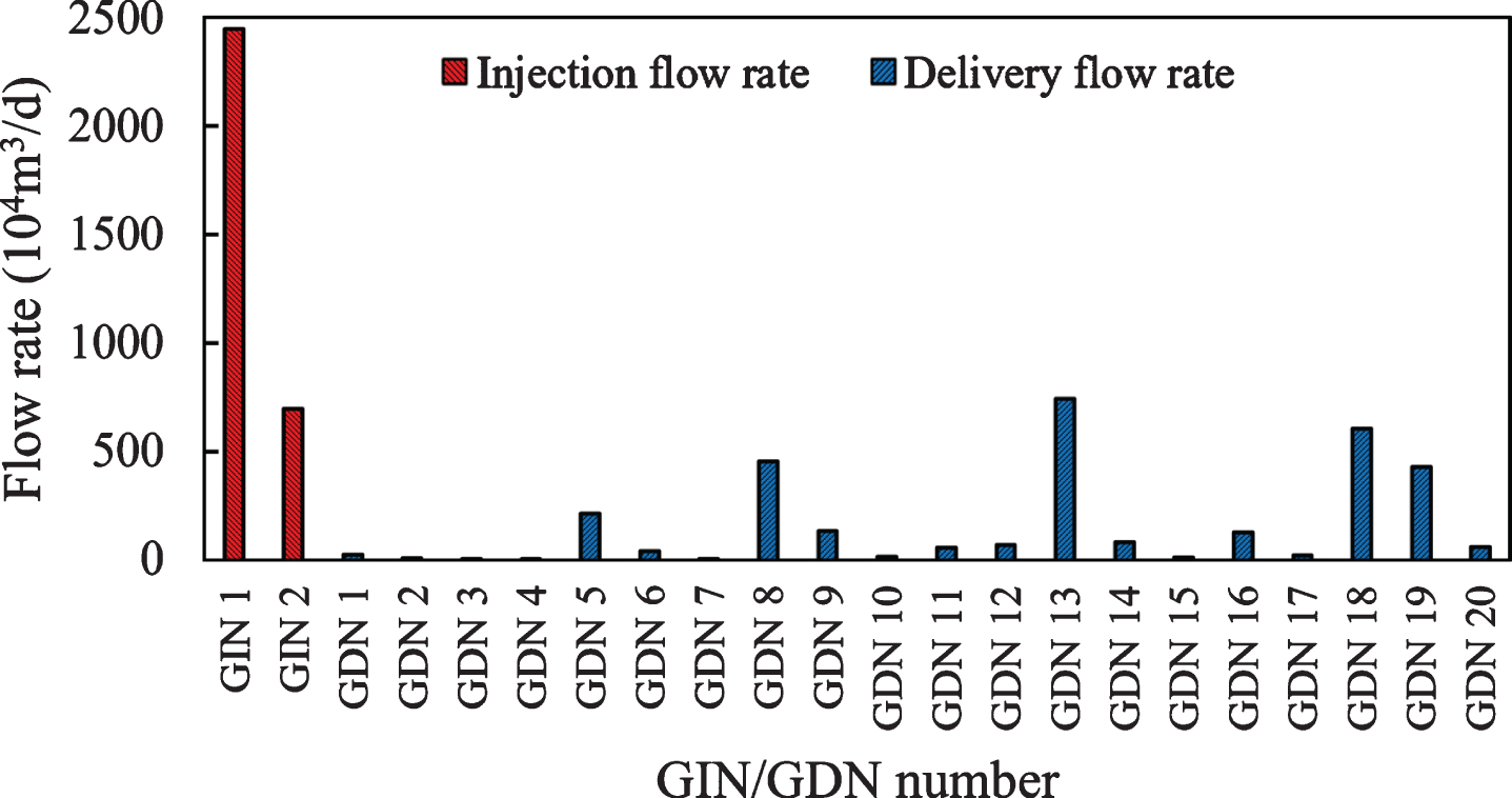
Flow rate distribution of each GIN and GDN.

Table 4

Natural gas composition

Component	CH₄	C₂H₆	He	N₂	CO₂
Mole fraction (%)	97.16	0.04	0.02	0.91	0.91

Now, we assume that due to the adjustment of energy structure and policy orientation of the region where GDN 19 is located, natural gas demand in the region would increase significantly. Therefore, on the premise of ensuring the safe and stable operation of the system, it is necessary to increase the gas transmission capacity of this node as much as possible to meet the regional gas consumption demand. All the added natural gas is provided by GIN 2. Based on this, our multi-objective function is adjusted to GDN 19 delivery flow rate maximization and CS power consumption cost minimization. Hence, the following questions through solving such multi-objective optimization problems can be better answered: (1) If there is a upper bound on the energy cost of the compressor station of this system, how to determine the maximum delivery flow rate at GDN 19 by adjusting the operating parameters; (2) How to adjust the operating parameters to achieve the minimum energy cost of the compressor station under the condition of meeting the delivery flow rate at GDN 19.

In addition, there are some constraints at GDNs and CSs to control the changes in decision variables in terms of the operating requirements of natural gas networks. The change range of delivery flow rate at GDN 19 is 428.57–950×10⁴m³/d. The other variation range of each decision variable is shown in Table 5. For the number of RCs, the range of CS 3, CS 4 and CS 6 is 0–3, and the other CSs is 0–2. As for the range of change in compressor speed, the range of CS 1, CS 4 and CS 6 is 4500–7200 r/min, while CS 2 of that is 5900–9400 r/min, and CS 3 has the highest compressor rotational speed within 8100–13000 r/min. Moreover, delivery pressure at the GDN15 and GDN 20 must be greater than 4.8 MPa and 5 MPa, respectively. The discharge pressure of each compressor station needs to be controlled within 9.85 MPa to guarantee the safe and stable operation of the pipeline system.

Table 5

Variation range of each decision variable

Bounds	Number of RCs							Rotating speed (r/min)
	δ ₁	δ ₂	δ ₃	δ ₄	δ ₅	δ ₆	δ ₇	ω ₁	ω ₂	ω ₃	ω ₄	ω ₅	ω ₆	ω ₇
Lower bounds	0	0	0	0	0	0	0	4500	5900	8100	4500	5700	4500	5700
Upper bounds	2	2	3	3	2	3	2	7200	9400	13000	7200	9000	7200	9000

5 Results and discussions

5.1 Optimization results

In the above study, we established a multi-objective optimization model involving two optimization goals (maximizing the specific GDN delivery flow rate and minimizing the energy cost of CSs). The ɛ-constraint method and GAMS/ DICOPT solver were adopted to solve the model. A large practical tree-topology gas transmission network is investigated as an optimization example. During the solution process, the initial value range of ɛ_u is 428.57–950×10⁴m³/d, and the step size is 4.32×10⁴m³/d. However, once ɛ_u exceeds 921.05×10⁴m³/d, no feasible solution can be obtained. This is because the pressure drop increases as the flow increases after delivery flow rate at GDN19 exceeds 921.05×10⁴m³/d. Even if the last CS provides the maximum outbound pressure of 9.85 MPa, it could not meet the requirement that the pressure at GDN15 is not less than 4.8 MPa. Therefore, the value range of ɛ_u is adjusted to 428.57–921.05×10⁴m³/d, and the ɛ-constraint method finally solves 115 single-objective problems.

The Pareto front calculation results of the two-objective optimization problem proposed in this paper are calculated and demonstrated (Fig. 8). Each dot on the Pareto front represents a Pareto optimal solution. It can be seen from the figure that the power consumption of the CS increases with the increase of the delivery flow rate at GDN 19. This tells that the two optimization goals are in conflict with each other and cannot be achieved the optimum value at the same time. As the flow rate increases, the growth rate of compressor energy consumption also gradually accelerates. Points A, B, and C in Fig. 8 represent the Pareto optimal solutions under the conditions of minimum, medium, and maximum GDN19 delivery flow rate respectively. Then this article will use these three points as examples to discuss the differences between different Pareto optimal solutions. Besides, it can be seen from Fig. 8 that the function value of the optimal solution set (Pareto front) of the optimization problem is located at the lower boundary line of the entire objective function space. In the entire feasible region, all feasible solutions except the Pareto front are dominated by the solutions on the Pareto front. Domination means that in the two solutions compared with each other, all the objective functions of one solution are not worse than the other solution, and at least one objective function is better than the other solution. Take the points X1, X2, and X3 in Fig. 2 as an example. Point X1 is located in the feasible region but is not optimal. This point is dominated by points X2 and X3 on the Pareto front. That is, when the flow is the same, the energy consumption of the compressor station at X2 is lower than X1. When the energy consumption is the same, the flow rate delivered by point X3 is higher than that of X1. Therefore, the solution on the Pareto front has the least conflict of goals compared with other solutions, and can provide a better choice for decision-makers.

Fig. 8

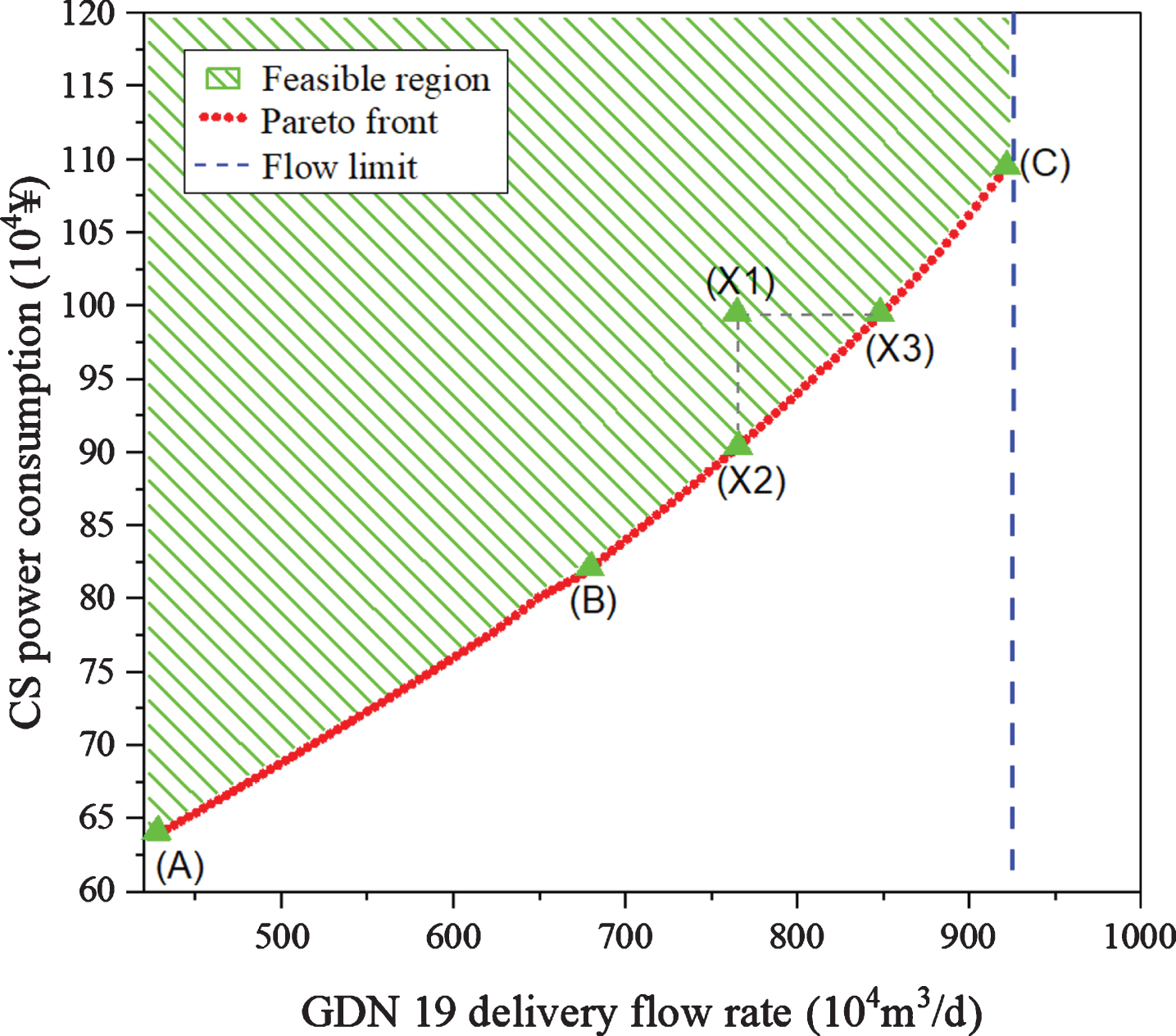
Pareto front for bi-objective optimization of the gas transmission network.

5.1.1 Comparison between Pareto optimal solution and actual operation scheme

First, point A in the Pareto front is selected to compare with the actual operation scheme in order to analyze the feasibility and optimization effect of the optimization result. Point A is the point where the power cost of the CS is the smallest in the Pareto front (Fig. 8), while the GDN 19 delivery flow rate at this point is exactly the same as the actual operation scheme. Therefore, the case of point A has a pipeline flow situation that is completely consistent with the actual operation scheme, which can be used to represent the effect of the optimization results. The power consumption cost of CSs in the actual operation scheme is 70.94×10⁴ ¥, while the optimization result is 63.99×10⁴ ¥. By comparing the optimization result of point A with the actual power consumption cost of CSs, the optimization result saves a power consumption cost of 9.79%.

We compared the number of RCs between the optimization results and the actual operation scheme (Fig. 9(a)). It can be seen from the figure that, except for the CS 1, the RCs number in each CS is the same in both schemes. The RCs number in CS 1 is one in the actual operation scheme while two in the optimization result. One more compressor runs in the optimization result than the actual operation scheme. Besides, the comparison between the optimization results and the actual CS rotating speed in each station is shown in Fig. 9(b). It can be seen from the figure that only in CS 3, the rotating speed in the optimization results is higher than the actual operation scheme. As for other CSs, the rotating speed in the optimization results is lower than the actual operation scheme. Besides, the comparison of each CS total power is illustrated, as shown in Fig. 9(c). It is observed that the power of CS 1 and CS 3 in the optimization result is higher than the actual operation scheme. But the power of CS 2, CS 4, CS 5, CS 6 and CS 7 in the optimization result is lower than the actual operation scheme, especially the CS 5. Obviously, optimization strategy of the optimization result is to increase the power of the upstream compressor station and reduce the power of the downstream compressor station. This is also the reason why the RCs number in CS 1 of optimization result is increased. Next, we will further analyze this optimization strategy by pipeline pressure drop.

Fig. 9

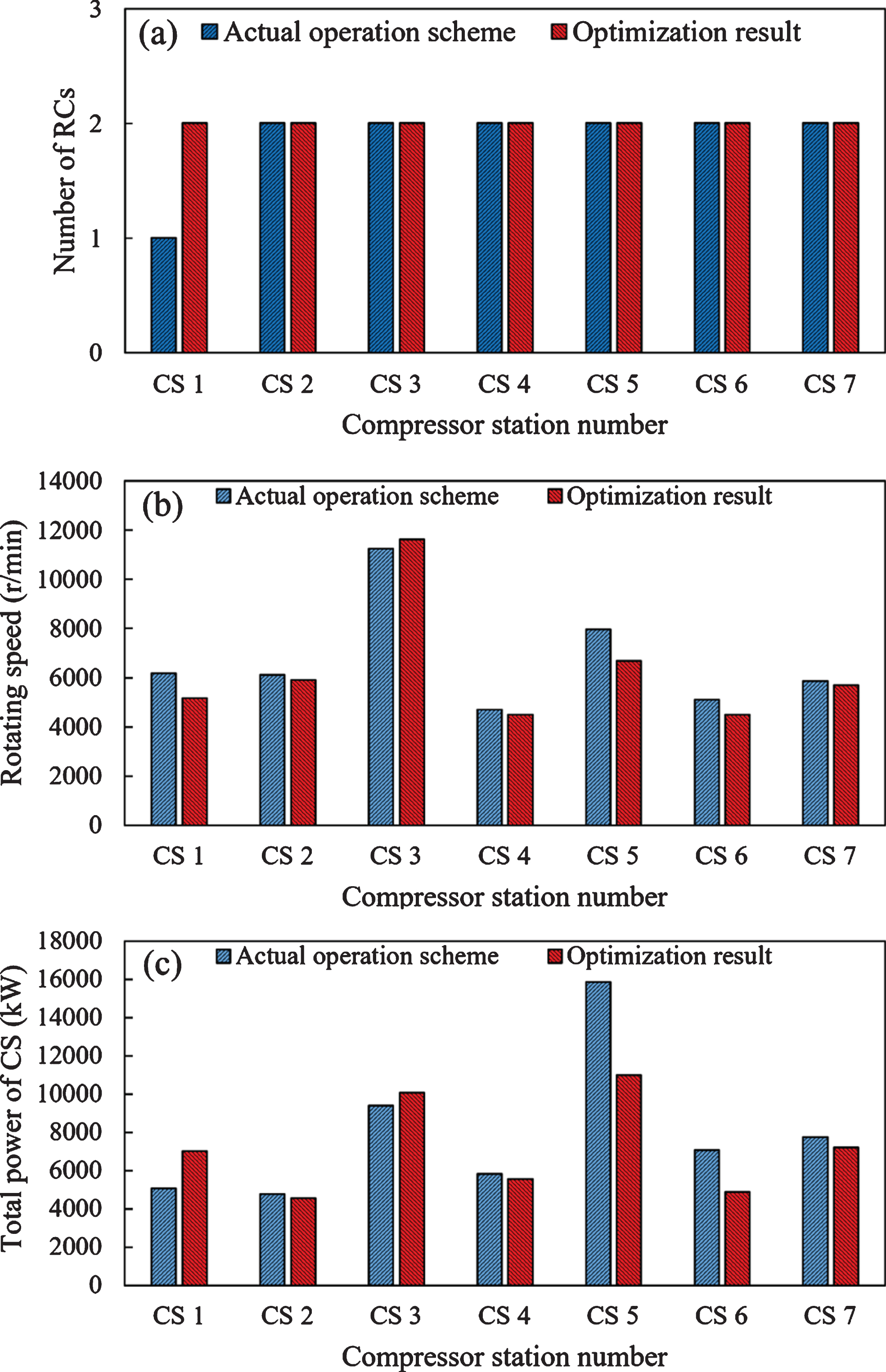
Comparison between the optimized results and the actual operation scheme: (a) running compressor number; (b) compressor rotating speed; (c) CS total power.

The comparison of the trunk pipeline pressure drop between the optimization result and the actual operation scheme is shown in Fig. 10. The following conclusions can be drawn through analyzing the figure. In the optimization result, the discharge pressure of CS 1, CS 2, CS 4 and CS 5 are higher than the actual operation scheme, the discharge pressure of CS 6 is almost equal to the actual operation scheme, but the CS 7 discharge pressure is lower than the actual one. It is worth noting that, as the discharge pressure of the upstream 4 CSs in the optimization results increased, the suction pressure of the adjacent CSs also increased, thus reducing the boost degree of this adjacent compressor stations to some extent. This phenomenon is more obvious in CS 5 and CS 6. Combined with Fig. 10(c) above, it can be seen that the reduction of the boost degree of this two CSs save a lot of power consumption for the optimization results. This is also the main reason why the optimization result is better than the actual operation scheme. In addition, the comparison between the optimization results and the actual terminal pressure of each pipeline is shown in Fig. 11.

Fig. 10

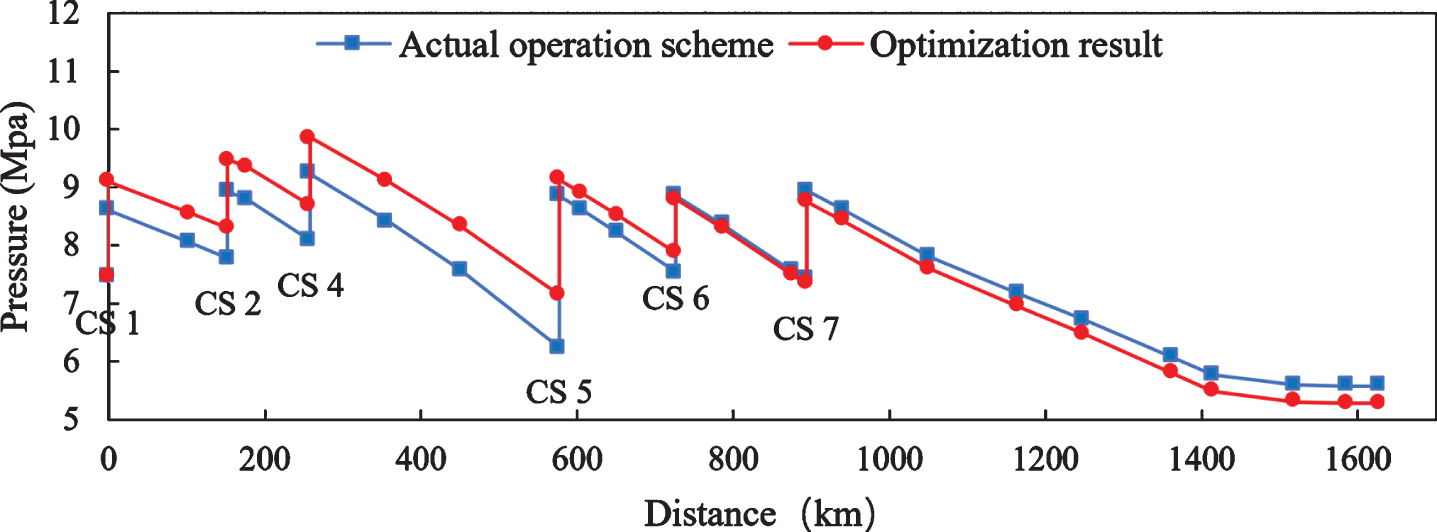
Comparison of trunk pipeline pressure drop.

Fig. 11

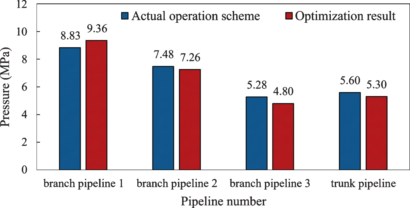
Comparison of pipeline terminal pressure.

It can be seen from the figure that at the branch 3, optimized end-point pressure of the pipeline is just the minimum allowable pressure of 4.8 MPa, which just meets the minimum pressure constraint of the gas point. However, the end pressure of branch 3 of the actual operation scheme is 5.28 MPa and obviously there is a waste of energy. This is another reason that optimization results are more economical.

5.1.2 Comparison between different pareto optimal solutions

The next stage is to analyze the difference between the optimization results of different Pareto optimal solutions. Three representative points are selected for analysis from the Pareto front, including points A, B, and C (Fig. 8). The objective function values at points A-C are shown in Table 6. As we can be seen from the table: (1) Case of point A has the lowest delivery flow rate at GDN 19 and the power cost of the CS; (2) Case of point C has the highest delivery flow rate at GDN 19 and the power cost of the CS; (3) The two objective function values of point B are between points A and C. Besides, Fig. 12(a) shows the number of RCs at points A to C. The difference mainly occurs at CS 3 and CS 6, of which the number of RCs in case of point A are two, 3 and 2 respectively of CS 6 in case of B, and all 3 in case of C. The compressor rotating speed of each station at points A-C is shown in Fig. 12(b). The differences mainly appear in CS 5, CS 6 and CS 7.

Table 6
Optimization results of objective functions for Points A-C

Objective functions Optimization results

Point A Point B Point C

Delivery flow rate at GDN 19 (10⁴m³/d) 428.57 679.13 921.05

CS power consumption cost (10⁴¥) 63.99 82.10 109.45

Objective functions	Optimization results
Delivery flow rate at GDN 19 (10⁴m³/d)	428.57	679.13	921.05
CS power consumption cost (10⁴¥)	63.99	82.10	109.45

Fig. 12

Points A-C: (a) number of RCs; (b) compressor rotating speed.

5.1.3 Analysis of decision variables variation with pareto front

We analyzed the changes in the number of RCs at each station and in the speed with the Pareto front to further find out the detailed change trend and key change points of the decision variables of the Pareto front. The results are shown in Figs. 13 and 14. Specifically, the dashed lines in the figure represent the upper or lower limits of the variable, respectively. Figure 13(a) and (b) show the changes of δ₃ and δ₆ in the Pareto front, respectively. Since the number of RCs of other CSs has always remained the same, they are not discussed. It can be seen from Fig. 13(a), δ₃ is 2 at the point where delivery flow rate of GDN 19 is 653.21×10⁴m³/d. After reaching this point, δ₃ becomes 3. As can be seen from Fig. 13(b), it is initially used for 2 compressors, and maintains a large flow rate range, and it becomes 3 until the distribution flow rate reaches 813.05×10⁴m³/d.

Fig. 13

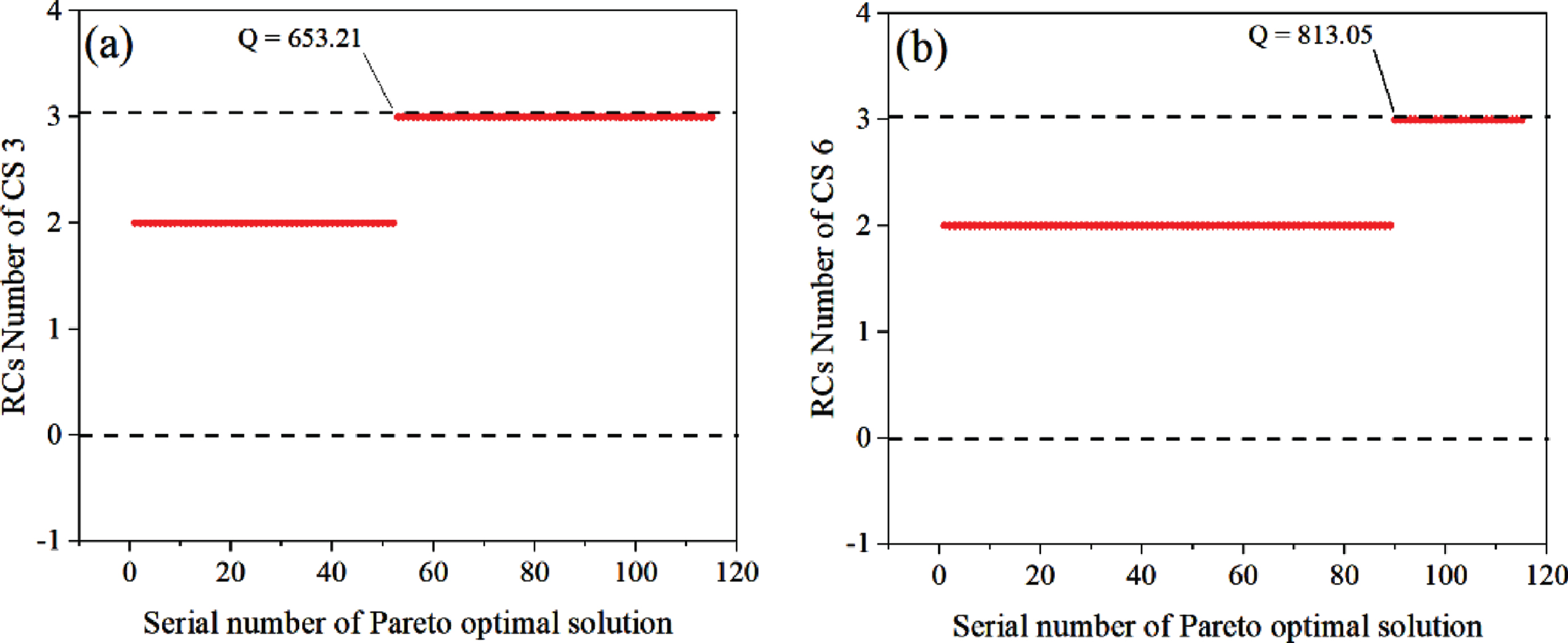
Change of running compressors number with the Pareto optimal solution: (a) CS 3; (b) CS 6.

The change of the compressor rotating speed at the Pareto front of each of the seven CSs is shown in Fig. 14. As shown in Fig. 14(a), it grows slowly first, then undergoes a process of rapid decrease and rise, and finally maintains slow growth. It can be seen from Fig. 14(b) that the lower bound is 5900 r/min at all points. So, the changes in flow have little effect on ω₂. As shown in Fig. 14(c), ω₃ is maintained at a high level, and gradually increases first, and then a small decrease occurs at GDN19 at a gas flow rate of 627.29×10⁴m³/d. This is because the power of a single compressor of CS 3 has reached the upper limit of 6600 kW at this point. ω₃ must be reduced in order to meet the power constraint. Then, at the point where the distribution flow is 653.21×10⁴m³/d, ω₃ shows a significant decrease. The reason is that at this point, the number of compressor start-ups of CS 3 became three, and the inlet flow rate of a single compressor decreases, and the speed also decreases accordingly. ω₃ (Fig. 14(d)) keeps increasing after that. It is noted that ω₄ is maintained at the lower limit of the speed at first, followed by a process of rapid rise and then decline occurs, and finally maintains at the lower limit. ω₅ (Fig. 14(e) increases sharply at the beginning, but suddenly stops growing at a point of 679.13×10⁴m³/d, and then keep fluctuating within a small range. This is because that at a point of 679.13×10⁴m³/d, the single compressor power of CS 5 has reached the upper limit of 9800 kW, and no more compressors can be put into use at this station. As shown in Fig. 14(f), ω₆ initially maintains the lower limit, and it does not start to increase significantly until the distribution flow is 679.13×10⁴m³/d. However, at the point where the distribution flow is 813.05×10⁴m³/d, ω₆ suddenly drops, and then continues to increase. This is because the number of start-ups in CS 6 has changed to three at this point, the inlet flow rate of a single compressor has been greatly reduced, and the speed has been greatly reduced. The change of ω₇ is shown in Fig. 14(g). It can be seen from the figure that ω₇ maintains the lower limit of the rotating speed from the beginning. It does not start to rise until the flow is 856.25×10⁴m³/d.

Fig. 14

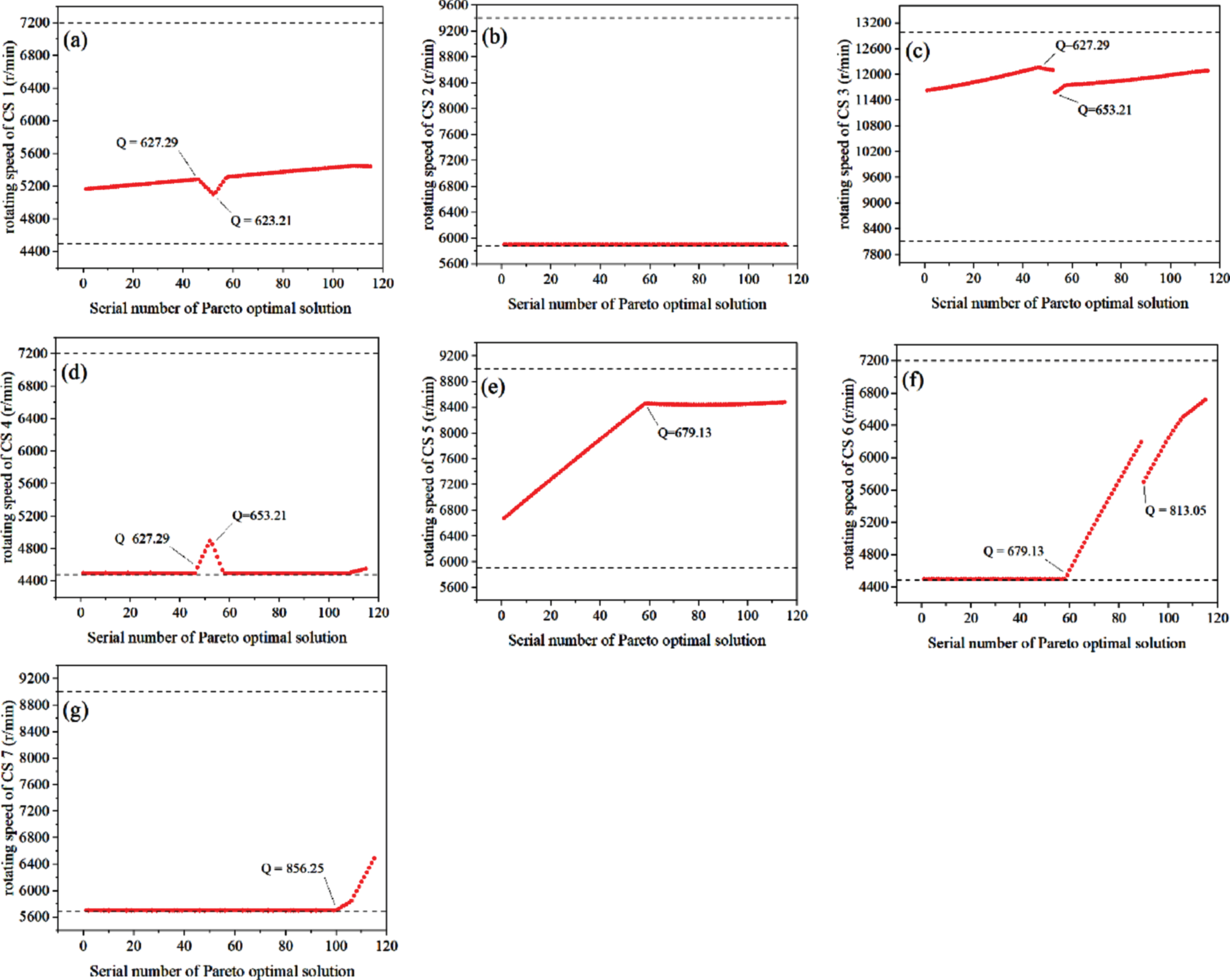
Change of compressor rotating speed with the Pareto optimal solution: (a) CS 1; (b) CS 2; (c) CS 3; (d) CS 4; (e) CS 5; (f) CS 6; (g) CS 7.

Through the above analysis, it can be found that the key points of each decision variable’s change with the Pareto front point are the same in some CSs. This is because at these key points the number of start-ups has changed, or the power of a single unit has reached the upper limit, resulting in varying of decision variables for CSs along the pipe. Therefore, the various decision variables affect each other and ultimately affect the optimization result in the optimization process. In addition, the solution of this optimization problem includes 15 decision variables, and the decision space where the solution vector is located is a 15-dimensional vector space. According to the previous analysis of the change of decision variables in the Pareto optimal solution, we can see that among all decision variables, the values of 5 decision variables including δ₁, δ₂, δ₅, δ₇, ω₂ are always boundary values. The variable value of the running compressors number δ₁, δ₂, δ₅, δ₇ is always the upper boundary value of 2, and the compressor speed variable ω₂ is always the lower boundary value of 5900 r/min. Therefore, the solution vectors in the Pareto optimal solution set are all on the boundary of the original decision space, and the resulting solution space is the boundary subspace of the original decision space.

In general, every point on the Pareto front is a feasible solution. The final optimal solution can be selected from the Parato front via a process of decision-making. In the natural gas industry, decision makers are one or a group people who have a better understanding of the network operation and the relevant costs. During the decision-making process, operators can use practical information and experience to select the best operational scheme, to satisfy contract gas delivery requirement with the lowest economic cost.

5.2 Sensitivity analysis

The optimization results are the results of the joint action of multiple operating parameters. Consequently, we performed a sensitivity analysis in order to know the impact of each operating parameter changes on the optimization results. Sensitivity analysis is carried out for pipeline parameters and compressor parameters, respectively. As a result, we can better predict and understand the optimization results.

The section mainly analyzes the effect of inlet flow rate and inlet pressure changes on the pressure drop of the pipeline. A section of natural gas pipeline with an inner diameter of 1016 mm and length of 125.6 km is selected for analysis. The range of values for each parameter for sensitivity analysis is shown in Table 7. The analysis results are obtained through simulation of the previously established pipeline and compressor station models. It can be seen from the figure (Fig. 15(a)) that as the flow increases, the pressure drop also continues to increase, and there is a non-linear relationship between the two. The influence of the inlet pressure changes on the pressure drop is shown in Fig. 15(b). It can be seen from the figure that as the pressure of the pipeline inlet increases, the pressure drop of the pipeline continuously decreases. Therefore, maintaining the pressure of the entire pipeline at a high level can reduce the pressure drop and save system energy consumption.

Table 7
Variation range of flow rate and inlet pressure

Inlet pressure (MPa) Inlet flow rate (10⁴m³/d) Results

7.57 2000–3670 Fig. 15(a)

5.6–7.57 3670 Fig. 15(b)

Inlet pressure (MPa)	Inlet flow rate (10⁴m³/d)	Results
7.57	2000–3670	Fig. 15(a)
5.6–7.57	3670	Fig. 15(b)

Fig. 15

Effects of various parameters of the pipeline on the pressure drop: (a) flow rate; (b) inlet pressure.

Coming to the next is the sensitivity analysis of compressor station parameters. This section mainly analyzes the impact of changes in compressor intake gas flow rate, speed and suction pressure on discharge pressure and energy consumption costs. The influence of each parameter, considering the upper and lower bounds of the parameters for different compressor startups, is represented in Fig. 16. A compressor station in the calculation example is selected for analysis in the process analysis. The ranges of the three parameters are shown in Table 8.

Fig. 16

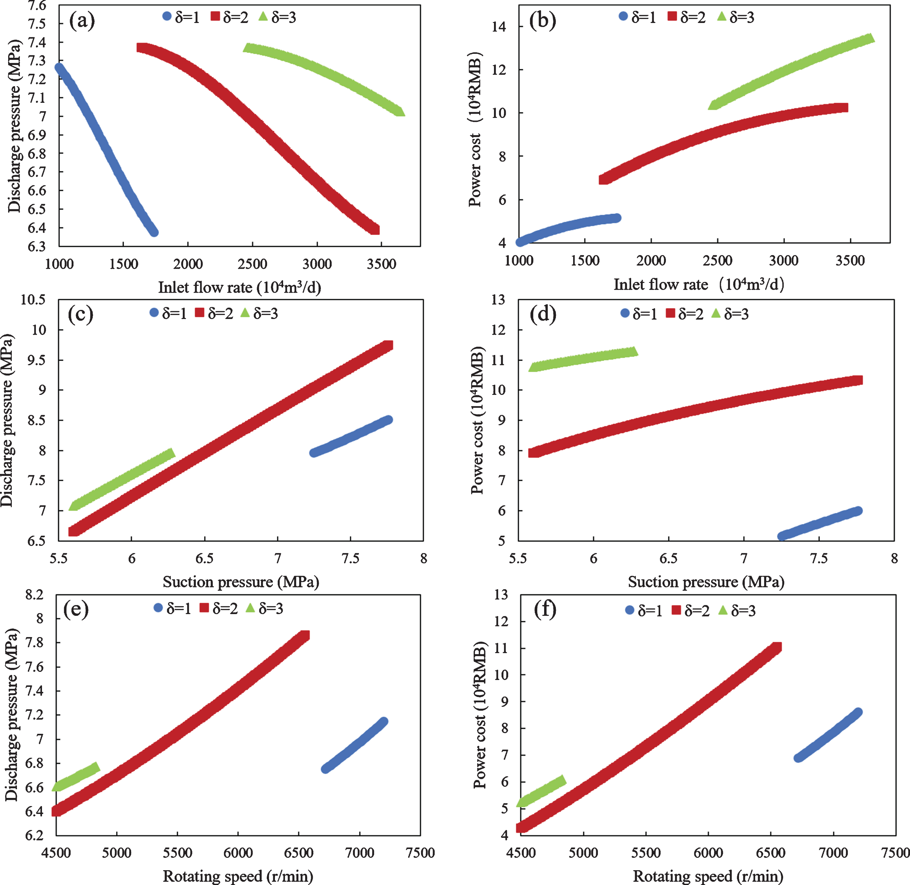
Impact of parameters on compressor performance under different running compressor numbers: (a) inlet flow rate vs. discharge pressure; (b) inlet flow rate vs. energy costs; (c) suction pressure vs. discharge pressure; (d) suction pressure vs. energy costs; (e) rotating speed vs. discharge pressure; (f) rotating speed vs. energy costs.

Table 8

Variation range of suction pressure, rotating speed and inlet flow rate

Suction pressure (MPa)	Rotating speed (r/min)	Inlet flow rate (10⁴m³/d)	Results
5.6	5850	1000∼3650	Fig. 16(a) and 16(b)
5.6∼7.76	5450	2550	Fig. 16(c) and 16(d)
5.6	4500∼7200	1900	Fig. 16(e) and 16(f)

Figure 16(a) and (b) demonstrate the influence of inlet gas flow rate on discharge pressure and energy cost. As shown in Fig. 16(a), as the inlet gas flow rate increases, the discharge pressure decreases continuously. Besides, the increase of the inlet gas flow rates also leads to an increase in the energy cost of the compressor (Fig. 16(b)), which means that more compressors are needed to meet the increase of inlet flow rate. At the same inlet flow rate, increasing the number of RCs would increase the discharge pressure, causing more energy costs. The relationship between compressor suction pressure, discharge pressure and energy cost is displayed by Fig. 16(c) and (d). As shown in the figure, an increase in suction pressure leads to an increase in discharge pressure and energy costs. Further, at the same suction pressure, an increase in the number of RCs has resulted in an increase in discharge pressure and energy costs. But the increase in energy costs is higher than the discharge pressure. The relationship between rotating speed, discharge pressure and energy costs are shown in Fig. 16(e) and (f). As shown in Fig. 16(e), increasing the compressor’s rotating speed can cause higher discharge pressure. But higher rotational speeds also mean higher energy costs (Fig. 16(f)).

In summary, higher compressor discharge pressure can be obtained by increasing the compressor’s suction pressure, rotating speed, number of RCs or reducing the inlet flow. However, compressor suction pressure and inlet gas flow rate are mainly affected by the inlet natural gas conditions and the operation of upstream units. From the perspective of compressor station variables, it is possible to consider increasing the number of RCs or the rotating speed. In addition, an increase in the discharge pressure of a compressor station would also lead to an increase in the suction pressure of the downstream compressor station, thus increasing the discharge pressure of the downstream compressor station accordingly. But increasing the number of RCs or the rotating speed inevitably leads to an increase in the energy cost of the compressor station. Therefore, an optimization method must be applied to balance the influence between various parameters to achieve the optimal system operating conditions.

6 Conclusion

This paper studied the technical and economic operation optimization of natural gas transmission network to balance two conflicting optimization objectives (i.e. maximum delivery flow rate of a specified GDN and minimum CS power consumption cost). The established optimization model is applied to a large tree-topology gas network. Then, the ɛ-constraint method was adopted to transform the bi-objective optimization model into 115 single-objective optimization models, and these single-objective models were solved on the GAMS optimization platform, which took 34.385 s. A set of Pareto optimal solutions is obtained for multi-objective optimization, that is, a trade-off solution between two conflicting objective functions. Besides, a sensitivity analysis is performed in order to understand the influence of changes in operating parameters on the optimization results. The following conclusions can be drawn from the analysis of the optimization results: the CS power consumption cost increases with the increase of the delivery flow rate at GDN 19, and the growth rate increases gradually; the maximum flow rate that the network system can provide to the GDN 19 is 921.05×10⁴ m³/d; The optimization results save 9.79% of operating costs compared to the actual operation plan, which proved the validity of proposed method; With the increase of the delivery flow rate at GDN 19, the number of RCs of CS 3 and CS 6 change from 2 to 3 with the delivery flow rate of 653.21×10⁴m³/d and 813.05×10⁴m³/d respectively; The single compressor power of CS 5 reaches the upper limit of 9800 kW at 679.13×10⁴m³/d, and has maintained this upper limit. In the process of making gas network operation plan, the number of compressor starting and the running power are also important references. Finally, operators can choose a final pipeline operation scheme from the Pareto optimal solution according to the demands and actual conditions. In the future, researchers should consider on the basis of economic goals, continue to introduce safety, reliability or other goals into the multi-objective operation optimization of gas pipelines, so that the optimization scheme can be further complete and comprehensive.

Conflict of interests

The authors declare that there is no conflict of interests regarding the publication of this paper.

Statement of data availability

All data, models, and code generated or used during the study appear in the submitted article.

Footnotes

Acknowledgments

This work was part of the program “Study on the optimization method and architecture of oil and gas pipeline network design in discrete space and network space”, funded by the National Natural Science Foundation of China, grant number 51704253. The authors are grateful to all study participants.

References

Ríos-Mercado

R.Z.

and Borraz-Sánchez

, Optimization problems in natural gas transportation systems: A state-of-the-art review[J], Applied Energy 147 (2015), 536–555.

Zhou

, Zhou

, Liang

G.C.

and Peng

J.H.

, An MINLP model for network layout of underground natural gas storage[J], Journal Of Intelligent & Fuzzy Systems 38(4) (2020), 4619–4642.

Wei

L.X.

, Dong

, Zhao

and Zhou

, Optimization model establishment and optimization software development of gas field gathering and transmission pipeline network system[J], Journal Of Intelligent & Fuzzy Systems 31(4) (2016), 2375–2382.

Liu

E.B.

, Lv

L.X.

, Ma

and Zhang

, Steady-state optimization operation of the west–east gas pipeline[J], Advances in Mechanical Engineering 11(1) (2019), 1–14.

IEA. World Energy Outlook 2018[R].

BP. BP Energy Outlook: 2019 edition. 2019[R]. London, UK.

Tabkhi

, Optimization of gas transmission networks[D], Institut National Polytechnique De Toulouse (2007).

, Li

C.J.

, He

Y.F.

and Jia

W.L.

, Operation optimization of natural gas transmission pipelines based on stochastic optimization algorithms: A Review[J], Mathematical Problems in Engineering 2018 (2018), 1–18.

Pfetsch

M.E.

, Fügenschuh

, Geißler

, et al., Validation of nominations in gas network optimization: models, methods, and solutions[J], Optimization Methods and Software 30(1) (2015), 15–53.

10.

Farahani

and Rezapour

, Logistics operations and management: concepts and models[M], Elsevier (2011).

11.

Wong

P.J.

and Larson

R.E.

, Optimization of natural-gas pipeline systems via dynamic programming[J], IEEE Transactions on Automatic Control 13(5) (1968), 475–481.

12.

Percell

P.B.

and Ryan

M.J.

, Steady state optimization of gas pipeline network operation[C], In: 19th PSIG Annual Meeting, (1987).

13.

Wolf

D.D.

and Smeers

, The gas transmission problem solved by an extension of the simplex algorithm[J], Management Science 46(11) (2000), 1454–1465.

14.

Arya

and Honwad

, Modeling, Simulation, and Optimization of a High-Pressure Cross-Country Natural Gas Pipeline: Application of an Ant Colony Optimization Technique[J], Journal Of Pipeline Systems Engineering And Practice 7(1) (2016).

15.

Mohamadibaghmolaei

, Mahmoudy

, Jafari

, Mohamadibaghmolaei

and Tabkhi

, Assessing and optimization of pipeline system performance using intelligent systems[J], Journal of Natural Gas Science & Engineering 18 (2014), 64–76.

16.

Zhang

Z.W.

and Liu

X.T.

, Study on optimal operation of natural gas pipeline network based on improved genetic algorithm[J], Advances in Mechanical Engineering 9(8) (2017).

17.

Rodrguez

D.A.

, Oteiza

P.P.

and Brignole

N.B.

, Simulated annealing optimization for hydrocarbon pipeline networks[J], Industrial & Engineering Chemistry Research 52(25) (2013), 8579–8588.

18.

Khanmirza

, Madoliat

and Pourfard

, Transient Optimization of Natural Gas Networks Using Intelligent Algorithms[J], Journal Of Energy Resources Technology-Transactions Of The ASME 141(3) (2019).

19.

Tran

T.H.

, French

, Ashman

and Kent

, Linepack planning models for gas transmission network under uncertainty[J], European Journal Of Operational Research 268(2) (2018), 688–702.

20.

Kazda

, Tomasgard

, Norstebo

and Li

, Optimal utilization of natural gas pipeline storage capacity under future supply uncertainty[J], Computers & Chemical Engineering (2020), 139.

21.

Zhang

X.R.

, Wu

C.C.

and Zuo

L.L.

, Minimizing fuel consumption of a gas pipeline in transient states by dynamic programming[J], Journal Of Natural Gas Science And Engineering 28 (2016), 193–203.

22.

Kazda

and Li

, Approximating Nonlinear Relationships for Optimal Operation of Natural Gas Transport Networks[J], Processes 6(10) (2018).

23.

Uster

and Dilaveroglu

, Optimization for design and operation of natural gas transmission networks[J], Applied Energy 133 (2014), 56–69.

24.

, Li

C.J.

, Jia

W.L.

and He

Y.F.

, Optimal operation of trunk natural gas pipelines via an inertia-adaptive particle swarm optimization algorithm[J], Journal of Natural Gas Science and Engineering 21 (2014), 10–18.

25.

Alinia Kashani

A.H.

and Molaei

, Techno-economical and environmental optimization of natural gas network operation[J], Chemical Engineering Research and Design 92(11) (2014), 2106–2122.

26.

Demissie

, Zhu

W.H.

and Belachew

C.T.

, A multi-objective optimization model for gas pipeline operations[J], Computers and Chemical Engineering 100 (2017), 94–103.

27.

, Zio

, Zhang

J.J.

, Li

X.Y.

, Chi

L.X.

, Fan

and Zhang

Z.J.

, A method for the multi-objective optimization of the operation of natural gas pipeline networks considering supply reliability and operation efficiency[J], Computers & Chemical Engineering (2019), 131.

28.

Coelho

P.M.

and Pinho

, Considerations about equations for steady state flow in natural gas pipelines[J], Journal of the Brazilian Society of Mechanical Sciences and Engineering 29(3) (2007), 262–273.

29.

Mokhatab

, Poe

W.A.

and Speight

J.G.

, Handbook of Natural Gas Transmission and Processing[M], Elsevier Ltd Oxford (2012).

30.

Sanaye

and Mahmoudimehr

, Minimization of fuel consumption in cyclic and non-cyclic natural gas transmission networks: Assessment of genetic algorithm optimization method as an alternative to non-sequential dynamic programing[J], Journal Of The Taiwan Institute Of Chemical Engineers 43(6) (2012), 904–917.

31.

Wang

Y.D.

, Shi

and Hu

Q.W.

, Dynamic multi-objective optimization for multi-period emergency logistics network[J], Journal Of Intelligent & Fuzzy Systems 37(6) (2019), 8471–8481.

32.

Torabi

, Tavakkoli-Moghaddam

, Najafi

and Lotfi

F.H.

, Multi-objective interior search algorithm for optimization: A new multi-objective meta-heuristic algorithm[J], Journal Of Intelligent & Fuzzy Systems 35(3) (2018), 3307–3319.

33.

Alves

F.D.

, de Souza

J.N.M.

and Costa

A.L.H.

, Multi-objective design optimization of natural gas transmission networks[J], Computers and Chemical Engineering 93 (2016), 212–220.

34.

Rui

, Zhang

H.R.

, Gao

X.Y.

, Zhou

X.Y.

, Guo

Z.C.

, Liao

and Liang

Y.T.

, A multi-scenario and multi-objective scheduling optimization model for liquefied light hydrocarbon pipeline system[J], Chemical Engineering Research and Design 141 (2019), 566–579.

Objective functions	Optimization results
	Point A	Point B	Point C
Delivery flow rate at GDN 19 (10⁴m³/d)	428.57	679.13	921.05
CS power consumption cost (10⁴¥)	63.99	82.10	109.45

Technical and economic optimization of natural gas transmission network operation to balance node delivery flow rate and operation cost

Abstract

Keywords

Nomenclature

1 Introduction

2 Mathematical model

2.1 System assumptions

2.2 Multi-objective functions

3.1 Multi-objective optimization

5.1 Optimization results

Table 6 Optimization results of objective functions for Points A-C Objective functions Optimization results Point A Point B Point C Delivery flow rate at GDN 19 (104m3/d) 428.57 679.13 921.05 CS power consumption cost (104¥) 63.99 82.10 109.45

Table 7 Variation range of flow rate and inlet pressure Inlet pressure (MPa) Inlet flow rate (104m3/d) Results 7.57 2000–3670 Fig. 15(a) 5.6–7.57 3670 Fig. 15(b)

Conflict of interests

Statement of data availability

Footnotes

Acknowledgments

References

Table 6
Optimization results of objective functions for Points A-C

Objective functions Optimization results

Point A Point B Point C

Delivery flow rate at GDN 19 (10⁴m³/d) 428.57 679.13 921.05

CS power consumption cost (10⁴¥) 63.99 82.10 109.45

Table 7
Variation range of flow rate and inlet pressure

Inlet pressure (MPa) Inlet flow rate (10⁴m³/d) Results

7.57 2000–3670 Fig. 15(a)

5.6–7.57 3670 Fig. 15(b)