
Abstract
Data preprocessing is a necessary core in data mining. Preprocessing involves handling missing values, outlier and noise removal, data normalization, etc. The problem with existing methods which handle missing values is that they deal with the whole data ignoring the characteristics of the data (e.g., similarities and differences between cases). This paper focuses on handling the missing values using machine learning methods taking into account the characteristics of the data. The proposed preprocessing method clusters the data, then imputes the missing values in each cluster depending on the data belong to this cluster rather than the whole data. The author performed a comparative study of the proposed method and ten popular imputation methods namely mean, median, mode, KNN, IterativeImputer, IterativeSVD, Softimpute, Mice, Forimp, and Missforest. The experiments were done on four datasets with different number of clusters, sizes, and shapes. The empirical study showed better effectiveness from the point of view of imputation time, Root Mean Square Error (RMSE), Mean Absolute Error (MAE), and coefficient of determination (R2 score) (i.e., the similarity of the original removed value to the imputed one).
Introduction
In real world datasets, missing values are unavoidable [1–4]. There is a variety of reasons why values may be missing, but common causes are related to equipment faults, human errors or other environment conditions [5]. Statistical analyses face the occurrence of missing values in the datasets. Data-dependent tool like machine learning is used in the studies of statistical learning to find a predictive model. Undoubtedly, better quality of the data generates effective model; therefore, better prediction and analysis. Data quality depends on some features (e.g., similarities between objects and complete values of cases). Considering the similarities between objects and dealing with the missing values are important stages of the data pre-processing steps [6].
In the clustering process, the major interest is revealing the collective of objects into reasonable groups allowing one to detect similarities and differences, as well as to conclude useful and important inferences about them [7]. Absence of labels in the datasets caused the expansion and genesis of clustering issues in which there are no predefined classes and examples. Unlike classification, in which the groups are predefined and the procedure of the classification assigns an object to them, clustering creates premier groups in which objects of a dataset are classified through the classification process. The essential steps of the clustering procedure are described in Table 1.
Clustering steps and their descriptions
Clustering steps and their descriptions
This paper gives a summary of the studies which related to handling the missing data, shows that the performance metrics (e.g., imputation time accuracy, and error) depend on: i) algorithm’s nature; for example, some methods depend only on the data in the same variable, such as Mode, Mean, and Median, other methods be helped by other variables such as interpolation imputation, ii) characteristics of the data; for example, data size (i.e., number of attributes and records), shapes, and number of clusters. This paper discusses the effect of imputing missing data at the clusters level instead of the whole data. The proposed preprocessing step utilizes the nature of the clustered data to impute the missing data effectively. This paper compares between common imputation packages in the case of the whole data level and the clusters level from the point of view of RMSE, MAE, and R2 score.
Missingness data mechanism
The complete data is considered to be a hypothetical entity because it may contains some of its values which are missing. Rubin [8] introduced classification for missingness mechanism which is widely used today. Missingness mechanism describes the probability of a missing values relate to the data. The common missing data mechanisms in the literature are: Missing Not at Random (MNAR), Missing at Random (MAR), and Missing Completely at Random (MCAR) [9–19].
a. Missing not at random
Data are MNAR when the probability of the missing data on a variable X is related to the values of X itself. The probability distribution can be written as:
where p represents a generic symbol for the probability distribution, R is the indicator for the missing data, Y mis and Y obs are the missing and observed parts of the data, respectively, and φ is a parameter(s) that describe the relation between the data and R. Equation 1 says: the probability that R takes can depend on both Y mis and Y obs .
b. Missing at random
Data are MAR when the probability of the missing data on a variable X is concerned to some other variable(s) but not to the values of X itself. MAR means that there is a systematic relationship between one or more variables and the probability of the missingness. This implies that R depends on Y
obs
but not Y
mis
. The probability distribution can be written as:
Equation 2 says: the probability of the missingness is dependent on the observed part of the data via some parameter(s) φ that relates Y obs to R.
c. Missing completely at random
Data are MCAR when the probability of the missing data on a variable X is unrelated to the values of X itself and is unrelated to other variables. The missingness of the data is completely unrelated to the data; this makes MCAR more restrictive condition than MAR. Consequently, both Y
mis
and Y
obs
are unrelated to R. The probability distribution can be written as:
Equation 3 says: the probability that R takes is governed by some parameter(s), but the missingness is not related to the data.
Data-dependent tools assume that the data are complete (i.e., with no missing values) [11]. Abundant methods deal with missing values [12]. These methods are categorised into: i) deletion (i.e., removing the instances with incomplete data), and ii) imputation (i.e., filling in the missing values) [13, 14].
Deletion approach
Pairwise and Listwise deletion are the most common handling approaches for the missing data. The major advantage of these approaches is that they are standard choices in statistical software packages and convenient to implement. Pairwise deletion (also referred to as available-case analysis) attempts to alleviate the loss of the data by eliminating instances on the basis of analysis-by-analysis. Listwise deletion (also referred to as complete-case analysis (CCA)) [24–29] discards the data for the instance that has at least one missing value. The major benefit of listwise is its convenience. Pairwise deletion (also referred to as available-case analysis (ACA)) attempts to alleviate the loss of the data by eliminating instances on the basis of analysis-by-analysis.
Imputation approach
Imputation means replacing the missing values by the appropriate values with the help of available information. The amount of missingness in the data and the missingness mechanism affect the quality of the imputed data, therefore, the imputation approach should be carefully chosen. Improper imputation of the missing data could produce incorrect data analysis, erroneous predictions, and false conclusions [17]. The imputation mechanism can be done in two ways: i) the variable which contains the missing values to be imputed is limited to itself only (e.g., Mode, Mean, Median), and ii) the variable which contains the missing values to be imputed depends on other variables (e.g., interpolation and regression). Imputation technique falls under single imputation or multiple imputation. In single imputation, each missing value is filled by one plausible value [18]. In multiple imputation, proposed by Rubin [19], each missing value is filled n times, n > 1, n versions of complete datasets are generated [20, 21]. Imputation can also be guessed using regression methods [22], hot-deck imputation [23, 24], K-nearest neighbours (KNNs) [25, 26], and etc. Some of the common imputation methods are: i) Arithmetic mean imputation (also referred to as unconditional mean imputation and mean substitution), imputes the missing values by the arithmetic mean of the available instances in which the data values are actually observed, ii) Interpolation imputation replaces the missing values by creating new data points within the range of the known data points, iii) Regression imputation (also referred to as conditional mean imputation) uses regression equation to predict the missing values. If the relationship between the response (i.e., dependent variable y) and the predictors (i.e., independent variable X) is linear, the regression is said to be simple linear regression and the mathematical equation can be written as below:
where β0 is the value of y when X is equal to zero, β1 is estimated regression coefficient, and ɛ is the estimation error. Equation 4 says: regressing the response y on the predictor X. Value of the unknown y on the basis of X| ∀ X = x can be estimated by:
The hat symbol
iv) Stochastic regression imputation uses regression equations to predict the missing values from the complete variables. However, after predicting the missing values, an extra random error term is added to each predicted score replacing the missing values with the resulting sum [27]. v) Multiple imputation (MI) proposed by Rubin [28] and further detailed in [29, 30], in MI, each missing value is substituted by a list of n > 1 simulated values. vi) K-Nearest Neighbor (KNN) [31, 32] computes the k nearest neighbors and uses a value from them for the imputation. For numerical data, the average value is taken, for nominal data, the most common value is taken. vii) Weighted K-Nearest Neighbor (WKNN) [33] selects the cases with similar values (i.e., in terms of distance) to a considered value, the different distances between the estimated value and the neighbors are taken into account using the most frequently repeated value according to the distance. viii) K-means Clustering (KM) [34]. ix) Hot deck [19] replaces the missing attribute value with a value from the estimated distribution of the current values. x) Cold deck [35] is similar to hot deck, except that the source of the data is different from the present dataset. In summary, the most common used approaches fall into three main categories (see Fig. 1).

Main categories for handling missing data methods.
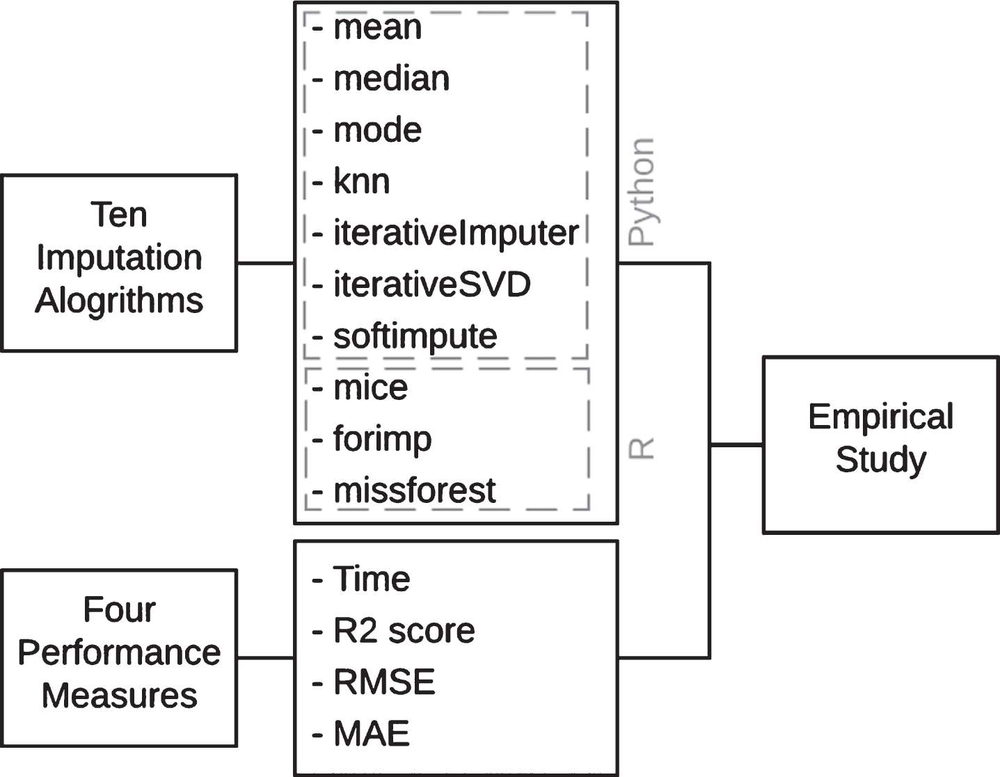
This paper revises the most common imputation algorithms, presents Python and R packages in the comparisons, and evaluates the imputation accuracy from the point of R2 score, RMSE, and MAE (see Fig. 2).
Imputation algorithms and validity measures used in this study.
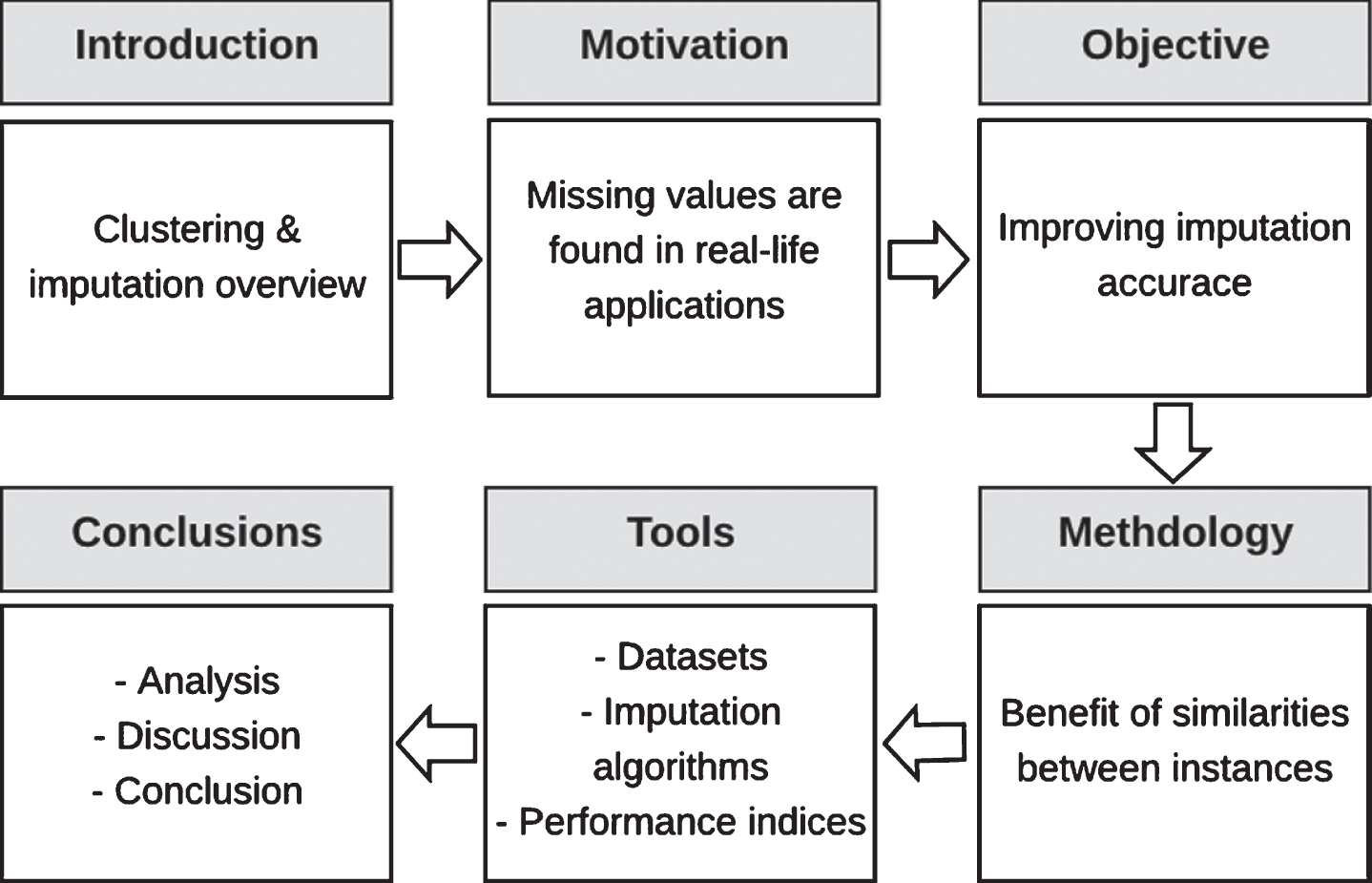
The rest of the paper is organized as follows: Section 2 discusses the literature review, the proposed preprocessing step and the experimental implementation are discussed in Section 3. Summary and conclusion are explained in Section 4. Figure 3 shows the structure of this paper.
Organization of the paper.
This section discusses an overview of the studies related to handling missing values.
Cismondi et al. [36] presented a method for dealing with missing values in intensive care units (ICU) databases to better the modelling performance. By using statistical classifier followed by fuzzy modelling, the authors determined which missing value should be imputed. The authors estimated the performance of the method by developing a test bed. Although their approach improved the classification accuracy, specificity, and sensitivity, their approach may be unsuccessful in filling all missing values. Hapfelmeier et al. [37] considered the problem of the imputation as an optimisation problem. The authors’ proposed framework uses decision tree, KNN, and support vector machine (SVM). Two composite methods (i.e., opt.cv and benchmark.cv) are incorporated in their framework. opt.cv selects the best method from opt.svm, opt.tree, and opt.knn. benchmark.cv selects the best method from iterative KNNs, KNNs, Bayesian principal component analysis mean, and predictive-mean matching. Although their proposed method performed better than other methods, the time used for picking out the best method that gives lowest error was long, in addition to the small size of the data used in the experiments. Batista and Monard [38] compared between some common methods (i.e., KNN, C4.5, and CN2). The authors performed the experiments at different ratio of the missing values. Although the experiments indicate that KNN performed better than C4.5 and CN2, C4.5 is competitive to ten-nearest neighbor in some cases. To assert the analysis significance, the value of the parameter K used should be increased. Aydilek and Arslan [39] combined two methods (support vector regression (SVR) and genetic algorithm (GA)) with fuzzy clustering to fill in missing data. The authors compared their proposed method with SvrGa, FcmGa, and Zeroimpute methods. Although the accuracy of the imputation was better, the size of the complete dataset affects the efficiency of the training phase by SVR, which means that if many variables contain many missing values, many instances will be discarded. Qin et al. [40] proposed a stochastic semi-parametric regression for imputing missing values in semi-parametric data. The authors compared their method with deterministic semi-parametric regression imputation from the point of view of RMSE using simulated and real data experimentally. Although effectiveness and efficiency of their proposed method were better than deterministic semi-parametric imputation, both of RMSE and mean squared error (MSE) are susceptible to the outliers since they give extra weights to large errors [41]. Li et al. [34] took advantage of fuzzy K-means for imputing missing values. Each object belongs to a cluster with a fuzzy membership degree. The authors evaluated the algorithm performance from the RMSE point of view. Depending on the fuzzifier value, K-means may perform better than fuzzy K-means and vice versa, which means that determining the adequate value of the fuzzifier parameter represents an issue. Acuña and Rodriguez [42] compared between four popular approaches, mean imputation, KNN, median imputation, and complete case analysis in supervised classification problems. The comparison was done using 12 datasets. Muñoz and Rueda [43] proposed two imputation approaches based on quantiles. The authors did not benefit from auxiliary information in the first algorithm, whereas they benefited from auxiliary information in the second algorithm. Determining the relationship between the variable of interest and the auxiliary variable is an issue. Batista and Monard [31] applied the measure of Euclidean distance to find the k cases that have the most similarities. Then, it fills in the missing categorical values in the variable of interest using the most frequent value within KNN cases. The missing numerical values are imputed with the unconditional mean. Although the KNN imputation algorithm is simple and its performance is higher than the mean/mode approaches, it is expensive in dataset with large size because it needs to look into as many times as the number of instances which contain missing values to find the nearest neighbours of each instance with missing value(s). Honghai et al. [44] used support vector machine (SVM) to impute missing values. Their work was devoid of any comparison with other imputation algorithms. Furthermore, the size of the training data with no missing values is not enough, which leads that the accuracy of regression will be affected. Pelckmans et al. [45] applied maximum-likelihood approach to get the estimates for the models assumed from their method for the covariates of missing data. The classification rules can be learnt from the data even when the input variables contain missing values, however, the aim of their proposed method is for high classification accuracy rather than high imputation accuracy. Samih [11] proposed a linear regression based algorithm called cumulative linear regression (CLR). His proposed algorithm incorporates the imputed variables into a linear regression equation to filling in the missing values in the subsequent incomplete variable. The author compared his proposed algorithm with eight algorithms namely Mice, ForImp, missForest, Simputation, VIM, IterativeImputer, KNN, and SoftImpute. In some cases, CLR outperforms other algorithms and vice versa. Samih and Hirofumi [46] presented novel technique to improve the accuracy of the prediction by clustering the data using K-means clustering method, and applying the selected prediction algorithm to every cluster. Their proposed approach benefits from the similarities between the cases to improve the prediction accuracy. Samih [47] proposed a new method for imputing missing values by the aid of other features (donors). His proposed method depends on the correlation between the donor and the variable of interest. In addition to the correlation, the number of cases which will be used in the imputation is another factor in the selection. His proposed method is not efficient with the dataset with categorical attributes; it behaves somewhat similar to unconditional mean. The missing values which have not been imputed by the donors will be imputed using another imputation method (i.e., unconditional mean).
Data preprocessing phase
This section gives a more in depth description of the proposed preprocessing phase. In the proposed preprocessing phase, the author takes benefit from the similarity attribute of the data to improve the accuracy of the imputation. Instead of applying the imputation method on the whole data, the proposed preprocessing phase applies the imputation method on each cluster. The proposed method assumes that the dataset is clustered and the number of clusters is known in advance, and the selected imputation algorithm is applied for every cluster.
To give more in depth clarification, an illustrative example is discussed in the next subsection.
Illustrative Example
An artificial data with 130 observations has been created in two clusters. The observations with the missing data are labeled, which means that these observations are already clustered. The positions of the missing values in the figure do not mean that the values are known, they are positioned in order to clarify that these observations belong to this cluster. The missing data in each cluster will be filled by the chosen algorithm with respect to the data in each cluster rather than the whole data. Figure 4 shows the data with missing values and Fig. 5 shows the data after imputation.
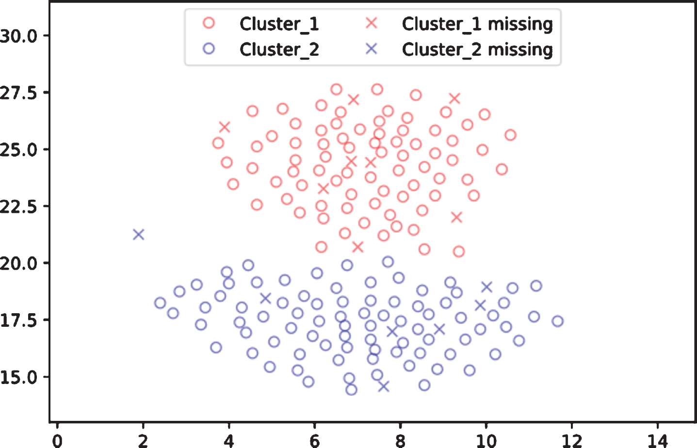
Observations with missing values.

Observations with filled values.
Benchmark datasets
Four datasets that are commonly used in different data bases repository and the literature are used in this comparative study (Table 2). For assessing the performance and generalisation of the methods, the datasets vary on types and numbers of missing values. The author generated the missing values in each dataset under the three types of mechanisms; MAR, MNAR, and MCAR, each type with 10%, 20%, and 30% missingness ratios (MRs)
Datasets specifications
Datasets specifications
The proposed preprocessing technique benefits from the similarity between records in the same cluster which in turn improves the accuracy of the imputation algorithm. Both Python and R provide some imputation algorithms. The comparison is done between ten common imputation algorithms namely mean, median, mode, KNN, IterativeImputer, IterativeSVD, Softimpute, Mice, Forimp, and Missforest. Table 3 gives short descriptions of the prediction algorithms used.
Packages and functions used for experiments
Packages and functions used for experiments
The imputation performance is evaluated using R2, MAE, RMSE and the imputation time in seconds (t).
•RMSE: given by (1), in which y
i
and
•MAE: given by (2)
•R2: given by (3)
•Time of imputation in seconds (t).
The imputation algorithm is considered to be efficient if it imputes in a little time with high accuracy and small error. The experiments were executed using a computer with the following specifications: Intel core i5-2400 (3.10 GHz) processor, 16GB memory, Gnu/Linux Fedora 28 OS, 1TB HDD, and R (version 3.5.2) and Python (version 3.7) programming language.
Table 4, 5, 6, 7 show imputation time, R2 score, RMSE and MAE comparisons of the ten imputation algorithms with and without considering the clustering for flame, jain, pathbased, and aggregation datasets respectively. Figures 6 and 7 show how much improvement is achieved by the proposed algorithm in the aggregation dataset from the point of view of R2 score, and RMSE and MAE respectively. Figures 8 and 9 belong to flame dataset, Figs. 10 and 11 belong to Jain dataset, and Figs. 12 and 13 belong to pathpased dataset.
Imputation time, R2 score, RMSE, and MAE comparison between the ten imputation algorithms with/out considering the clustering (flame dataset )
Imputation time, R2 score, RMSE, and MAE comparison between the ten imputation algorithms with/out considering the clustering (
Imputation time, R2score, RMSE, and MAE comparison between the ten imputation algorithms with/out considering the clustering (
Imputation time, R2score, RMSE, and MAE comparison between the ten imputation algorithms with/out considering the clustering (
Imputation time, R2score, RMSE, and MAE comparison between the ten imputation algorithms with/out considering the clustering (

R2 score Improvement percentage of the proposed algorithm over the compared algorithms (aggregation dataset).
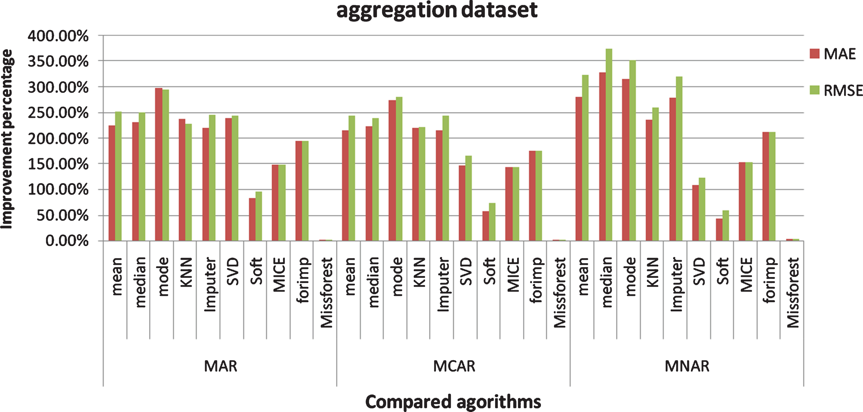
RMSE and MAE Improvement percentage of the proposed algorithm over the compared algorithms (aggregation dataset).
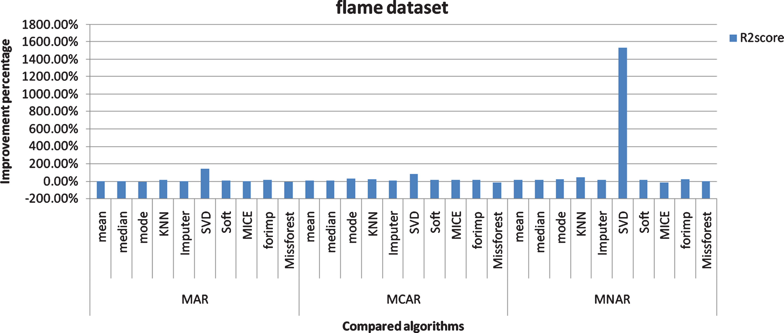
R2 score Improvement percentage of the proposed algorithm over the compared algorithms (flame dataset).

RMSE and MAE Improvement percentage of the proposed algorithm over the compared algorithms (flame dataset).
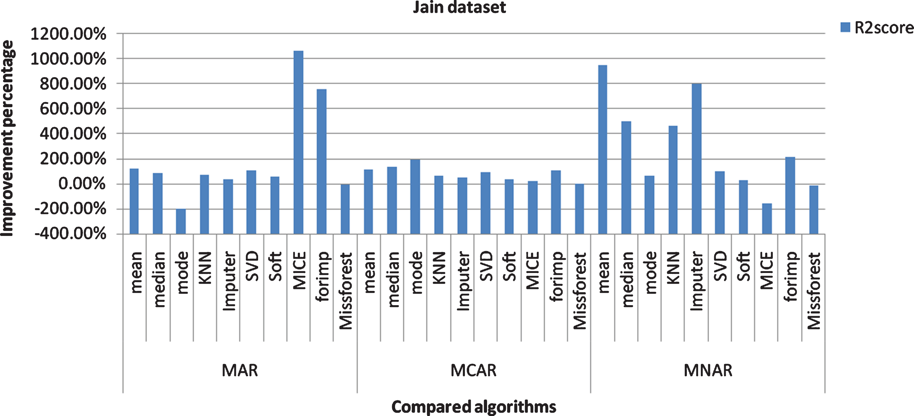
R2 score Improvement percentage of the proposed algorithm over the compared algorithms (Jain dataset).
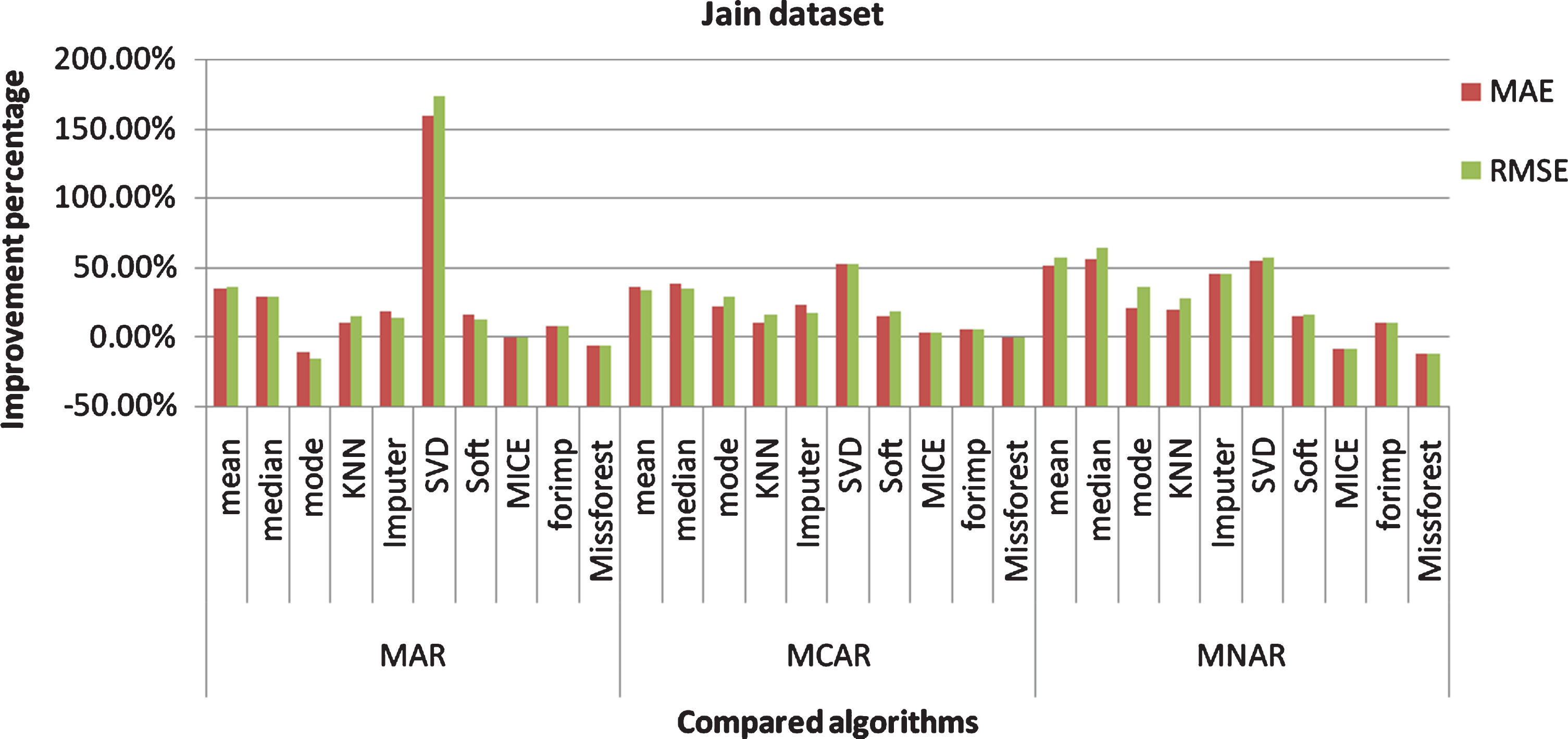
RMSE and MAE Improvement percentage of the proposed algorithm over the compared algorithms (Jain dataset).

R2 score Improvement percentage of the proposed algorithm over the compared algorithms (pathpased dataset).
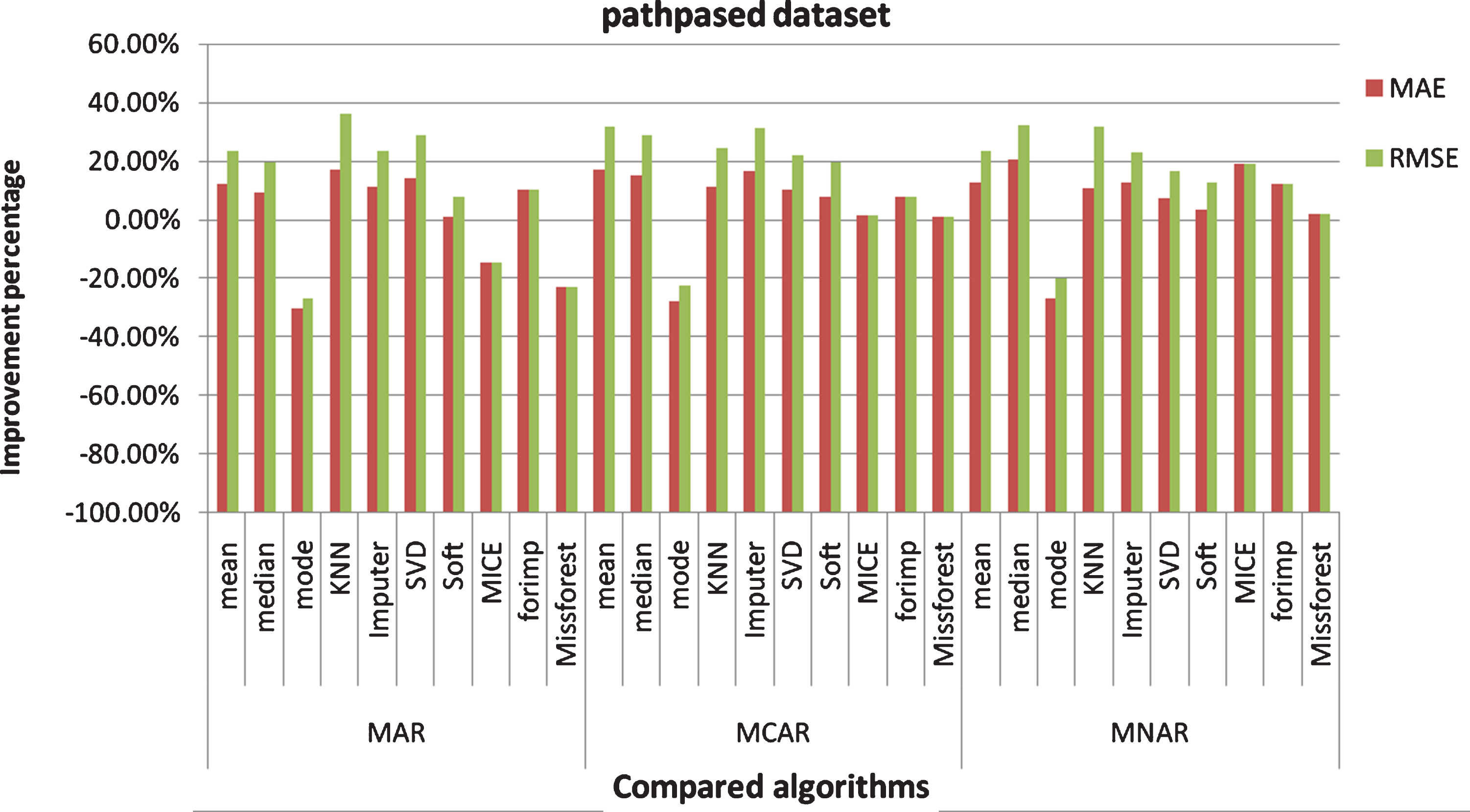
RMSE and MAE Improvement percentage of the proposed algorithm over the compared algorithms (pathpased dataset).
The prominent observations are:
The imputation times for most algorithms when applying them on the whole data are better than the imputation times when applying them on the clustered data.
For flame dataset: The results when applying the imputation algorithms on the clusters are better than applying the imputation algorithms on the whole data, except with the mode algorithm which gives very little better results with the whole data in MAR. The Mice algorithm gives little better results in MNAR. The Missforest gives little better results in MCAR and MAR. In MAR, R2 score of the proposed technique is better than the compared algorithms except for the mode and Missforest algorithms. RMSE of the proposed technique is better than all the compared algorithms except for the mode algorithm. MAE of the proposed technique is better than all the compared algorithms except for the mode and Missforest algorithms. In MCAR, R2 score, RMSE, and MAE of the proposed technique are better than all the compared algorithms except for the Missforest algorithm. In MNAR, R2 score, RMSE, and MAE of the proposed technique are better than all the compared algorithms except for the Mice algorithm.
For jain dataset: The mean algorithm gives better MAE in the three mechanisms. The median algorithm gives better results with the clustered data. The mode algorithm gives better results with the whole data in MAR. The KNN gives better results with the clustered data. The IterativeImputer, IterativeSVD, and Softimpute algorithms give better results with the clustered data. The Mice algorithm gives better results better RMSE and MAE in MAR and MNAR, and gives better R2 score in MAR. The Forimp gives better results with the clustered data in the three mechanisms. The Missforest gives better results with
the whole data in the three mechanisms. In MAR, R2 score, RMSE, and MAE of the proposed technique are better than the compared algorithms except for the mode and Missforest algorithms. RMSE and MAE of the Mice algorithm are better than the proposed technique. In MCAR, R2 score, RMSE, and MAE of the proposed technique are better than all the compared algorithms except for the Missforest algorithm. In MNAR, R2 score, RMSE, and MAE of the proposed technique are better than all the compared algorithms except for the Mice and Missforest algorithms.
For pathbased dataset: The mean, median, KNN, IterativeImputer, IterativeSVD, Softimpute, and Forimp algorithms give better results with the clustered data in the three mechanisms. The mode algorithm gives better results with the whole data in the three mechanisms. The Mice algorithm gives better results with the whole data in MAR, and gives better results with the clustered data in MCAR and MNAR. The Missforest gives better results with the whole data in MAR, and gives better results with the clustered data in MCAR and MNAR. In MAR, R2 score, RMSE, and MAE of the proposed technique are better than the compared algorithms except for the mode, Mice, and Missforest algorithms. In MCAR, R2 score, RMSE, and MAE of the proposed technique are better than all the compared algorithms except for the mode algorithm. In MNAR, R2 score, RMSE, and MAE of the proposed technique are better than all the compared algorithms except for the mode algorithms.
For aggregation dataset: The mean, median, mode, KNN, IterativeImputer, IterativeSVD, Softimpute, Mice, Forimp, and Missforest give better results with the clustered data in the three mechanisms. In MAR, MCAR, and MNAR, R2 score, RMSE, and MAE of the proposed technique are better than the compared algorithms.
Data preprocessing has a considerable impact on the statistical analysis. Handling the missing data is an important stage in the data preprocessing, therefore, it has magnitude significance in data analysis. The problem with existing methods which handle missing values is that they deal with the whole data ignoring the characteristics of the data (e.g., clustered data). The effect of imputing the missing values is investigated in this paper using ten popular imputation algorithms. This paper proposed a preprocessing phase benefiting from the similarity attribute of the data to improve the accuracy of the imputation. The proposed method applies the imputation algorithm in each cluster. The comparative study has been done between ten imputation algorithms under two cases; when applying in each cluster and when applying in the whole data on four datasets with different number of clusters, sizes, and shapes. The empirical study showed better effectiveness from the point of view of imputation time, RMSE, MAE, and R2 score.