An adaptive approach for estimation of transition probability matrix in the interacting multiple model filter

Abstract

The traditional Interacting Multiple Model (IMM) filters usually consider that the Transition Probability Matrix (TPM) is known, however, when the IMM is associated with time-varying or inaccurate transition probabilities the estimation of system states may not be predicted adequately. The main methodological contribution of this paper is an approach based on the IMM filter and retention models to determine the TPM adaptively and automatically with relatively low computational cost and no need for complex operations or storing the measurement history. The proposed method is compared to the traditional IMM filter, IMM with Bayesian Network (BNs) and a state-of-the-art Adaptive TPM-based parallel IMM (ATPM-PIMM) algorithm. The experiments were carried out in an artificial numerical example as well as in two real-world health monitoring applications: the PRONOSTIA platform and the Li-ion batteries data set provided by NASA. The Retention Interacting Multiple Model (R-IMM) results indicate that a better prediction performance can be obtained when the TPM is not properly adjusted or not precisely known.

Keywords

Adaptive systems dynamic systems filtering techniques markov models system state estimation

1 Introduction

Estimating the states of a dynamic system is a fundamental task to ensure certain performance levels in practical industrial applications. However, obtaining some of these measurements may not be possible, which explains the success of Bayesian filtering for real-world problems [1]. In the literature, several estimation problems based on Bayesian filtering assume that one model describes the system dynamics [2 –5], but the system state evolution may implicate the changing of modes, and a single model may not describe the system behavior adequately. In this context, Markov Jump System (MJSs) and Fuzzy Logic System (FLSs) play a substantial role in tasks related to condition-based maintenance, such as fault detection and diagnosis [6, 7], fault prognostics [8, 9], Fault Tolerant Control (FTC) [10 –15], and event-triggered control [16, 17]. A slide mode observer is used in [10] for FTC of mobile manipulator systems described by time-delay Markov Jump System (MJS). In [11], nonlinear simultaneous additive and multiplicative actuator faults are dealt with through MJS and fuzzy logic systems. The fuzzy adaptive control of an electromechanical system with non-affine nonlinear faults is addressed in [12]. [13] presents fuzzy reconfiguration blocks to hide actuator and sensor fault occurrences from the nominal controller, enabling FTC in nonlinear systems. The design of virtual sensors and virtual actuators is addressed in [14], where a robust FTC methodology is employed for linear parameter varying systems. [8] uses a specific type of MJS, namely Interacting Multiple Model (IMM), to predict accelerated rolling bearings’ degradation state, enabling fault prognostics. In [9], a novel incremental Fuzzy Logic System (FLS) is provided for fault prognostics in accelerated rolling bearings. In [6], an IMM approach based on a nonlinear vehicle dynamics observer is employed to detect and isolate faults in driven-by-wire vehicles. [7] uses parallel particle filter estimations combined through IMM to estimate the states of highly nonlinear dynamic processes, allowing fault detection and diagnosis. The IMM filters are methods for adaptive estimation of states that characterize the behavior of dynamic systems with multiple mode operation [8 , 19].

In the IMM filters, the system jumps are modeled by a Markov chain which is reflected by a Transition Probability Matrix (TPM) and it is assumed to be known a priori. However, when this approach is associated with a time-varying or inaccurate transition probabilities it can lead to the misleading state estimation. In order to improve this drawback, different kinds of approaches have been proposed in the literature. In [20], an approximate likelihood function of the TPM is used to determine the TPM according to the maximum likelihood criterion. In [21], the authors present a meta model filter which the transitions are obtained using a Bayesian Network (BN). In [22], a fuzzy decision maker is proposed to choose the TPM from a finite candidate set. In [23], expectation maximization procedure is proposed to estimate the TPM and its performance is shown to be better when compared with the Kullback-Leibler divergence method presented in [24]. Unfortunately, these methods have some disadvantages, as, for example, to be computationally very expensive [21, 23], other ones rely on optimization algorithms [23] or consider that the TPM is obtained from a finite set [22]. Two methodologies to estimate the TPM are presented in [25]; the first technique estimates a continuous Markov chain using missing data and the second uses the full data set to capture the non-Markovian effect of rating momentum. [26] shows four algorithms with minimum mean-square error to recursively estimate the TPM. The first method is used when the TPM is linear in the transition probabilities, but its computational load increases with the data length since the algorithm requires a knowledge of all moments of the Transition Probability Matrix (TPMs) prior probability density function. The second method considers that the third central moments are zero to create a second-order approximation for the TPM, which can yield numerical problems in estimating the TPM. The third method assumes a Dirichlet distribution for the prior probabilities of a finite mixture used to estimate the TPM. At the same time, the fourth approach straightforwardly integrates over a finite grid of the TPM posterior probability density function, increasing its computational burden. [27] provides an algorithm to adapt the TPM in maneuvering target tracking tasks; the computation relies on the speed of the target and the radius of the turn which restricts the application to systems with such sensors. Moreover, TPM uncertainty is considered in [28], where a polytopic set with multiple Transition Probability Matrix (TPMs) is used in the design of robust model predictive control. Less conservative conditions were obtained for state-feedback control, increasing the maximal feasible region for the systems’ states while ensuring mean square stability and satisfaction of hard constraints on system inputs and states. Time-varying Transition Probability Matrix (TPMs) are considered in [29] with values estimated at each time step by solving a linear programming optimization problem. The method imposes that the observed multivariate time series needs to be non-negative and that its normalized values are realizations of the stationary distribution of the modeled Markov process. For the parallel IMM algorithm, [30] proposed a technique to correct the TPM in a recursive way using the gradient of the model probability. This correction is improved by doubling the number of filters to bring in the information of the current model upon model jumps. However, in order to identify these jumps, a constant threshold is introduced; this threshold must be defined according to the problem.

To overcome the problem of unknown Transition Probability Matrix (TPMs) in nonlinear time-varying systems and to reduce the conservativeness regarding previous assumptions and required pre-defined thresholds, this paper proposes an approach based on the concept of retention model presented by [31] which tests hypothesis between constancy and free variation of transition probabilities applied to a panel study of voting intentions prior to the 1940 election in the US. The relatively low cost is very attractive to the estimation of the transition probabilities in the context of the IMM filter for real-world online applications. This work differs from [31] by introducing the adaptive feature and by ensuring that less parameters need to be estimated. The main contributions of this paper are summarized as follows:

the unknown transition probability is determined adaptively and automatically at each instant k;

a method with relatively low computational cost is presented which has no need for complex operations or storing the measurement history;

a new approach is proposed based on IMM and the retention model concept to allow the TPM be time-varying.

The remainder of this paper is organized as follows. Section 2 presents the problem formulation that will be addressed in this paper and a brief overview of the IMM theory. Section 3 provides details on the proposed approach that applies the retention model concept to estimate the TPM used in IMM recursively. Section 4 shows three experiments to test the proposed approach against the traditional IMM, a method that uses Bayesian Network (BNs) with IMM [21] and a state-of-the-art Adaptive TPM-based parallel IMM (ATPM-PIMM) proposed in [30]. The first experiment is a toy example with two different switching transition models where the influence of inaccurate Transition Probability Matrix (TPMs) is studied, showing the robustness of the proposed approach. The second experiment consists of a real-world experiment of monitoring real rolling bearings’ health in the PRONOSTIA platform [32]. The third experiment concerns the degradation of four Li-ion batteries provided by a testbed in the NASA Ames Prognostics Center of Excellence (PCoE) [33]. Finally, Section 5 draws the final remarks.

2 Problem formulation

Consider the following discrete-time MJS: $x_{k} = f (x_{k - 1}, θ_{k}, ω_{k})$ (1) $y_{k} = h (x_{k}, θ_{k}, η_{k})$ (2)

where $k \in ℕ$ is the time instant, $x_{k} \in ℝ^{n}$ is the unknown state vector, $y_{k} \in ℝ^{m}$ is the measurement, ω_k and η_k are the process and measurement noises, respectively, and θ_k is a finite state Markov chain with a TPM R. The state transition function, possibly nonlinear, is given by f and h is the measurement equation, possibly nonlinear as well.

According to [18], the IMM output uses the law of total probability defined by: $p (x_{k} | y_{k}) = \sum_{j}^{N} p (x_{k} | θ_{k} = j, y_{k}) p (θ_{k} = j | y_{k}) ThickSpace .$ (3) The posteriori probability density p (x_k|y_k) given in (3) is reached by combining the probability density functions of models which are conditionally dependent on measurement y_k.

Unfortunately, the IMM filter may not obtain good estimates in cases when the available TPM is not accurate. For instance, consider a state space system with inaccurate transition probability in which the state vector is estimated by model 1 up to instant k = 150 and by model 2 after that. Fig. 1 depicts a two model example with true and predicted states by the IMM algorithm. The figure also shows the model probabilities. In this case, model 1 is expected to have higher probability values (y-axis) than model 2 before k = 150 and, after this instant, model 2 becomes dominant. However, as the TPM is not accurate, Fig. 1 depicts that the dominant model becomes model 2 before the expected instant (k = 150). After k = 150 the model 1 is dominant, and that is the reason IMM does not predict the true system states.

Fig. 1

State estimation and model probabilities obtained by the IMM method with wrong TPM matrix.

This uncertainty can be explained by observing the TPM used to estimate these states: $\begin{matrix} TPM = [\begin{matrix} 0.4 & 0.6 \\ 0.6 & 0.4 \end{matrix}] \end{matrix}$

In this case, the matrix shows that the probability of remaining in the same state is less than changing to a new state, which does not correspond to the true matrix, as can be seen: $\begin{matrix} TPM = [\begin{matrix} 0.99 & 0.1 \\ 0 & 1 \end{matrix}] \end{matrix}$

To overcome the aforementioned problem, a new approach is proposed based on IMM and the retention model concept [31]. This new approach is called Retention Interacting Multiple Model (R-IMM) and it will include Particle Filters since they are very suitable to deal with nonlinear and non-Gaussian scenarios [34 –37].

2.1 IMM method

The traditional IMM proposed by [38] has the following steps:

Model mixing and

State interacting that represent the interaction of model estimates at the beginning of each estimation cycle;

Filtering stage, which executes each model, in parallel;

Combination stage that estimates the current state based on the output of all models.

The model mixing and state interacting depend on the predicted model probability from the previous estimates and the TPM R. The model transition is defined by a Markov process and the switch probability p (θ_k = i|θ_k-1 = j) = R_ij denotes the transition probability from model i to model j. However, this matrix is assumed to be known a priori. The Chapman-Kolmogorov equation for the model mixing is: $p (θ_{k} = i | y_{k - 1}) = \sum_{j} R_{ij} p (θ_{k - 1} = j | y_{k - 1}) ThickSpace .$ (4) At the filtering stage, a filter is performed for each of the N models and this step follows the evolution system (1). The update of each filter is done following (2) and based on the predicted states. Finally, the state of the system is estimated by the weighted sum of the probabilities of all filters and their respective outputs.

3 Proposed retention IMM

This paper uses the concept of retention model proposed in [31] which tests hypothesis between constancy and free variation of transition probabilities. This approach can specify the way in which the transition matrices vary in time. Here, we apply the retention model in the context of the IMM filter, with the difference that the TPM is unknown a priori and it is calculated along the IMM procedure. This methodology also ensures that less parameters need to be estimated each time instant. Let {θ_k, k = 0, 1, …, T} be an N state Markov chain and its transition probabilities are defined by: $\begin{matrix} R_{ijk} = p (θ_{k} = j | θ_{k - 1} = i), ThickSpace i, j = 1, \dots, N ThickSpace, \\ 0 \leq R_{ijk} \leq 1, ThickSpace \sum_{j = 1}^{N} R_{ijk} = 1, ThickSpace i, j = 1, \dots, N ThickSpace . \end{matrix}$ (5) where R is the matrix of transition probabilities from instants k - 1 to k.

According to [31], a Markov chain can be the combination of two processes: the first process determines when a transition between two distinct states will occur; and the second one determines the outcome of the move. Following this approach with two matrices D_k and M_k, the decomposition of the transition matrix is defined as follows: $R_{k} = D_{k} + (I - D_{k}) M_{k} ThickSpace,$ (6) where D_k is a matrix containing the diagonal entries of R_k (d_ijk = 0 for i ≠ j) and M_k is defined as m_ijk = p (θ_k = i|θ_k-1 = j, θ_k ≠ j). Therefore, m_ijk = 0 for all i = j and m_ijk = R_ijk/(1 - R_ijk). Provided that each row of m_k sums to one: $d_{ik} = n_{ijk} / n_{i . k}$ (7) $m_{ijk} = n_{ijk} / (n_{i . k} - n_{iik}), i \neq j$ (8) where n_ijk is the number of transitions from state i to state j at instant k and n_i.k is the total of transition to state i.

In [31], the matrices M and D are calculated from all available transitions from instant 1 up to T, thus if M_k = M, D_k is still given by (7), but m_ij = n_ij/(n_i - n_ii) , ThickSpace i ≠ j, where n_ij and n_i are calculated from all available transitions. Lastly, when D_k = D, and M_k changes, M_k is (8) and d_i = n_ii/n_i.

As the IMM method is calculated recursively and the transition matrix is considered not known, this work proposes a few modifications so that R is also calculated recursively. Consider that matrices D₀ and M₀, at instant k = 0, are provided by the user, the active model (θ_k) at instant k is the one with the highest model probability calculated by IMM and D_k-1 and M_k-1 are matrices calculated at instant k - 1. Thus, if M_k = M_k-1, D_k is still given by (7), and $m_{ij k - 1} = n_{ijk - 1} / (n_{ik - 1} - n_{iik - 1}), i \neq j$ (9) where n_ijk-1 and n_ik-1 are calculated from the number of transitions at instant k - 1. Lastly, when D_k = D_k-1, and M_k changes, M_k is (8) and $d_{ik - 1} = n_{iik - 1} / n_{ik - 1}$ (10) Similarly to [31], some hypotheses for the transition probabilities are considered: $\begin{matrix} H_{0} : & R_{k} = R_{k - 1} = D_{k - 1} + (I - D_{k - 1}) M_{k - 1} \\ H_{1} : & R_{k} = D_{k} + (I - D_{k}) M_{k - 1} \\ H_{2} : & R_{k} = D_{k - 1} + (I - D_{k - 1}) M_{k} \\ H_{3} : & R_{k} = D_{k} + (I - D_{k}) M_{k} \end{matrix}$ (11) The degrees of freedom consider the number of independent parameters to be estimated under each hypothesis. There is one transition matrix calculated at instant k, so each one containing m (m - 1) independent parameters to be estimated. The transition matrices for each hypothesis are defined by $\begin{matrix} R_{ijk}^{0} = & d_{ijk - 1} + (1 - d_{iik - 1}) m_{ijk - 1} \\ R_{ijk}^{1} = & d_{ijk} + (1 - d_{iik}) m_{ijk - 1} \\ R_{ijk}^{2} = & d_{ijk - 1} + (1 - d_{iik - 1}) m_{ijk} \\ R_{ijk}^{3} = & d_{ijk} + (1 - d_{iik}) m_{ijk} \end{matrix}$ (12) Following [31], χ ² tests are used to determine the hypotheses $χ_{0, 1}^{2}$ and $χ_{1, 2}^{2}$ and $χ_{2, 3}^{2}$ , which are: $\begin{matrix} χ_{0, 1}^{2} = & \sum_{k} \sum_{i} n_{i . k} \sum_{j} (R_{ijk}^{1} - R_{ijk}^{0})^{2} / R_{ijk}^{0} \\ χ_{1, 2}^{2} = & \sum_{k} \sum_{i} n_{i . k} \sum_{j} (R_{ijk}^{2} - R_{ijk}^{1})^{2} / R_{ijk}^{1} \\ χ_{2, 3}^{2} = & \sum_{k} \sum_{i} n_{i . k} \sum_{j} (R_{ijk}^{3} - R_{ijk}^{2})^{2} / R_{ijk}^{2} \end{matrix}$ (13) To avoid numerical problems during the construction of matrices, when the number of transitions n_ij from state i to state j is equal to 0, it is added a constant c₁ to n_ij or c₂, otherwise. At the end of the process of creating the TPM at time k, the new matrix calculated by the proposed method will replace R_i,j in (4). The retention model algorithm that updates the TPM recursively can be summarized as follows:

Find matching models μ_k-1 and μ_k

Increment n_{μ_k-1,μ_k,k}

Compute D_k using (7) and D_k-1 using (10)

Compute M_k using (8) and M_k-1 using (9)

Run the χ ² tests in (13) to update the TPM:

If $χ_{0, 1}^{2} \leq η$ : choose hypothesis H₀

Else if $χ_{1, 2}^{2} \leq η$ : choose hypothesis H₁

Else if $χ_{2, 3}^{2} \leq η$ : choose hypothesis H₂

Else: choose hypothesis H₃

where η = χ ² (0.95, ν) is the chi-square inverse cumulative distribution function at 95% confidence level and ν degrees of freedom, which it is defined by the number of independent TPM parameters.

4 A numerical experiment and two monitoring applications

In this section, we consider a numerical experiment and two real-world monitoring applications to compare the performance of the proposed algorithm (R-IMM) with the following methods: the IMM algorithm, the IMM with BN (BN-IMM) [21], and the ATPM-PIMM algorithm [30]. According to [30], the threshold for ATPM-PIMM can be set to 0.8 so the algorithm can achieve a good performance on both noise smoothing and response speed to the model jump. The Root Mean Squared Error (RMSE) and Mean Absolute Percentage Error (MAPE) are employed to measure the performance of the filters. The simulations use thirty independent experiments, 50 particles and the systematic resampling method [34].

4.1 Illustrative experiment

Consider the state space models: $x_{k} = {\begin{matrix} α_{1} x_{k - 1} + α_{2} + ω_{k}^{1}, & if k < \frac{T}{2} \\ α_{3} x_{k - 1}^{α_{4}} + x_{k - 1} + ω_{k}^{2}, & otherwise \end{matrix}$ (14) $y_{k} = - 4 x_{k}^{(1 / 2)} + η_{k},$ (15)

where T is the maximum simulation time, x_k is the system state, y_k is the measurement, $w_{k}^{j} \sim N (0, σ_{ω}^{2})$ , for j = 1, 2 with σ_ω = 0.002 and $η_{k} \sim N (0, σ_{η}^{2})$ with σ_η = 0.04. The parameters α_i, for i = 1, 2, 3, 4 are [0.986 0.31 0.001 0.835], respectively. The initial state is drawn considering x₀ ∼ N (20, σ_ω). As explained before, to avoid numerical issues, the constants c₁ and c₂ are selected as 1 and 1000, respectively.

The TPM R is usually assumed to be known a priori, but, in real-world problems, it may be unknown. To overcome this problem, the transition probability is calculated recursively by R-IMM. Some scenarios are presented in this paper to illustrate that the proposed R-IMM is more robust than the IMM method especially in the situations in which there is uncertainty about matrix R. In this case, the matrices R_{s
₁}, R_{s
₂}, R_{s
₃} and R_{s
₄} will be used into the traditional IMM. To study the influence of inaccurate TPM, some scenarios are defined: $\begin{matrix} R_{s_{1}} = [\begin{matrix} 0.7 & 0.3 \\ 0.3 & 0.7 \end{matrix}] \\ R_{s_{2}} = [\begin{matrix} 0.6 & 0.4 \\ 0.4 & 0.6 \end{matrix}] \\ R_{s_{3}} = [\begin{matrix} 0.4 & 0.6 \\ 0.6 & 0.4 \end{matrix}] . \end{matrix}$ Additionally, assume that the true TPM, say R_{s
₄}, is the transition rate R_ij = c_ij/∑_jc_ij, where c_ij represents the number of transitions from state i to state j in the training data. These matrices, R_{s
₄} and the initial probability transition matrix for R-IMM (R_ij0), are defined as

$\begin{matrix} R_{s_{4}} = [\begin{matrix} 0.9933 & 0.0067 \\ 0 & 1.0000 \end{matrix}] \\ R_{ij 0} = [\begin{matrix} 0 & 1 \\ 1 & 0 \end{matrix}] \end{matrix}$

Table 1 presents the state estimation results for the proposed scenarios considering different methods. The traditional IMM results are worse as the uncertainty increases in the TPM. The BN-IMM results remain stable because they do not depend on the matrix R; however, it calculates the matrix recursively based on all previous measurements, which is computationally costly. As this method depends on the previous data, it takes time to recognize the change of the active model since there is still no information about the model 2. The proposed method R-IMM does not use all previous measurements and yet it can correctly estimate the transition probability and the states. This fact suggests that the R-IMM with unknown matrix R is able to estimate the states close to true value, as can be noticed from the values highlighted in bold in Table 1.

Table 1

RMSE and MAPE metrics’ mean and standard deviation for 30 independent experiments of state estimation in the illustrative experiment 4.1, with best values in bold

Scenario	Metric	Method
		IMM	BN-IMM	R-IMM	ATPM-PIMM
1	RMSE	0.1417 ± 0.0058	0.2339 ± 0.1131	0.0530 ± 0.0381	0.1376 ± 0.0016
	MAPE	0.5535 ± 0.0219	0.6315 ± 0.3246	0.1906 ± 0.1610	0.5109 ± 0.0077
2	RMSE	0.1681 ± 0.0058	0.2091 ± 0.0850	0.0714 ± 0.0430	0.1576 ± 0.0019
	MAPE	0.6487 ± 0.0220	0.6169 ± 0.2646	0.2667 ± 0.1837	0.5842 ± 0.0095
3	RMSE	0.1964 ± 0.0061	0.2084 ± 0.0211	0.1212 ± 0.0075	0.1776 ± 0.0017
	MAPE	0.7549 ± 0.0223	0.8580 ± 0.0727	0.4848 ± 0.0283	0.6423 ± 0.0086
4	RMSE	0.0223 ± 0.0066	0.2609 ± 0.1568	0.0351 ± 0.0126	0.0249 ± 0.0020
	MAPE	0.0725 ± 0.0216	0.6234 ± 0.4296	0.1126 ± 0.0402	0.0816 ± 0.0093

It is also worth noting that scenario 4 provides the true TPM for the IMM, so no uncertainty related to the transition matrix is provided to the traditional method. Yet, the proposed R-IMM can correctly estimate the states, even if its initial TPM is completely different, as can be seen by R_ij0.

For illustration purposes, Fig. 2 depicts the state predicted by the IMM, BN-IMM and the proposed R-IMM for scenario 3, which is the scenario with greater uncertainty in the TPM defined a priori.

Fig. 2

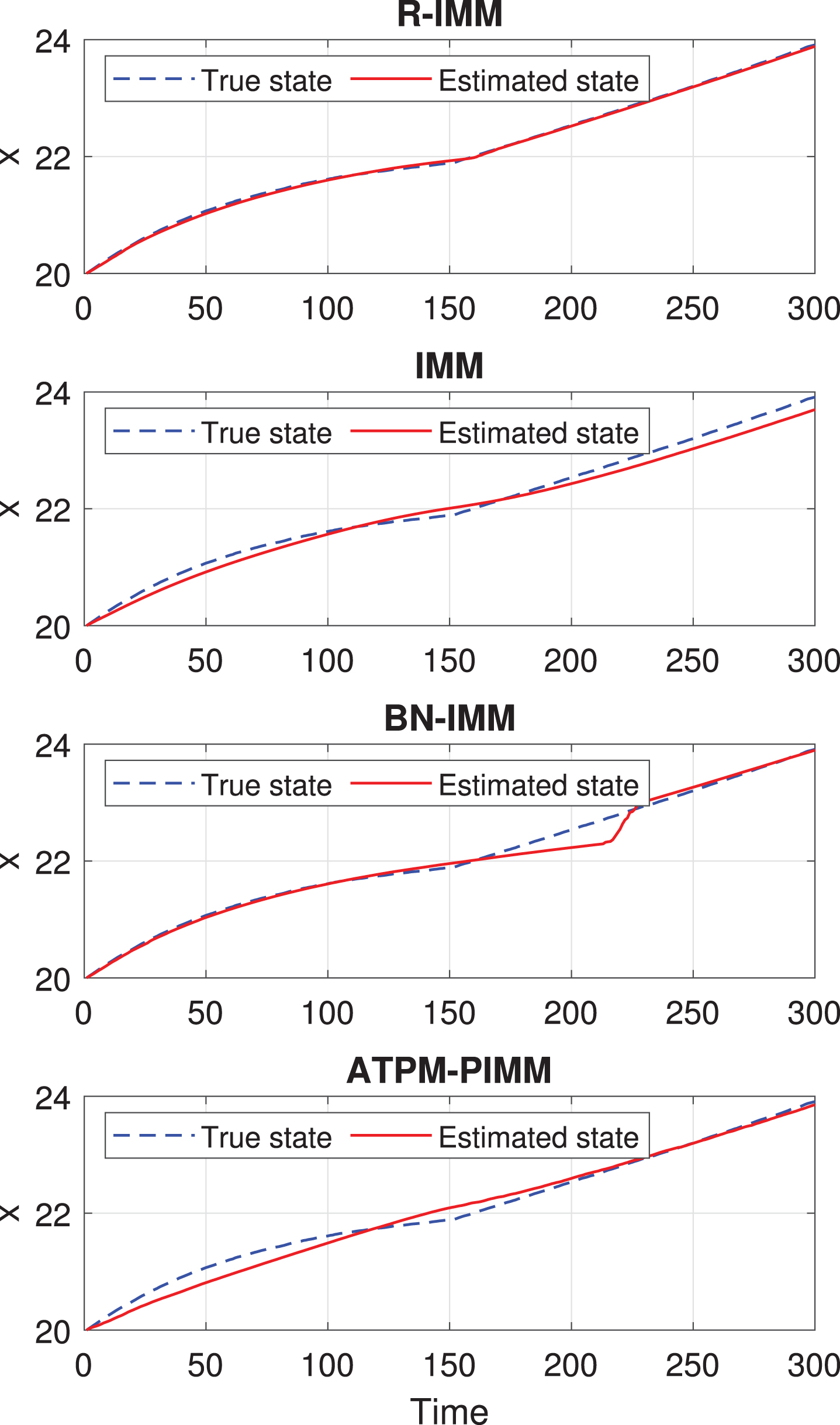
State estimation of IMM, BN-IMM, ATPM-PIMM, and R-IMM, respectively, for scenario 1. Experiment 4.1.

4.2 Health monitoring experiment - PRONOSTIA

The database PRONOSTIA [32] is focused on the estimation of the remaining life of bearings under operating conditions. The extraction and selection of bearings features is based on vibration sensor and here it is used the same procedure and the health indicator proposed in [39]. Three different loads data were considered in the dataset. According to [32], theoretical estimated life durations (L10, BPFI, BPFE, etc.) do not provide the same estimations than those reached by the experimental observations. In this case, two models are extracted for each operating condition using a fuzzy inference system, in the same way as it was proposed in [8]. The proposed R-IMM procedures applied to PRONOSTIA database is divided into two phases. In the first, the models are extracted in the offline training step but, in the second phase, the R-IMM only uses the fuzzy models as system models in the filtering step. In the training, Takagi-Sugeno fuzzy models are used for which the input variables x_k-1 are assigned the N membership functions. The fuzzy IF-THEN rules generated are presented below:

Rule 1: IF x_k-1 is A¹ THEN

x_{k}^{1} = p^{1} x_{k - 1} + q^{1}

⋯

Rule N: IF x_k-1 is A^N THEN

x_{k}^{N} = p^{N} x_{k - 1} + q^{N}

where x_k-1 is the predicted state at instant k - 1, A ^j, j = 1, …, N is the fuzzy set, $x_{k}^{j}$ is the estimated state according to the jth fuzzy rule, p ^j and q ^j are fuzzy model parameters which are determined by learning process. Gaussian combination membership functions are used with four parameters and they also are determined by learning process. After the training step, the models $x_{k}^{j} = p^{j} x_{k - 1} + q^{j}$ will be incorporated into the R-IMM process as the two system models: $\begin{matrix} x_{k}^{1} = p^{1} x_{k - 1}^{1} + q^{1} + w_{k}^{1} \\ x_{k}^{2} = p^{2} x_{k - 1}^{2} + q^{2} + w_{k}^{2} \end{matrix}$ (16) The parameters (p,q) of the two models for each operating condition are given in Table 2.

Table 2

Parameters of the fuzzy systems for Experiment 4.2

Operating Condition	Model	p	q
1	Model 1	0.9956	0.0628
	Model 2	0.9989	0.0395
2	Model 1	0.9911	0.0862
	Model 2	0.9967	0.0712
3	Model 1	0.9902	0.0900
	Model 2	0.9975	0.0528

The filter simulation parameters are σ_ω = 0.0215 and σ_η = 0.2, for process and measurements noises, respectively. The inaccurate TPM R is given as: $R = [\begin{matrix} 0.40 & 0.60 \\ 0.60 & 0.40 \end{matrix}] .$ (17)

The initial probability transition matrix for all methods is given as an identity matrix. Table 3 summarizes the analysis results of the three operating conditions, which helps to understand the merits of the proposed approach in terms of RMSE and MAPE metrics. For each bearing, 30 independent experiments were done to allow statistical comparison between the methods; the results are depicted as the average value with the standard deviation for each group of 30 runs and the best results are highlighted in bold. For the PRONOSTIA database, the conventional IMM has great variability of performance and they are significantly worse than the R-IMM in some cases. This diversity of results also shows that IMM is very sensitive to TPM uncertainty. For the sake of simplicity, all operating conditions are dealt with the same parameters. It is important to note that the results in Table 3 shows a consistent improvement of the accuracy when using the proposed approach. The mean value of both metrics is also compared two by two in Table 4 using the two-sample Student’s t-test. All p-values at a 99% confidence level are significantly lower than 0.01, showing strong evidence to reject the null hypothesis. This indicates that the proposed method’s performance is statistically different than the other approaches’ while it is consistently better in terms of RMSE and MAPE.

Table 3

RMSE and MAPE metrics’ mean and standard deviation for 30 independent experiments of degradation state estimation in the PRONOSTIA dataset, with best values in bold –Experiment 4.2

Bear.	RMSE				MAPE
	IMM	BN-IMM	R-IMM	ATPM-PIMM	IMM	BN-IMM	R-IMM	ATPM-PIMM
1.3	0.24 ± 0.00	2.15 ± 0.02	0.12 ± 0.00	1.37 ± 0.02	1.89 ± 0.03	6.11 ± 0.08	0.94 ± 0.09	7.25 ± 0.01
1.4	0.31 ± 0.00	1.52 ± 0.03	0.13 ± 0.00	1.74 ± 0.01	2.66 ± 0.04	4.29 ± 0.08	1.22 ± 0.07	11.64 ± 0.10
1.5	0.21 ± 0.00	1.10 ± 0.02	0.15 ± 0.01	1.29 ± 0.01	1.79 ± 0.02	3.90 ± 0.08	1.18 ± 0.10	7.16 ± 0.08
1.6	0.21 ± 0.00	1.61 ± 0.02	0.12 ± 0.00	1.33 ± 0.01	1.70 ± 0.02	5.28 ± 0.09	0.93 ± 0.03	6.85 ± 0.08
1.7	0.25 ± 0.00	1.49 ± 0.03	0.12 ± 0.00	1.39 ± 0.01	2.03 ± 0.02	4.87 ± 0.08	0.96 ± 0.07	7.30 ± 0.09
2.3	0.24 ± 0.00	4.08 ± 0.03	0.13 ± 0.00	1.47 ± 0.01	1.75 ± 0.01	17.34 ± 0.14	1.02 ± 0.03	8.47 ± 0.09
2.4	0.31 ± 0.00	0.69 ± 0.02	0.21 ± 0.00	2.35 ± 0.01	3.74 ± 0.06	4.45 ± 0.12	2.15 ± 0.09	23.22 ± 0.29
2.5	0.31 ± 0.00	3.64 ± 0.04	0.15 ± 0.00	1.53 ± 0.03	1.82 ± 0.01	14.28 ± 0.2	1.09 ± 0.02	6.86 ± 0.15
2.6	0.48 ± 0.00	0.25 ± 0.01	0.18 ± 0.00	2.39 ± 0.01	6.23 ± 0.06	2.48 ± 0.09	2.18 ± 0.08	25.94 ± 0.22
2.7	0.52 ± 0.00	0.14 ± 0.00	0.14 ± 0.00	4.27 ± 0.04	9.92 ± 0.15	3.46 ± 0.15	3.44 ± 0.15	73.56 ± 0.88
3.3	0.37 ± 0.00	0.23 ± 0.01	0.20 ± 0.01	3.05 ± 0.03	6.18 ± 0.09	3.09 ± 0.13	3.40 ± 0.16	43.01 ± 0.48

Table 4

p-values for the two-sample Student’s t-test comparing the average RMSE two by two between the proposed R-IMM and IMM, BN-IMM, and ATPM-PIMM at a 99% confidence level. Experiment 4.2

Bearing	Method
	IMM	BN-IMM	ATPM-PIMM
1.3	1.65 · 10^- 54	2.54 · 10^- 94	1.15 · 10^- 97
1.4	4.79 · 10^- 70	7.66 · 10^- 89	1.48 · 10^- 111
1.5	1.71 · 10^- 37	1.26 · 10^- 85	1.17 · 10^- 99
1.6	2.67 · 10^- 55	5.98 · 10^- 99	4.57 · 10^- 103
1.7	6.24 · 10^- 74	1.61 · 10^- 94	1.10 · 10^- 104
2.3	2.89 · 10^- 63	3.22 · 10^- 102	1.65 · 10^- 102
2.4	6.48 · 10^- 52	1.98 · 10^- 67	2.60 · 10^- 109
2.5	9.85 · 10^- 78	2.14 · 10^- 97	6.49 · 10^- 88
2.6	2.71 · 10^- 78	7.47 · 10^- 35	2.06 · 10^- 112
2.7	9.96 · 10^- 78	3.92 · 10^- 01	4.01 · 10^- 107
3.3	6.63 · 10^- 55	7.18 · 10^- 10	1.43 · 10^- 105

The proposed R-IMM presented better performance for all cases without knowing the true TPM and without storing all the measurements. The BN-IMM method did not achieve good results especially in cases in which there were transitions of the states. For example, there was no transition in bearing 2.7, thus the BN-IMM results were the same as the R-IMM.

In the same way as in the previous numerical example, assume that the true TPM, called R, is the transition rate R_ij = c_ij/∑_jc_ij and it is obtained by the training data. This matrix is defined as $R = [\begin{matrix} 0.99 & 0.01 \\ 0 & 1.0000 \end{matrix}] .$ (18)

Table 5 shows the comparative results between the IMM with the true TPM (18) and the R-IMM with a different TPM. The results of 30 independent experiments are shown in terms of average and standard deviation for each metric. The p-value of a two-sample Student’s t-test for the mean is also shown to provide a statistical comparison between the results at a 99% confidence levels, where the * symbol in the bearing column denotes p-values greater than 0.01, which indicate a failure in rejecting the null hypothesis. As can be seen in the Table 5, the performance of the proposed method is practically equivalent to the IMM that uses the true transition matrix, which shows the ability of R-IMM to replace the need for prior knowledge of TPM.

Table 5

Comparative RMSE and MAPE metrics between the IMM using the true TPM and R-IMM from 30 independent experiments with the two-sample Student’s t-test for the mean. The best values are in bold and * denotes results with no statistical difference –Experiment 4.2

Bearing	RMSE			MAPE
	IMM	R-IMM	p-value	IMM	R-IMM	p-value
1.3	0.1095 ± 0.0036	0.1205 ± 0.0102	6.1670 · 10^- 7	0.8437 ± 0.0275	0.9496 ± 0.0974	3.7324 · 10^- 7
*1.4	0.1341 ± 0.0060	0.1332 ± 0.0059	5.5911 · 10^- 1	1.2158 ± 0.0548	1.2043 ± 0.0493	3.9848 · 10^- 1
1.5	0.1310 ± 0.0041	0.1545 ± 0.0112	1.6710 · 10^- 15	0.9617 ± 0.0364	1.1948 ± 0.1034	8.0262 · 10^- 17
1.6	0.1227 ± 0.0044	0.1270 ± 0.0059	1.9496 · 10^- 3	0.9014 ± 0.0338	0.9398 ± 0.0622	4.2631 · 10^- 3
*1.7	0.1218 ± 0.0047	0.1256 ± 0.0074	2.0412 · 10^- 2	0.9391 ± 0.0316	0.9699 ± 0.0671	2.6982 · 10^- 2
*2.3	0.1390 ± 0.0050	0.1396 ± 0.0058	6.6744 · 10^- 1	1.0085 ± 0.0309	1.0225 ± 0.0377	1.2034 · 10^- 1
*2.4	0.2182 ± 0.0124	0.2093 ± 0.0111	5.1748 · 10^- 3	2.1662 ± 0.0951	2.1193 ± 0.0735	3.6775 · 10^- 2
*2.5	0.1571 ± 0.0040	0.1558 ± 0.0054	2.8053 · 10^- 1	1.0830 ± 0.0254	1.0781 ± 0.0406	5.7085 · 10^- 1
*2.6	0.2046 ± 0.0119	0.1888 ± 0.0086	2.0831 · 10^- 7	2.2348 ± 0.1067	2.1827 ± 0.0793	3.5913 · 10^- 2
*2.7	0.1477 ± 0.0072	0.1481 ± 0.0094	8.6306 · 10^- 1	3.4254 ± 0.1552	3.4492 ± 0.2042	6.1350 · 10^- 1
3.3	0.1358 ± 0.0063	0.2074 ± 0.0106	1.8119 · 10^- 38	2.3660 ± 0.0954	3.4008 ± 0.1645	7.2502 · 10^- 37

The main difference between the results in Tables 3 and 5 is that, in the first, the same TPM (given in (17)) is used for all filters to illustrate their sensitivity to uncertain estimations of the real TPM. The latter shows the robustness of the proposed method; the results are similar to the IMM with the real TPM, even when the initial TPM in R-IMM is wrong.

For illustration purposes, Fig. 3 depicts the state estimation of one simulation of bearing 3-3 obtained by the IMM filter with accurate TPM and the proposed R-IMM filter.

Fig. 3

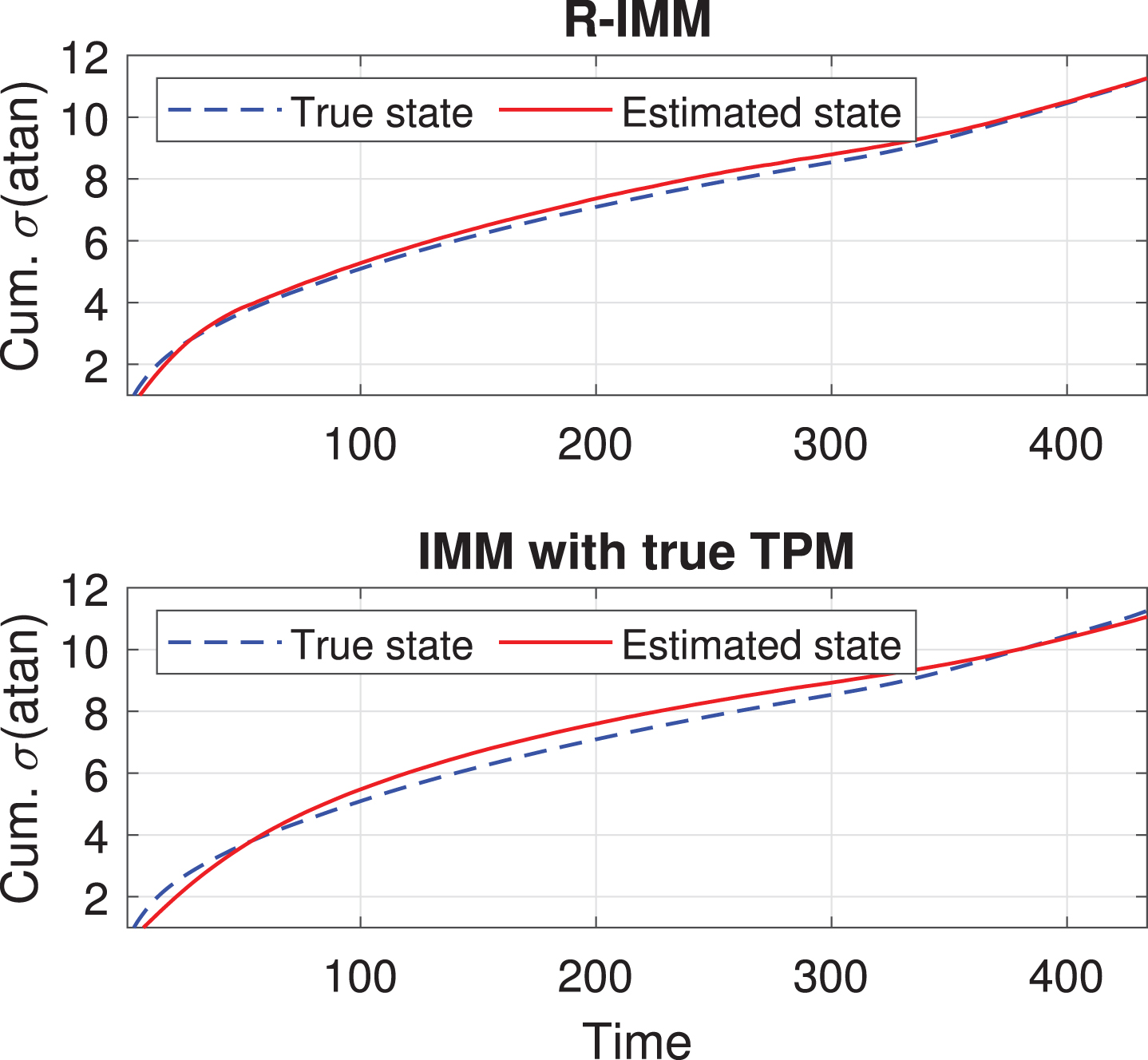
State estimation of IMM and R-IMM, respectively, for bearing 3-3. Experiment 4.2.

Considering the case study, when comparing filter estimates, the proposed R-IMM approach can estimate the states in all testing sets. It can also be observed that the models extracted by the fuzzy inference system were able to model adequately the dynamics of the state derived from the data.

4.3 Health monitoring experiment –Lithium-ion batteries

The case study reported in this section concerns the degradation of Li-ion batteries. This type of battery is found in industry and commercially, e.g., in electric vehicles, microgrids and electronic devices [33, 40]. The cycle aging datasets of four Li-ion batteries are provided by a testbed in the NASA Ames Prognostics Center of Excellence (PCoE). The testbed comprises commercial Li-ion 18650-sized rechargeable batteries from the Idaho National Laboratory; a programmable 4-channel DC electronic load and power supply; voltmeters, ammeters, and a thermocouple sensor suite; custom electrochemical impedance spectrometry equipment; and environmental chamber to impose different operational conditions. The batteries run at room temperature (23° C). Charging is done in constant mode at 1.5 A, until the voltage reaches 4.2 V. Discharging is performed at a constant current level of 2 A, until the battery voltage reaches 2.7 V [33].

In the same way as in the previous Experiment 4.2, two models are extracted using a fuzzy inference system as proposed in [8]. These parameters (p,q) are given in Table 6.

Table 6
Parameters of the fuzzy systems for Experiment 4.3

Model p q

1 0.9805 0.0115

2 0.9753 0.0196

Model	p	q
1	0.9805	0.0115
2	0.9753	0.0196

The filter simulation parameters are σ_ω = 0.0018 and σ_η = 0.002, for process and measurements noises, respectively. The initial inaccurate matrix of transition probabilities R for R-IMM is given as an identity matrix. Table 7 summarizes the analysis results of the batteries datasets, which reinforces the merits of the proposed approach in terms of RMSE and MAPE metrics. For each dataset, 30 independent experiments were done to allow statistical comparison between the methods; the results are depicted as the average value with the standard deviation for each group of 30 runs and the best results are highlighted in bold.

Table 7

RMSE and MAPE metrics’ mean and standard deviation for 30 independent experiments of state estimation in the Li-on batteries dataset - Experiment 4.3, with best values in bold

Dataset	Metric	Method
		IMM	BN-IMM	R-IMM	ATPM-PIMM
B0005	RMSE	0.0192 ± 0.0010	0.0194 ± 0.0011	0.0111 ± 0.0003	0.0193 ± 0.0011
	MAPE	1.2757 ± 0.0828	1.2949 ± 0.0883	0.5020 ± 0.0124	1.2871 ± 0.0909
B0007	RMSE	0.0209 ± 0.0015	0.0213 ± 0.0015	0.0079 ± 0.0002	0.0211 ± 0.0014
	MAPE	1.4822 ± 0.1164	1.5175 ± 0.1181	0.3834 ± 0.0141	1.4986 ± 0.1022
B0018	RMSE	0.0184 ± 0.0003	0.0184 ± 0.0003	0.0154 ± 0.0002	0.0183 ± 0.0003
	MAPE	1.1960 ± 0.0305	1.1919 ± 0.0319	0.8643 ± 0.0119	1.1852 ± 0.0279

The mean value of both metrics is also compared two by two in Table 8 using the two-sample Student’s t-test. All p-values at a 99% confidence level are significantly lower than 0.01, showing strong evidence to reject the null hypothesis. This indicates that the proposed method’s performance is statistically different than the other approaches’ performance while it is consistently better in terms of RMSE and MAPE.

Table 8

p-values for the two-sample Student’s t-test comparing the average RMSE two by two between the proposed R-IMM and IMM, BN-IMM, and ATPM-PIMM at a 99% confidence level for Experiment 4.3

Dataset	Method
	IMM	BN-IMM	ATPM-PIMM
B0005	2.10 · 10^- 44	3.30 ·10^- 44	5.26 · 10^- 43
B0007	1.60 · 10^- 47	7.59 · 10^- 48	1.90 · 10^- 50
B0018	9.74 · 10^- 46	5.56 · 10^- 46	2.36 · 10^- 46

Likewise, as in the previous experiment, when comparing filter estimates, the proposed R-IMM approach can estimate the states in all testing datasets. It is also worth mentioning that the R-IMM using a fuzzy inference system presented better performance without knowing the true TPM and without knowing the system models in advance.

For illustration purposes, Fig. 4 depicts the state estimation of one simulation of dataset B0007 obtained by the IMM, BN-IMM, R-IMM and ATPM-PIMM filters.

Fig. 4

State estimation of IMM, BN-IMM, R-IMM and ATPM-PIMM, respectively, for dataset B0007. Experiment 4.3.

5 Conclusions

The combination of the estimation using multiple parallel filters is sensitive to the TPM accuracy. This work proposes a new procedure for cases in which the TPM is not precisely known. This new approach, called R-IMM, uses IMM filters and the retention model concept to calculate recursively and online the TPM with relatively low computational cost, no need for complex operations, or storing the measurement history. The comparative results for a numerical example and the real-world application PRONOSTIA indicate that the proposed R-IMM improves standard IMM performance in the presence of uncertainty in the transition matrix.

The main limitations of the proposed method arise from the use of Chi-square statistics to decide how to update the TPM. A strong limitation is regarding the sample size; according to [41], the value of the cell in the frequency table should be 5 or more in at least 80% of the cells, and no cell should have an expected of less than one. Therefore, in the first samples of the process, the TPM updates might be affected by type I or type II errors in the Chi-square tests. A future research direction is investigating the use of the maximum likelihood ratio Chi-square test in the first samples, which have been indicated as a possible solution to this problem [42].

Footnotes

Acknowledgments

This work was supported by the Brazilian agencies CNPq (Grant numbers 309909/2019-8, 312289/2017-0 and 307933/2018-0), FAPEMIG (Grant number PPM-00053-17) and CAPES.

References

Auger

, Hilairet

, Guerrero

J.M.

, Monmasson

, Orlowska-Kowalska

and Katsura

, Industrial applications of the Kalman filter: A review, IEEE Transactions on Industrial Electronics 60(12) (2013), 5458–5471. doi: 10.1109/tie.2012.2236994.

de Freitas

, Mihaylova

, Gning

, Angelova

and Kadirkamanathan

, Autonomous crowds tracking with box particle filtering and convolution particle filtering, Automatica 69 (2016), 380–394. doi: 10.1016/j.automatica.2016.03.009.

Cosme

L.B.

, D’Angelo

M.F.S.V.

, Caminhas

W.M.

, Yin

and Palhares

R.M.

, A novel fault prognostic approach based on particle filters and differential evolution, Applied Intelligence 48(4) (2017), 834–853. doi: 10.1007/s10489-017-1013-1.

Wang

, Fan

and Wang

, Night vehicle target recognition based on fuzzy particle filter, Journal of Intelligent & Fuzzy Systems 38(4) (2020), 3707–3716. ISSN 1064-1246. doi: 10.3233/JIFS-179593.

Xiao

and Oussalah

, Performance evaluation of particle filter based visual tracking, Journal of Intelligent & Fuzzy Systems 31(5) (2016), 2449–2462. ISSN 1064-1246. doi: 10.3233/JIFS-169087.

Judalet

, Glaser

, Gruyer

and Mammar

, Fault detection and isolation via the interacting multiple model approach applied to drive-by-wire vehicles, Sensors 18(7) (2018), 2332. doi: 10.3390/s18072332.

Zhang

and Chen

, Fault detection and diagnosis based on particle filters combined with interactive multiple-model estimation in dynamic process systems, ISA Transactions 85 (2019), 247–261. doi: 10.1016/j.isatra.2018.10.015.

Cosme

L.B.

, Caminhas

W.M.

, DAngelo

M.F.S.V.

and Palhares

R.M.

, A novel fault-prognostic approach based on interacting multiple model filters and fuzzy systems, IEEE Transactions on Industrial Electronics 66(1) (2019), 519–528. doi: 10.1109/tie.2018.2826449.

Camargos

M.O.

, Bessa

, D’Angelo

M.F.S.V.

, Cosme

L.B.

and Palhares

R.M.

, Data-driven prognostics of rolling element bearings using a novel error based evolving Takagi–Sugeno fuzzy model, Applied Soft Computing 96 (2020), 106628. doi: 10.1016/j.asoc.2020.106628.

10.

Yang

, Jiang

and Yin

, Fault-tolerant control of timedelay Markov jump systems with Itô stochastic process and output disturbance based on sliding mode observer, IEEE Transactions on Industrial Informatics 14(12) (2018), 5299–5307. doi: 10.1109/tii.2018.2812754.

11.

Yang

, Jiang

and Yin

, Adaptive fuzzy fault tolerant control for Markov jump systems with additive and multiplicative actuator faults, IEEE Transactions on Fuzzy Systems, 2020. doi: 10.1109/tfuzz.2020.2965884.

12.

Sun

, Liu

, Qiu

and Feng

, Fuzzy adaptive finitetime fault-tolerant control for strict-feedback nonlinear systems, IEEE Transactions on Fuzzy Systems, 2020. doi: 10.1109/tfuzz.2020.2965890.

13.

Bessa

, Puig

and Palhares

R.M.

, TS fuzzy reconfiguration blocks for fault tolerant control of nonlinear systems, Journal of the Franklin Institute 357(8) (2020), 4592–4623. doi: 10.1016/j.jfranklin.2020.02.002.

14.

Quadros

, Bessa

, Leite

V.J.S.

and Palhares

R.M.

, Fault tolerant control for linear parameter varying systems: An improved robust virtual actuator and sensor approach,356–369, ISA Trans-actions 104 (2020), 2020. doi: 10.1016/j.isatra.2020.05.010.

15.

Bessa

, Puig

and Palhares

R.M.

, Passivation blocks for fault tolerant control of nonlinear systems, Automatica 125 (2021), 109450. doi: 10.1016/j.automatica.2020.109450.

16.

Sun

, Qiu

Q.J.

, Karimi

H.R.

and Fu

, Event-triggered robust fuzzy adaptive finite-time control of nonlinear systems with prescribed performance, IEEE Transactions on Fuzzy Systems, 2020. doi: 10.1109/tfuzz.2020.2979129.

17.

Jiang

, Karimi

H.R.

, Kao

and Gao

, Takagi–Sugeno model based event-triggered fuzzy sliding-mode control of networked control systems with semi-Markovian switchings, IEEE Transactions on Fuzzy Systems 28(4) (2020), 673–683. doi: 10.1109/tfuzz.2019.2914005.

18.

Blom

H.A.P.

and Bar-Shalom

, The interacting multiple model algorithm for systems with Markovian switching coefficients, IEEE Transactions on Automatic Control 33(8) (1988), 780–783. doi: 10.1109/9.1299.

19.

Keshavarz-Mohammadiyan

and Khaloozadeh

, Interacting multiple model and sensor selection algorithms for manoeuvring target tracking in wireless sensor networks with multiplicative noise, International Journal of Systems Science 48(5) (2016), 899–908. doi: 10.1080/00207721.2016.1177128.

20.

, Wen

, Chen

, Sun

and Li

, Adaptive cubature strong tracking information filter using variational bayesian method, IFAC Proceedings Volumes 47(3) (2014), 5945–5950. doi: 10.3182/20140824-6-za-1003.00558.

21.

Schubert

and Wanielik

, Unifying bayesian networks and imm filtering for improved multiple model estimation. In 2009 12th International Conference on Information Fusion, (2009), pp. 810–817.

22.

Kim

H.-S.

and Chun

S.-Y.

, Design of fuzzy imm algorithm based on basis sub-models and time-varying mode transition probabilities, International Journal of Control, Automation, and Systems 4(5) (2006), 559–566.

23.

Orguner

and Demirekler

, Maximum likelihood estimation of transition probabilities of jump Markov linear systems, IEEE Transactions on Signal Processing 56(10) (2008), 5093–5108. doi: 10.1109/tsp.2008.928936.

24.

Orguner

and Demirekler

, An online sequential algorithm for the estimation of transition probabilities for jump Markov linear systems, Automatica 42(10) (2006), 1735–1744. doi: 10.1016/j.automatica.2006.05.002.

25.

dos Reis

, Pfeuffer

and Smith

, Capturing model risk and rating momentum in the estimation of probabilities of default and credit rating migrations, Quantitative Finance 20(7) (2020), 1069–1083. doi: 10.1080/14697688.2020.1726439.

26.

Jilkov

V.P.

and Li

X.R.

, Online bayesian estimation of transition probabilities for markovian jump systems, IEEE Transactions on Signal Processing 52(6) (2004), 1620–1630. doi: 10.1109/tsp.2004.827145.

27.

Eltoukhy

, Ahmad

M.O.

and Swamy

M.N.S.

, An adaptive turn rate estimation for tracking a maneuvering target, IEEE Access 8 (2020), 94176–94189. doi: 10.1109/access.2020.2995672.

28.

Lopes

R.O.

, Mendes

E.M.A.M.

, Torres

L.A.B.

and Palhares

R.M.

, Constrained robust model predicted control of discrete-time markov jump linear systems, IET Control Theory & Applications 13(4) (2019), 517–525. doi: 10.1049/ietcta.2018.5543.

29.

Chiba

, Hino

, Akaho

and Murata

, Time-varying transition probability matrix estimation and its application to brand share analysis, PLOS ONE 12(1) (2017), e0169981. doi: 10.1371/journal.pone.0169981.

30.

Xie

, Sun

, Wen

, Hei

and Qian

, Adaptive transition probabilitymatrix-based parallel IMM algorithm, IEEE Transactions on Systems, Man, and Cybernetics: Systems, (2019), pp. 1–10. doi: 10.1109/tsmc.2019.2922305.

31.

Henry

N.W.

, The retention model: A Markov chain with variable transition probabilities, Journal of the American Statistical Association 66(334) (1971), 264–267. doi: 10.1080/01621459.1971.10482251.

32.

Nectoux

, Gouriveau

, Medjaher

, Ramasso

and Chebel-Morello

, PRONOSTIA: An experimental platform for bearings accelerated degradation tests. In IEEE International Conference on Prognostics and Health Management (2012), pp. 1–8.

33.

Saha

and Goebel

, Modeling li-ion battery capacity depletion in a particle filtering framework. In Proceedings of the annual conference of the prognostics and health management society, (2009), pp. 2909–2924.

34.

Doucet

and Johansen

A.M.

, A tutorial on particle filtering and smoothing: Fifteen years later, Handbook of nonlinear filtering 12(656-704) (2009), 3.

35.

Mishra

, Odelius

, Thaduri

, Nissen

and Rantatalo

, Particle filter-based prognostic approach for railway track geometry, Mechanical Systems and Signal Processing 96 (2017), 226–238. doi: 10.1016/j.ymssp.2017.04.010.

36.

Chen

, Vachtsevanos

and Orchard

M.E.

, Machine remaining useful life prediction: An integrated adaptive neurofuzzy and high-order particle filtering approach, Mechanical Systems and Signal Processing 28 (2012), 597–607. doi: 10.1016/j.ymssp.2011.10.009.

37.

Jouin

, Gouriveau

, Hissel

, Péra

M.-C.

and Zerhouni

, Particle filter-based prognostics: Review, discussion and perspectives, Mechanical Systems and Signal Processing 72-73 (2016), 2–31. doi: 10.1016/j.ymssp.2015.11.008.

38.

Blom

and Bloem

, Exact Bayesian and particle filtering of stochastic hybrid systems, IEEE Transactions on Aerospace and Electronic Systems 43(1) (2007), 55–70. doi: 10.1109/taes.2007.357154.

39.

Javed

, Gouriveau

, Zerhouni

and Nectoux

, Enabling health monitoring approach based on vibration data for accurate prognostics, IEEE Transactions on Industrial Electronics 62(1) (2015), 647–656. doi: 10.1109/tie.2014.2327917.

40.

, Wang

and Yan

, Prognostic health condition for lithium battery using the partial incremental capacity and Gaussian process regression, Journal of Power Sources 421(February) (2019), 56–67. ISSN 03787753. doi: 10.1016/j.jpowsour.2019.03.008.

41.

Bewick

, Cheek

and Ball

, Statistics review 8: Qualitative data - tests of association, Critical Care 8(1) (2004), 46. doi: 10.1186/cc2428.

42.

McHugh

M.L.

, The chi-square test of independence, Biochemia Medica, (2013), pp. 143–149. doi: 10.11613/bm.2013.018.

An adaptive approach for estimation of transition probability matrix in the interacting multiple model filter

Abstract

Keywords

1 Introduction

2 Problem formulation

4.1 Illustrative experiment

Table 6 Parameters of the fuzzy systems for Experiment 4.3 Model p q 1 0.9805 0.0115 2 0.9753 0.0196

Footnotes

Acknowledgments

References

Table 6
Parameters of the fuzzy systems for Experiment 4.3

Model p q

1 0.9805 0.0115

2 0.9753 0.0196