Summarization of information systems based on rough set theory

Abstract

In the rough set theory proposed by Pawlak, the concept of reduct is very important. The reduct is the minimum attribute set that preserves the partition of the universe. A great deal of research in the past has attempted to reduce the representation of the original table. The advantage of using a reduced representation table is that it can summarize the original table so that it retains the original knowledge without distortion. However, using reduct to summarize tables may encounter the problem of the table still being too large, so users will be overwhelmed by too much information. To solve this problem, this article considers how to further reduce the size of the table without causing too much distortion to the original knowledge. Therefore, we set an upper limit for information distortion, which represents the maximum degree of information distortion we allow. Under this upper limit of distortion, we seek to find the summary table with the highest compression. This paper proposes two algorithms. The first is to find all summary tables that satisfy the maximum distortion constraint, while the second is to further select the summary table with the greatest degree of compression from these tables.

Keywords

Rough set reduct attribute reduction information system summarization

1 Introduction

Rough set theory is a powerful tool introduced by Pawlak for data analysis [20 –25]. It uses mathematical methods to address imprecise, incomplete or vague information, and has been successfully applied in many research fields such as image processing [10 , 53], pattern recognition [15 , 46], machine learning [3 , 35], feature selection [6 , 51], decision supporting [2 , 44] and data mining [1 , 27].

Rough set theory is considered to be a mathematical tool very suitable for decision analysis. It has contributed to many decision-making applications including multi-criteria decision analysis (MCDA) [26]. MCDA is a method to help decision makers deal with multiple conflicting criteria when making decisions. For example, the dominance-based rough set approach is an extension of rough set theory for MCDA [31]. Compared with the classic rough set, the main difference is that the indiscernibility relation is replaced by the dominance relation, which allows the decision maker to deal with the inconsistency of criteria and preference-ordered decisionclasses.

Due to the various extensions of rough set theory, the application of MCDA has been expanded. For instance, the variable precision rough set model is an extension of rough set theory [54] which allows a certain misclassification rate. In addition to the above models, researchers have also proposed fuzzy rough sets, cover-based rough sets, and a combination of the above extensions [7]. Due to the expansion of rough set theory, it has also been applied to many decision-making problems. There are many methods of MCDA, such as ROMETHEE and TOPSIS, all of which consider the uncertainty and vagueness of data or criteria. At present, related research that combines the MCDM method with the extension of the rough set model is still flourishing [45 , 48].

Information systems are considered as knowledge. In rough set terms, an information system is a table in which rows represent objects and columns represent attributes. The decision table is an advanced definition of the information system. It is divided into two types of attributes, namely conditional attributes and decision attributes. An important application of rough set theory is attribute reduction, which is a process that eliminates redundant attributes without causing any loss of information, so that the selected subset is sufficient to describe the original features. The concept of reduct plays a crucial role in the analysis table, but the reduct in attribute sets may not be unique. It has been shown that finding all reduct sets, or finding the best reduct, is an NP-hard problem [32]. Research on attribute reduction has been undertaken for more than 30 years. As technology advances and computing speeds increase, the number of studies related to attribute reduction has exploded. In the following, we present the main research directions studied in previous attribute reduction studies.

The first direction is related to the design of the attribute reduction algorithm. The key idea is to seek a fast reduction algorithm to efficiently calculate the reduct. In the mathematical form, we use the discernible function and the discernible matrix method to obtain the reduct and the core [32]. Based on some of the characteristics of these concepts, several algorithms have been obtained. However, there is no need to find all the reducts, because in practice we only need to find one. Therefore, some heuristic methods are proposed [49, 52]. Unfortunately, the problem with heuristic algorithms is that sometimes an optimized reduct cannot be found. In order to correct this shortcoming, many improved attribute reduction algorithms have been proposed. The improved algorithms proposed in the past include the fish swarm algorithm [4], the genetic algorithm [40], granule swarm optimization [38] and the ant colony optimization algorithm [5].

The second direction of research focuses on data uncertainty, that is, data inconsistency and incompleteness, or data changes. An incomplete information system is one in which some attribute values of the object are missing [13]. There have been many studies on attribute reductions in incomplete decision systems [37 , 42]. On the other hand, an inconsistent decision system means that there are pairs of objects in the table whose condition attributes are identical but whose decision attributes are different. In inconsistent incomplete decision making systems, there are many issues related to attribute reduction which are worth exploring [17 , 36].

In general, many algorithms are initially only available for static data. When we search for attribute reductions in dynamic data, the original method of static data may not be applicable, so we must develop new methods for dynamic data. A dynamic dataset contains three types of evolution; that is, its object set, attribute set, or object’s attribute values change over time [43]. In the paper [9], the authors proposed a new attribute reduction method to deal with the case of adding new objects to the decision information system. Wei et al. [39] proposed an incremental attribute reduction algorithm based on a discernible matrix which can gradually obtain all the reducts of dynamic data.

The final research direction arose because we need to find different attribute reduction definitions for different applications. Since many studies have different standards, different reduct definitions are proposed for specific applications to meet different needs. Based on the data, we can classify these definitions of attribute reduction into two categories: qualitative definitions and quantitative definitions. For the qualitative definitions, we use some qualitative criteria to define the reduct. For example, Pawlak defines an attribute reduction that keeps the positive area unchanged [20]. For quantitative definitions, in Pawlak’s rough set model, the positive quality can be replaced by the classification quality γ [1]. Other attribute reduction studies on quantitative definitions give different criteria in variable precision rough set models [18], incomplete decision systems [41, 37], etc. Rough set theory has proven useful in data mining and knowledge discovery. In the class of quantitative definitions, we pay particular attention to the concept of approximate reduct. Paper [11] analyzes the complexity of searching for α-reducts, and shows some relationships between association rules and approximate reducts.

From the previous research reviewed above, we conclude that the traditional focus of attribute reduction studies is to eliminate those dispensable (unnecessary) attributes so that the remaining attributes (called reduct) can maintain the same classification result without losing any accuracy with the original table. The core idea of attribute reduction is to find those reducts (subsets of attributes) that preserve the original classification results. Given the attributes of the reduct, what happens if we further remove attributes from the reduct?

Obviously, since all the attributes in a reduct are essential, if we further remove attributes from the reduct, two things happen. First, by aggregating the rows with the same values, the resulting table will become smaller. Second, the classification results will no longer be consistent with the results of the original table. The first point is positive because it reduces the size of the table. This generates a summary table that makes the information more abstract and reduces the problem of information overload. However, the second point is negative because it makes the classification results for some data incorrect. The row originally assigned to the conditional attribute value can be changed to another value because some essential attributes are removed. To balance these two points, our research will look for summary tables that are as small as possible, while still being as accurate as possible.

In other words, previous research found 100% correct information at the expense of a larger table. Instead, our research attempts to find more compact information at the expense of lower accuracy. Our approach is to summarize the table by further removing the indispensable attributes until we find a balance between data size reduction and misclassification. In the following, we will show an example of how to further remove other attributes from reduct and generate smaller summary tables with incorrect classification results.

In Fig. 1, table T has a set of attributes {a, b, c, d, e}, and it is obvious that attribute {e} is the reduct of table T. This is because once the attribute {e} is deleted, the original partition will not be preserved. Therefore, after deleting the attribute set {d, e}, we can get a more compact summary table with a certain degree of distortion. Here, rows x3, x4 and x5 are merged into y3, while row x2 becomes y2 and row x1 becomes y1. In Fig. 1, TC indicates the degree of information distortion, and DC indicates the degree of data compression. The value of TC is 0.4. This is because the probability that y3 is incorrectly mapped to the original tuple is 2/3 and the chance of y3 occurring is 3/5; so, we have (2/3)*(3/5) = 0.4. The value of DC is 0.6. This is because the number of tuples has been reduced from 5 to 3; so, we have DC = (3/5) = 0.6.

Fig. 1

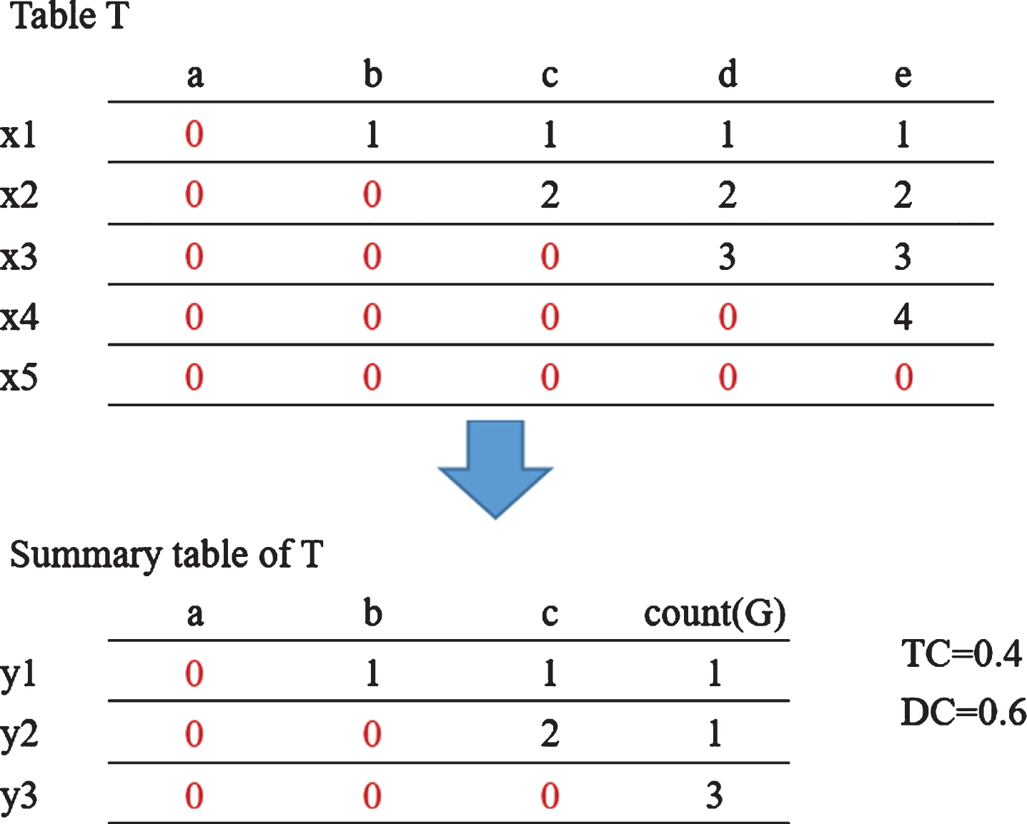
An example of a table and its summary table.

From the perspective of the summary table, our research is completely different from the previous attribute reduction studies A reduct is a subset of attributes that maintains the same indistinguishable relationship as the original table. It eliminates attributes that are considered to be dispensable, and the remaining attributes have 100% classification correctness. In other words, we keep a set of attributes that are indispensable to prevent any classification errors. On the other hand, the purpose of the summary table is to express the main content of our knowledge in a concise structure so that users can filter and search in a shorter time. The core concept of the summary table is still based on the indiscernibility relation of the Pawlak rough set theory. Attributes are divided into summary attributes and removed attributes, where the deleted attributes are called removed attributes and the remaining attributes are called summary attributes. However, the summary of the information system must consider two criteria: distortion and compression. Distortion represents the degree to which the data in the summary table is misclassified compared to the data in the original table. If the distortion is low, it means that the summary table is closer to the original knowledge. Compression is the degree to which the data in the summary table is reduced compared to the data in the originaltable.

The rest of this paper is organized as follows. Section 2 reviews some of the basic concepts of rough sets, including discernibility relation and the reduct of attributes. In Section 3, the definition of the summary table is given. Section 4 studies the distortion and compression in the summary table. Section 5 examines the relationship between distortion and compression and then proposes algorithms to obtain a satisfactory summary table. Conclusions follow in Section 6.

2 Preliminaries

2.1 Information systems

An information system is a pair T = (U, A), where U and A are finite nonempty sets called the universe and the set of attributes, respectively. With every attribute a ∈ A we associate a set V_a as its values, called the domain of a.

An information system can be viewed as a data table, consisting of objects (rows in the table) and attributes (columns). Table 1 is a simple example, where U = {x1,x2,x3,x4,x5} is a set of objects, and A = {a,b,c} is a set of attributes.

Table 1
An information system

a b c

x1 1 2 3

x2 1 2 3

x3 2 3 4

x4 2 3 4

x5 2 3 4

	a	b	c
x1	1	2	3
x2	1	2	3
x3	2	3	4
x4	2	3	4
x5	2	3	4

2.2 Indiscernibility relation

Indiscernibility relation is an important concept in rough set theory. Let T = (U, A) be an information system; then, with any B ⊆ A there is an associated indiscernibility relation: IND (B) ={ (x, x′) ∈ U² ∀ a ∈ B, a (x) = a (x′) }, where IND(B) is called the B-indiscernibility relation. If (x, x′) ∈ IND (B) then objects x and x′ are indiscernible from each other by attributes from B. Obviously, IND(B) is an equivalence relation.

The equivalence classes of the B-indiscernibility relation are denoted by [x] _B. A partition of U determined by B is all equivalence classes of IND(B), and is denoted by U/IND(B). An equivalence class of U/IND(B) is a granule of the partition U/IND(B).

2.3 Representatives of equivalence classes

Every two equivalence classes [x] and [y] in U/IND(B) are either equal or disjoint. This means that every object is in one and only one equivalence class. The intersection of two classes is empty and the union of all classes is the universe.

The representative of an equivalence class is a single object of that class. Let y ∈ [x] _B, then x is a representative of [x] _B. Any object of a class can be chosen as a representative of the class. A set of class representatives is a subset of U which contains exactly one object from each equivalence class.

For example, according to Table 1, let B be the full set of attributes. There are two equivalence classes in U/IND(B), which are {x1,x2} and {x3,x4,x5}. Let y1 be the representative of x1,x2 and y2 be the representative of {x3,x4,x5}. The set of class representatives is {y1, y2}. Table 2 is an example of representatives based on Table 1.

Table 2
A set of class representatives based on Table 1

a b c

y1 1 2 3

y2 2 3 4

	a	b	c
y1	1	2	3
y2	2	3	4

2.4 Reduct and core

Given an information system T = (U, A). Let B be a subset of A and let a belong to B. We say that a is dispensable in B if IND(B) = IND(B-{a}); otherwise a is indispensable in B.

A reduct of A is a minimal set of attributes B ⊆ A such that IND(B) = IND(A). In other words, a reduct is a minimal set of attributes from A that preserves the partition of the universe. Therefore, compared with using the entire attribute set A to classify, consistent results can be held by using reduct to classify.

The notion of a core of attributes is defined as follows. Let B be a subset of A. The core of B is the set of all indispensable attributes of B. The following function connects the notion of the core and the reducts.

Core (B) = ∩ Red (B), where Red(B) is the set of all reducts of B.

3 Problem definition

In this section, we formally introduce the research problem. In order to more accurately express the definition of the summary table, we need some auxiliary concepts.

A partition U/IND(B) is all equivalence classes; we call these granules. Each granule represents an equivalence class and is also a subset of U. Let $G_{i}^{B}$ be a granule of IND(B), $G_{i}^{B} \subseteq U$ . When the granules are generated from the same indiscernibility relation, superscripts can be ignored.

In the summary table, an attribute count (G_i) is added to denote the size of a granule G_i. For example, according to Table 1, the full set of attributes B = {a,b,c} is considered. There are two granules, G₁ and G₂, where G₁= {x1,x2} and G₂= {x3,x4,x5}. Thus, we have count (G₁) =2 and count (G₂) =3.

Let T = (U, A) be an information system, then with any B ⊆ A there is an associated indiscernibility relation. A summary table is denoted by ST (B) = (R, B ∪ { {count (G)} }), where R is a non-empty, finite set of representatives and B∪ { count (G) } is a non-empty, finite set of attributes such that a : R → V_a for every a∈ B ∪ { {count (G)} }. V_a is called the value set of a.

We call B the summary attribute set in the summary table. B is a set of attributes that must be retained in the summary table. Let B = A-C, and C is called the removed attribute set. The set C contains those attributes that are removed from A and are not used by the summary table. If A = B, it means that the summary table takes the entire information system attribute set as a summary attribute set. Therefore, the removed attribute set is empty. When removed attribute set C is empty, it can be considered as the initial summary table of the process. For example, according to Table 1, the entire set of attributes B = {a,b,c} is considered. The resulting summary table (in Table 3) is based on Table 1. Unlike Table 2, Table 3 has an additional attribute count (G), which is the size of each granule.

Table 3
An initial summary table

a b c count(G)

y1 1 2 3 2

y2 2 3 4 3

	a	b	c	count(G)
y1	1	2	3	2
y2	2	3	4	3

The other extreme case is that all the attributes in the original table are removed attributes, that is C = A or B =φ. This is the final summary table. C = A means that all the attributes in the original table are treated as removed attributes. The result is to treat the summary table as a granule, which is to turn knowledge into an abstract concept. Let us give an example. Table 4 is the final summary table based on Table 1. There is an additional attribute count(G), which is the size of the single granule y1.

Table 4

A final summary table

	count(G)
y1	5

According to the definition of the summary table, there will be many possibilities for summary attribute sets in the information system. Which combination of attributes is the best for a summary table? In the next section we will present some indicators as criteria for selecting summary attributes.

4 Methodology

In general, a summary table does not take the entire attribute set as the summary attributes. In this section, we consider the case B ⊂ A, where the removed attribute set is not empty. We divide this section into three subsections. The first is to review the important properties of the granules, and how granules change when certain attributes are removed. The last two subsections define the degree of compression and the degree of distortion, based on which we can measure the goodness of the summary table.

4.1 The change of granules

In the information system, the granules are generated from the indiscernibility relation. The equivalence relation creates the partition, in which each granule is an equivalence class.

Let T = (U, A) be an information system. For B ⊆ A, there is a B-indiscernibility relation. If the partition U/IND(B) has granules G₁, G₂, . . . , G_n, they have the following important properties:

Theorem 4.1.1. Let U be a nonempty set and let ∼ be an equivalence relation on the set U. Then,

For each a ∈ U, a ∈ G_a.

For each a, b ∈ U, a ∼ b if and only if G_a = G_b.

For each a, b ∈ U, G_a = G_b or G_a∩ G_b = ∅

Theorem 4.1.1 shows that every object of U is in its own granule, two objects are equivalent if and only if their granules are equal. In addition, two granules are either identical or they are disjoint. This means that if two granules are not disjoint then they must be equal.

In the process of summarizing the data table, the choice of attributes must be considered first. According to rough set theory, some attributes are dispensable, but there are also attributes that are indispensable. If we want to summarize a data table by removing some attributes, we must evaluate how important or how representative the attributes are. To this end, we consider the three possibilities for the states of granules. The three states are: unchanged granules, the granules split, and the granules merge. The following defines them each separately.

4.1.1 Granules remain unchanged

Let T = (U, A). There is an A-indiscernibility relation, and the partition U/IND(A) has granules G₁, G₂, . . . , G_n. Let T = (U, A), B ⊂ A. There is a B-indiscernibility relation, and the partition U/IND(B) has granules $G_{1}^{'}, G_{2}^{'}, . . ., G_{m}^{'}$ . We say granule G_iis unchanged if for any x ∈ G_i, we have $x \in G_{i}^{'}$ and count(G_i)=count( $G_{i}^{'}$ ). The unchanged granule represents that some part of the equivalent structures is invariant.

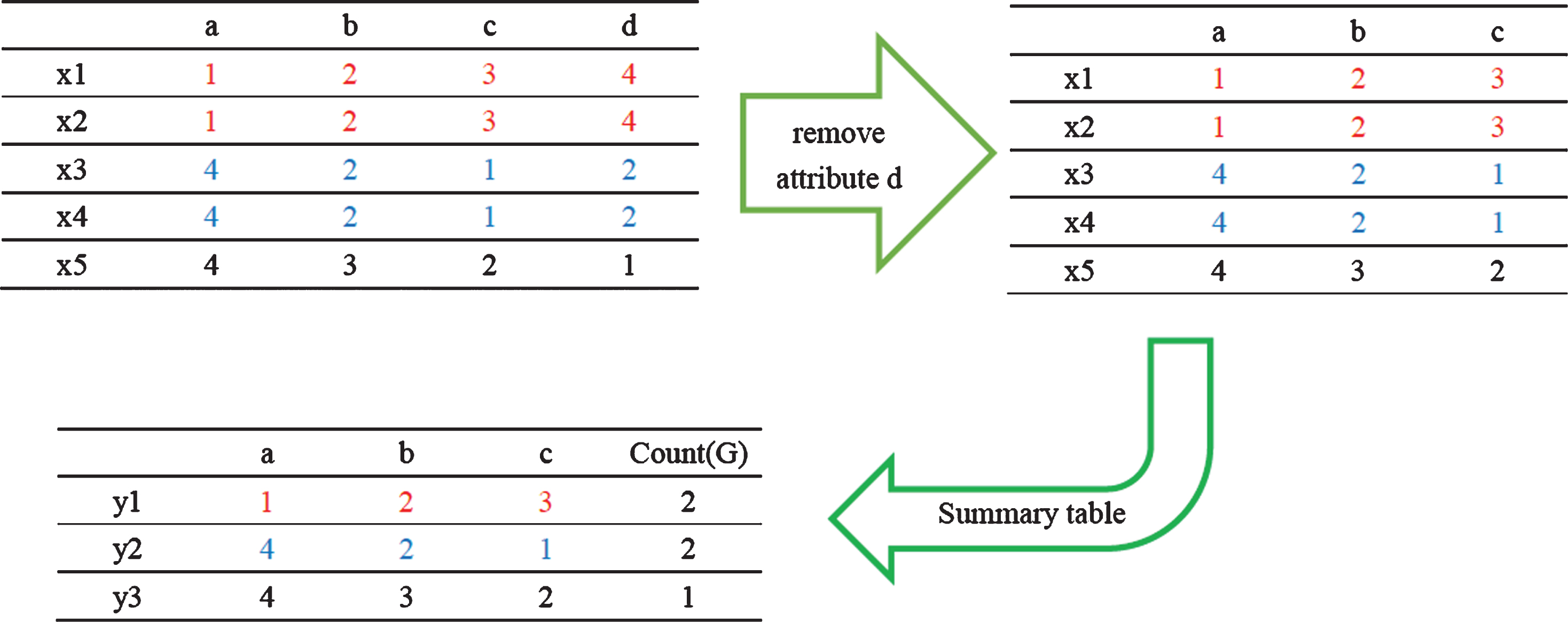
When any dispensable attribute is removed, all granules will be unchanged. There is a simple example in Fig. 2. A = {a,b,c,d}. If attribute d is removed, we get a new table which preserves the same partition. Therefore, each granule remains unchanged. G₁ = {x1,x2}= $G_{1}^{'}$ , G₂={x3,x4}= $G_{2}^{'}$ , G₃={x5}= $G_{3}^{'}$ , count(G₁)=count( $G_{1}^{'}$ )=2, count(G₂)=count( $G_{2}^{'}$ )=2, count(G₃)=count( $G_{3}^{'}$ )=1. We finally get a summary table with the summary attribute set B = {a,b,c}.

Fig. 2

An example of granules unchanged.

4.1.2 Granules split

Let T = (U, A). There is an A-indiscernibility relation. The partition U/IND(A) has granules G₁, G₂, . . . , G_n. Let T = (U, A), B ⊂ A. There is a B-indiscernibility relation. The partition U/IND(B) has granules $G_{1}^{'}, G_{2}^{'}, . . ., G_{m}^{'}$ . We say that granule G_iis split if there are two objects x ∈ G_i and y ∈ G_i, but they satisfy $x \in G_{i}^{'}, y \in G_{j}^{'}, G_{i}^{'} \neq G_{j}^{'}$ .

It is easy to show that a granule split cannot occur due to attribute removal. Each granule represents an equivalence class. Let us consider two objects x and y in G_i, x ∼ y, meaning that they have the same attribute values in granule G_i. If the granule splits, $x \in G_{i}^{'}, y \in G_{j}^{'}, G_{i}^{'} \neq G_{j}^{'}$ , but x ∼ y. This will lead to conflicting results with Theorem 4.1.1.

4.1.3 Granules merge

We consider the state of the last type of granule. Let T = (U, A). There is an A-indiscernibility relation. The partition U/IND(A) has granules G₁, G₂, . . . , G_n. Let T = (U, A), B ⊂ A. There is a B-indiscernibility relation. The partition U/IND(B) has granules $G_{1}^{'}, G_{2}^{'}, . . ., G_{m}^{'}$ . We say that granules G_iand G_jare merged if there are two objects x ∈ G_i and y ∈ G_j, G_i ≠ G_j, but they satisfy $x \in G_{i}^{'}, y \in G_{i}^{'}$

The merged granule represents that some parts of the equivalent structures have collapsed. This means that if the indispensable attributes in the table are removed, some granules will be merged.

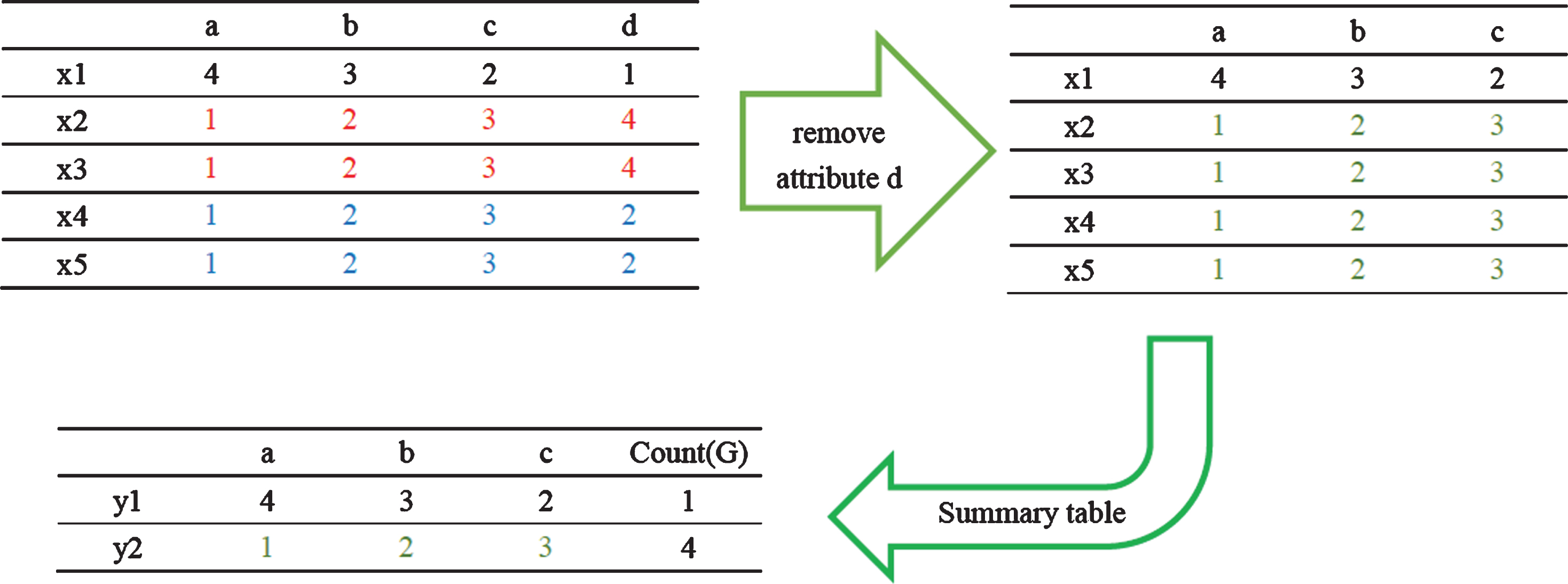
Figure 3 shows an example. G₁={x1}, G₂={x2,x3}, G₃={x4,x5}. If attribute d is removed from the table, $G_{1}^{'}$ =x1, $G_{2}^{'}$ ={x2, x3, x4, x5}, the objects in G₁and G₂are merged into a new granule $G_{2}^{'}$ . We finally get a summary table with the summary attribute set B = {a,b,c}

Fig. 3

An example of granules merge.

4.2 The degree of compression (DC)

The representatives of equivalence classes are regarded as objects of the summary table that produce a condensed or compressed effect. One purpose of the summarization is to reduce the amount of data stored, and make it visually simpler and easier to read.

Let T = (U, A), B ⊆ A, and ST (B) = (R, B ∪ { count (G) }) be a summary table. The degree of compression (DC) is presented as follows. $DC (B) = \frac{| R |}{| U |}$

|U| denotes the cardinality of objects and |R| denotes the cardinality of a set of representatives. |R| also represents the number of granules. The lower the DC value, the smaller the representative number, and the more simplified the summary table.

In the beginning, the summary table takes the entire attribute set of data table as a summary attribute set, and we can obtain the initial DC value. If some dispensable attributes are removed from the attributes set, all granules keep unchanged and the number of representatives are the same as those in the initial summary table. If some indispensable attributes are removed from the attributes set, granules will be merged. The total number of granules decreases, which means that DC becomes lower than the initial value.

4.3 The degree of distortion

Another metric about the summarization of the information system is the degree of distortion. It is caused by misclassification in the summary table. Distortion is considered to be a measure of similarity between the summary table and the original table. Many studies on attribute reduction in rough set theory have to maintain the consistency of classification results and avoid distortion. Our research is very different in this respect, because we allow a certain degree of misclassification (distortion) if we can compensate for this sacrifice through data summarization (data compression).

We continue to discuss the case when the removed attribute set is not empty. Exploring the distortion of the summary table compared to the initial table is an important topic. The detailed definitions of distortion are given in the following two subsections.

4.3.1 Granule classification error (GC)

Merging granules (indispensable attribute removal) is the reason why the table is distorted, so we can use information loss to measure the degree to which the structure is distorted. In the process of the summarization, if the granules are unchanged, the equivalent structure remains the same. It can be considered that there is no classification error, thus the GC value is 0. If some granules are merged into a new granule, the GC value is defined asfollows.

Let T = (U, A), and B ⊂ A. We have granules $G_{1}^{A}, G_{2}^{A}, . . ., G_{n}^{A}$ and have granules $G_{1}^{B}, G_{2}^{B}, . . ., G_{m}^{B}$ . In summary table ST(B), if granule $G_{k}^{B}$ is created by merging from $G_{1}^{A}, G_{2}^{A}, . . ., G_{j}^{A}$ , then $GC (G_{k}^{B}) = 1 - max (\frac{count (G_{i}^{A})}{count (G_{k}^{B})}), i = 1, \dots, j$ .

The following explains why we set the GC value in this way. Suppose that several granules are merged together. This means that we use a merged granule to represent all of these individual granules. This will cause a certain degree of information loss. If we need to guess its original content, one way to minimize erroneous guessing is to guess its missing attributes as the content of the child granule with the highest probability of occurrence. By doing so, we have the probability $max (\frac{count (G_{i}^{A})}{count (G_{k}^{B})})$ , i = 1, ... , j, to correctly restore the original content. As a result, the classification error rate becomes $1 - max (\frac{count (G_{i}^{A})}{count (G_{k}^{B})})$ , i = 1, ... , j.

According to this formula, the GC value is zero when granules are unchanged for all granules. This is consistent with what we started with. However, if some granules are merged into a new granule, the GC value is greater than zero.

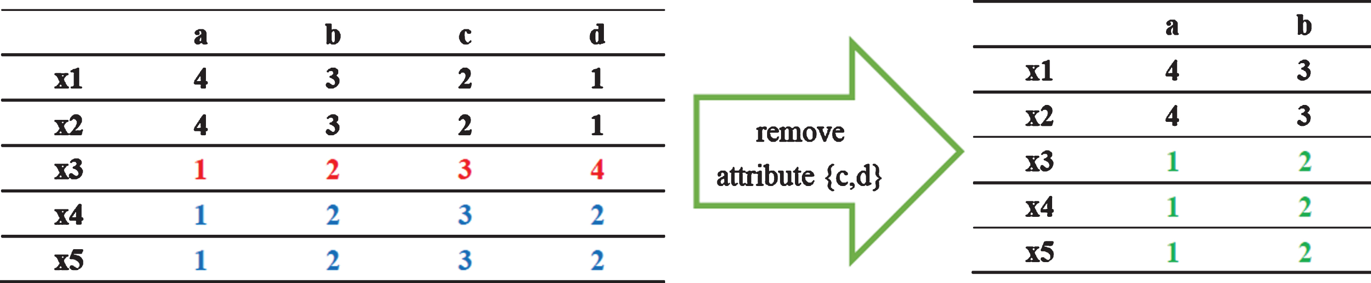
In Fig. 4, let A = {a,b,c,d}, B = {a,b}. We have granules $G_{1}^{A}$ ={x1,x2}, $G_{2}^{A}$ =x3, $G_{3}^{A}$ ={x4,x5}, $G_{1}^{B}$ ={x1,x2}, and $G_{2}^{B} = {x 3, x 4, x 5}$ . Therefore, GC( $G_{1}^{B}$ )=0 and GC( $G_{2}^{B}$ )=1-max(1/3,2/3) = 1-2/3 = 1/3.

Fig. 4

An example of GC.

4.3.2 Table classification error (TC)

Based on the classification errors of all the granules, we can define the table classification error rate. TC is the information loss of the summary table compared with the original table, and it can also be regarded as the indicator of similarity.

Let T = (U, A), and B ⊂ A. The table classification error is the weighted average of all GC values. The following is the formula: $\begin{matrix} TC (B) = \sum_{i} [\frac{count (G_{i}^{B})}{| U |} GC (G_{i}^{B})], i = 1, . . ., n . \end{matrix}$

According to this formula, the TC value is zero when all granules are unchanged. But if some granules are merged into a new granule, the TC value becomes greater than zero. In Fig. 4, we know that $GC (G_{1}^{B}) = 0$ and $GC (G_{2}^{B}) = 1 / 3$ . Therefore, TC(B) = 2/5×0 + 3/5×1/3 = 1/5.

The degree of compression (DC) and table classification error (TC) are two important indicators of the summarization. In summarization, we want less distortion and higher data compression. In other words, we prefer smaller TC values and smaller DC values. We need a summary table that meets these conditions. However, such a summary table will face some challenges to meet the aboverequirements.

In the following, we will explain the challenge of choosing a good summary table and then propose an algorithm to find a solution.

5 The relationship between distortion and compression

The reduct of attributes is an important concept in the rough set theory. If we choose the reduct of attributes as the summary attribute set, the indicator TC of the summary table will be zero, but the indicator DC will be a value between 0 and 1. By removing more attributes from the attribute set, the TC value will increase, but the DC value will decrease. Since we prefer smaller TC values and smaller DC values, we do not like the former effect, but prefer the latter. How to balance these two effects and find an efficient removed attribute set is an important issue to be studied. In this section, we will investigate the anti-monotone properties of DC and TC, and then propose algorithms to find all efficient sets.

5.1 Reduct

A reduct is a minimal set of attributes in the table such that it maintains the same partition. In other words, a reduct is a minimal set of attributes from the entire attribute set that preserves the partitioning of the universe.

Consider the reduct as the summary attribute set. Assume that B is a reduct of A and B ⊂ A. Let the degree of compression DC(A) = t be the initial DC value. Then DC(A) = DC(B)=t, because none of the granules are merged. This means that all reducts have the same DC value as the initial value.

By the same reasoning, TC(A) = 0. If B is a reduct of A, then TC(B) = 0. Since none of the granules have been merged, this means that the TC values of all reducts are zero, which implies that there is no classification error.

If the summary table only uses the reduct as the summary attribute set, the two indicators DC and TC are the same as the initial summary table. Such a summary table is not the best option. Although the degree of distortion is low, the degree of compression should be further improved.

5.2 The general property of TC and DC

Let T = (U, A), a_m and a_n be the removed attributes, and C and D be the removed attribute sets. There are four properties related to TC.

Property 5.2.1. If all the granules are unchanged when we remove {a_m} from the initial summary table ST(A), then TC (A - {a_m}) = 0.

Property 5.2.2. If some granules are merged when we remove {a_m} from the initial summary table ST(A), then TC (A - {a_m}) > 0.

This is because GC > 0 when some granules are merged. Thus the TC value must be greater than zero.

Property 5.2.3. If TC (A - {a_m}) = b, and TC (A - {a_m}) = c, then TC (A - { a_m ∪ a_n }) ⩾ max(b, c).

Proof: Let the summary attribute set B = A-{a_m}, then A - {a_m ∪ a_n} = B - a_n. If all the granules are unchanged, according to Property 5.2.1, TC (A - { a_m ∪ a_n }) = TC (B - a_n) = b + 0 = b. Otherwise, if some granules are merged, according to Property 5.2.2, TC (A - { a_m ∪ a_n }) = TC (B - a_n) > b. We therefore prove that TC(A- {a_m ∪ a_n})≥b.

For the same reason, TC(A- {a_m ∪ a_n})≥c can be proved. Finally we have TC(A-{a_m ∪ a_n})≥max(b,c).

Property 5.2.4. If removed attribute set C ⊂ D and TC(A-C) = d, then TC(A-D)≥d.

We can use similar reasoning as property 5.2.3 to get this result.

There are also four properties related to DC.

Property 5.2.5. If all the granules are unchanged when we remove {a_m} from the initial summary table ST(A), then DC(A-{a_m})=DC(A).

Property 5.2.6. If some granules are merged when we remove {a_m} from the initial summary table ST(A), then DC(A- {a_m})<DC(A).

Since the granules are merged, the number of granules in the entire table reduces and the number of representatives also decreases, so the DC value will become smaller.

Property 5.2.7. If DC(A - {a_m})=b and DC(A- {a_n})=c, then DC(A- {a_m ∪ a_n})≤min(b,c).

Property 5.2.8. If removed attribute set C ⊂ D and DC(A-C) = d, then DC(A-D)≤d.

We can use the similar reasoning as property 5.2.3 to prove Property 5.2.7 and Property 5.2.8. We therefore skip these proofs. Here, we use Fig. 5 to show an example of how the original table can be summarized in different ways by using different removed attributes. In this example, we also show how the values of DC and TC change for different summary tables. It can be seen that as more attributes are removed, DC will decrease but TC will increase. Since DC and TC are opposite, the attribute removal process must stop at some point where the TC value is acceptable.

Fig. 5

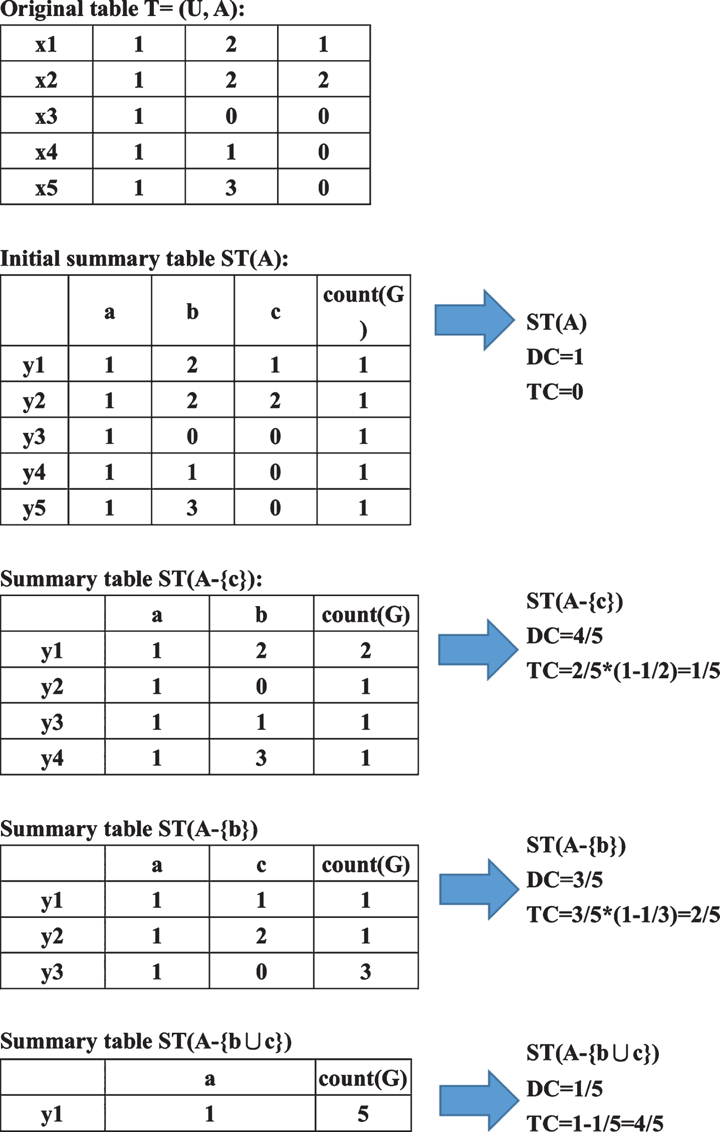
Example of different combinations of removed attributes.

A good summary table should have the least distortion and also have a high data compression. In other words, we require a smaller TC value and a smaller DC value. However, when the size of the removed attribute set changes, the degree of distortion and the degree of compression have the opposite result. Therefore, we propose a compromise method to solve the dilemma, i.e., how to choose a good summary table for the information system.

5.3 Maximal removed attribute set and algorithm

We use formal mathematics to describe and analyze this problem. Let p be the upper bound of the information distortion, TC≤p.

Definition 5.3.1. A removed attribute set C is called feasible if it satisfies the threshold of the distortion, TC (A - C) ≤ p.

Let X = {X₁, X₂, . . . , X_m} be the set of all feasible removed attribute sets, i.e, we have a family of removed attribute sets in X. There is a smaller family of feasible removed attribute sets in X which we said is maximal and can be defined as follows.

Definition 5.3.2. A feasible removed attribute set C is maximal if none of its immediate superset, D, satisfies TC (A - D) ≤ p.

When a removed attribute set C is maximal, it means we cannot add any further attribute to this set. Otherwise, it will cause a violation of the TC constraint. Let y = {Y₁, Y₂, . . . , Y_n} be the set of all maximal removed attribute sets. Obviously, Y is a subset of X.

Theorem 5.3.1. The DC value of a maximal removed attribute set is smaller or equal to any of its subsets.

According to the property 5.2.8, for any subset of a maximal removed attribute set, its DC value is greater or equal to that of the maximal removed attribute set. Therefore, the maximal removed attribute set has smaller DC value than its subsets.

Theorem 5.3.2. A removed attribute set C is optimal if it satisfies TC≤p and has the smallest DC value. This optimal set C must exist in the maximal removed attribute set Y.

If a removed attribute set is not in Y, it is either not feasible or has some supersets in Y with smaller DC values. Therefore, the optimal removed set must be in Y.

From the above two theorems, it is very important to find a cover of maximal removed attribute sets when selecting a good summary table. Next, two algorithms were developed to find the feasible and maximal removed attribute sets. Let us explain the operation of the algorithms and give a simpleexample.

Let p be the upper bound value of distortion degree. Then TC≤p can be used as the constraint to select the summary table. Intuitively, all subsets of attributes must be tested to find whether the constraint is satisfied. However, according to Property 5.2.4, when C is a subset of D, if TC (A-C) does not meet the constraint then TC (A-D) does not meet the constraint either. This is called the anti-monotone property. Property 5.2.8 shows that DC also has the anti-monotone property. Designing an algorithm based on the anti-monotone property can greatly reduce the computation time and achieve better efficiency. Since we summarize the table from the perspective of the distortion degree, the purpose of Algorithm 1 is to obtain a set of feasible removed attribute sets that satisfy the constraint TC≤p. Then, from these feasible removed attribute sets, we design Algorithm 2 to find a set of summary tables based on the maximal removed attribute sets. Finally, we can select the optimal removed attribute set from the maximal set.

Algorithm 1
1 Let TC denote the table classification error
2 Let C_k denote the set of removed attribute sets of size k
3 k = 1
4 Find all C₁satisfying TC≤p
5 Repeat
6 k = k+1
7 generate candidates in C_kby joining all pairs of feasible
sets in C_k-1
8 prune candidates in C_kcontaining subsets not in C_k-1
9 compute TC for each candidate in C_k
10 eliminate the candidates in C_kwhich do not meet TC≤p
11 Until C_k =∅

Theorem 5.3.3. The time complexity of Algorithm 1 is O(m^k+2n), where m is the number of attributes, n is the number of tuples in a table, and K is the total number of phases performed in the algorithm.

Proof. In the first phase, we will generate C₁ which contains all attributes satisfying TC ≤ p. To find them, we must examine the entire table for each attribute row by row; therefore, the time required is O (m × (m × n)) = O (m²n). Then, we must generate C₂ from C₁. Because the size of C₁ may be equal to O (m) in the worst case, the size of C₂ can be equal to O (m²). To determine whether these sets in C₂ satisfy the TC constraint, we must check the entire table row by row for each set in C₂; therefore, the time needed is O (m² × (m × n)) = O (m³n). Repeat this until phase K; our total time complexity in the worst case is O (m²n) + O (m³n) + … + O (m^k+1n) = O (m^k+2n).

We use a simple example to illustrate how these two algorithms work. Algorithm 1 is an iterative method. Suppose a table T has a set of attributes A = {a, b, c, d, e, f, g}, and TC≤p is the constraint of the summary table. If a removed attribute set satisfies TC ≤ p, it is feasible, otherwise it is infeasible. C_k represents the feasible removed sets with k attributes (size is k).

Step 3 and step 4 is a method of generating the removed attribute sets of size 1. The candidate removed attribute sets of size 1 are listed first, and then whether these sets satisfy the criterion of TC ≤ p is calculated. As shown in Fig. 6, from the 6 candidate sets, 5 sets of calculation results are feasible, namely sets {a}, {b}, {c}, {d}, and {e}. These removed attribute sets constitute C₁.

Fig. 6

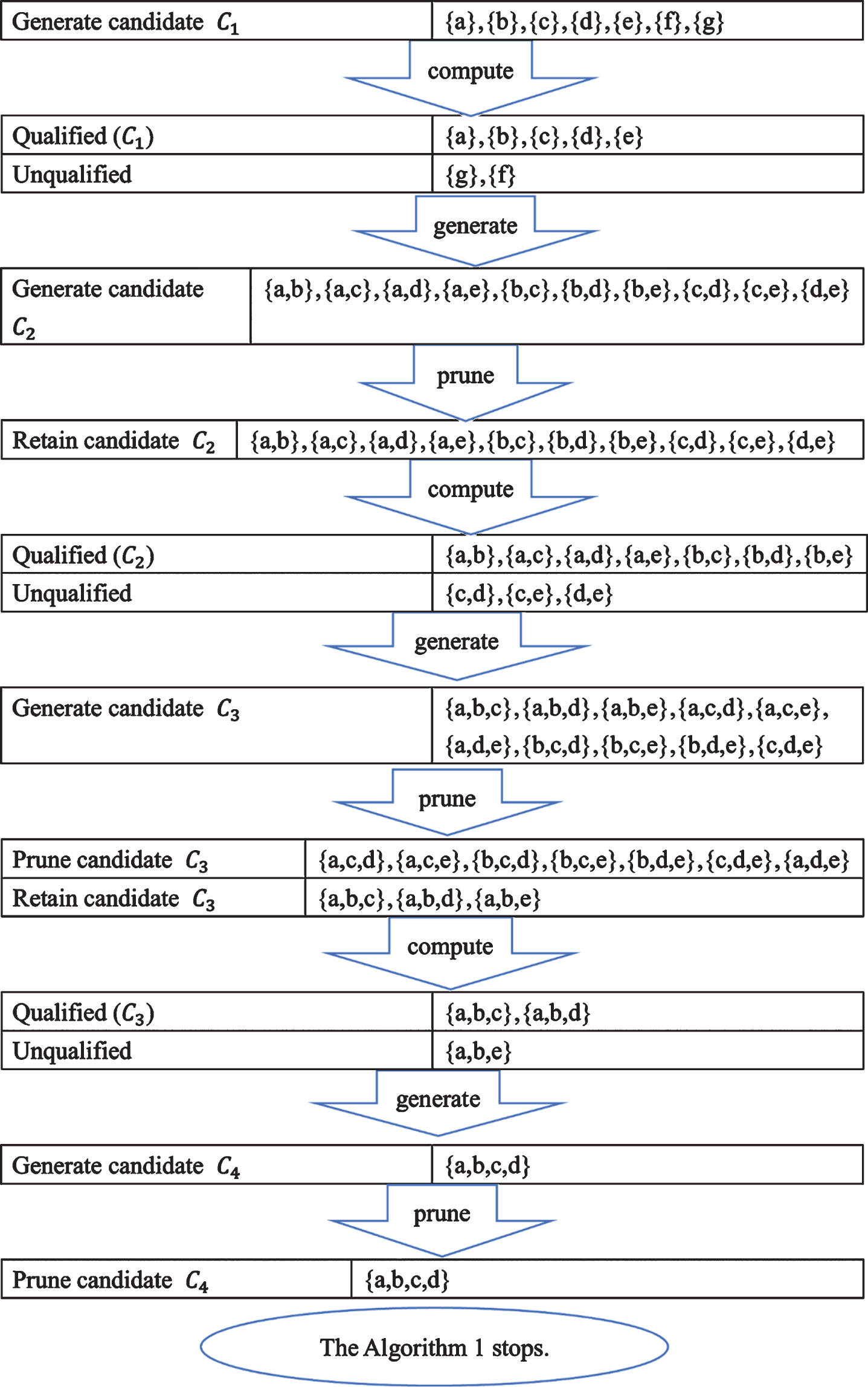
An example for illustrating Algorithm 1.

In Algorithm 1, steps 6 to 10 are methods for generating C_k. Let us first explain how to generate C₂. As shown in Fig. 6, ten candidate removed attribute sets of size 2 can be generated by combining any two sets of C₁. Next, each attribute set in C₂ is checked to see whether it contains a subset that is not in C₁. Since the subsets of these 10 sets all come from C₁, they are all retained. Finally, we calculate whether these sets meet the criterion of TC ≤ p. From the 10 candidate sets, there are 7 feasible sets, which are {a,b}, {a,c}, {a,d}, {a,e}, {b,c}, {b,d}, and {b,e}. These are the feasible removed attribute sets in C₂.

The method that produces C₃ is similar to the generation of C₂. In Fig. 6, 10 candidate removed attribute sets of size 3 can be generated by combining any two sets of C₂. Next, each attribute set in C₃ is checked to see whether it contains a subset that is not in C₂. As a result of the check, we prune 7 candidates in C₃, and 3 candidates in C₃ are kept. For example, the set {a, c, d} contains the subsets {c, d}. According to the anti-monotone property, if TC(A-{c, d}) does not meet the constraint, then TC(A-{a, c, d}) does not meet the constraint either. So the set a, c, d must be pruned. Finally, we calculate whether these sets meet the criterion of TC≤p. In the 3 candidate sets, there are 2 feasible sets, which are {a,b,c} and {a,b,d}. These are the feasible removed attribute sets C₃.

Step 11 is the stop condition of algorithm 1. When the removed attribute set can no longer be generated, Algorithm 1 will stop. As shown in Fig. 6, although a candidate removed attribute set of size 4 is generated, {a, b, c, d} contains the infeasible subset {b, c, d}, so it must be pruned. Then Algorithm 1 was stopped.

Algorithm 2
1 Let K_max denote the maximum size of feasible removed
attribute sets
2 Let C_kdenote the set of feasible removed attribute sets
of size k
3 Let DC denote the degree of compression
4 For k = K_max down to 1 do
5 For each feasible attribute set in C_k
6 remove all subsets of the attribute set
7 end for
8 compute DC values for the remaining attribute sets in C_k
9 Select the removed attribute set with the smallest DC value

The core concept of Algorithm 2 is to remove all subsets of the maximal removed attribute set. This is also based on the anti-monotone property of the DC value. According to Property 5.2.8, if removed attribute set C ⊂ D and DC(A-D) = d, then DC(A-C) ≥d. This means that the DC value of the subset is never smaller than the parent set.

Theorem 5.3.4. The time complexity of Algorithm 2 is O (Cmn + C²), where $C = \sum_{i = 1}^{K} | C_{i} |$ , m is the number of attributes, n is the number of tuples in a table, and K is the he maximum size of feasible removed attribute sets.

Proof. In Algorithm 2, we first remove all attribute subsets from C_K to C₁. This can be done by checking whether the smaller size attribute set is included in the larger size attribute set. Because there are a total of C² pairs of attribute sets, it can be completed in O(C²) time. After completing this operation, we must compute the DC value for each remaining attribute set. To find them, we must check each remaining attribute set in the entire table row by row; therefore, the time required is O (C × (m × n)) = O (Cmn). Finally, we must find the attribute set with the smallest DC value, which can be done in time of O(C). Adding the time for these three operations together, we get the worst case total time complexity as O(Cmn + C²).

We use the example of Algorithm 1 to continue the illustration of Algorithm 2. According to the result of Algorithm 1, a set of feasible removed attribute sets can be obtained, as shown in Table 5. In Algorithm 2, it first finds that K_maxis 3 and the set of C₃ is {a, b, c}, {a, b, d}. The subsets of C₃, which are {a,b},{a,c},{a,d},{b,c},{b,d},{a},{b},{c}, and {d}, can be removed, because their DC values are at least as large as those of {a, b, c} and {a, b, d}. The results are shown in Table 6. Next, it continues to find k = 2, and the sets of C₂ are {a, e} and {b, e}. A subset of C₂, {e}, can be removed. The results are shown in Table 7. Finally, it no longer finds smaller size removed attribute sets, so the algorithm stops searching and collects the remaining removed attribute sets to calculate their DC values. The maximal removed attribute sets we get according to Table 7 are {a,e},{b,e},{a,b,c}, and {a,b,d}. We calculate the DC of these sets. Finally, we choose the set with the smallest DC value.

Table 5

Feasible removed attribute sets obtained from Algorithm 1

C ₁	{a},{b},{c},{d},{e}
C ₂	{a,b},{a,c},{a,d},{a,e},{b,c},{b,d},{b,e}
C ₃	{a,b,c},{a,b,d}

Table 6

The results after removing subsets in C₃

C ₁	{e}
C ₂	{a,e},{b,e}
C ₃	{a,b,c},{a,b,d}

Table 7

The results after removing subsets in C₂

C ₁	∅
C ₂	{a,e},{b,e}
C ₃	{a,b,c},{a,b,d}

Here, we want to compare the two algorithms. Basically, their purpose is different. The purpose of Algorithm 1 is to obtain a set of feasible removed attribute sets satisfying the constraint TC ≤ p. On the other hand, Algorithm 2 is to find the summary table with the smallest DC value from these feasible removed attribute sets. In other words, Algorithm 1 is to obtain a set of feasible solutions from the input table, but Algorithm 2 is to find the optimal solution from all these feasible sets obtained from Algorithm 1. Another difference between the two algorithms is that Algorithm 1 uses the TC criterion to find feasible solutions, while Algorithm 2 uses the DC criterion to obtain the optimal solution. In other words, Algorithm 1 is to generate the set of feasible solutions that satisfy the constraint, whereas Algorithm 2 is to find the optimal solution with the minimum objective value.

Our proposed algorithm has several merits. First of all, this is the first work to summarize the information table based on the distortion criterion and compression ratio criterion. This opens up a new research route for many potential future studies in summarization based on rough sets. Second, the anti-monotone property used when building C_i from C_i-1 can help reduce the size of C_i, thereby improving the performance of Algorithm 1. Third, Algorithm 1 further reduces the size of C_i by deleting those candidate attribute sets that have any subsets not in C_i-1. This can also help improve the performance. Fourth, Algorithm 2 also removes all subsets of the maximal removed attribute set based on the anti-monotone property of the DC value. This can help quickly remove inefficient removed attribute sets and improve performance.

Let us take an experiment to further analyze the change of DC and TC values as the size of the removed attribute set grows larger. We use matlab tools to generate a synthetic table of the discrete uniform distribution integers. This random table is used as an information system. It has 200 objects, 20 attributes, and the values of the attributes are {1, 2, 3}.

In Fig. 7, the horizontal axis of the coordinates is the size of the set of removed attributes, and the vertical axis is the maximum value of the distortion TC corresponding to the set, expressed as a percentage. When the number of removed attributes increases, the value of TC increases. The results show that TC is a monotonic nondecreasing function. In Fig. 8, the horizontal axis of the coordinates is the size of the set of removed attributes, and the vertical axis is the minimum value of the compression DC corresponding to the set, expressed as a percentage. When the number of attributes increases, the value of DC decreases. The results show that DC is also a monotonic function which is entirely nonincreasing.

Fig. 7

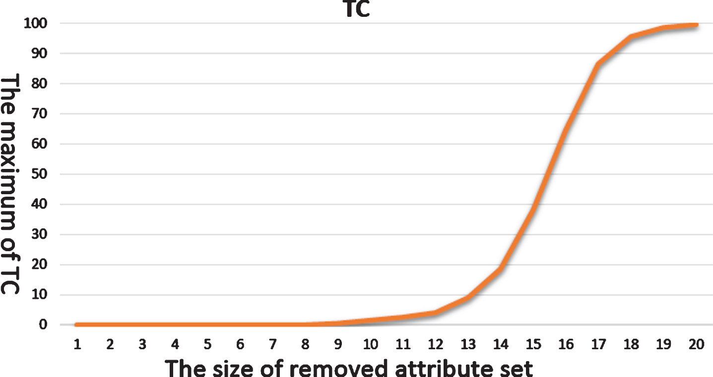
The maximum value of TC for different sizes of removed attribute sets.

Fig. 8

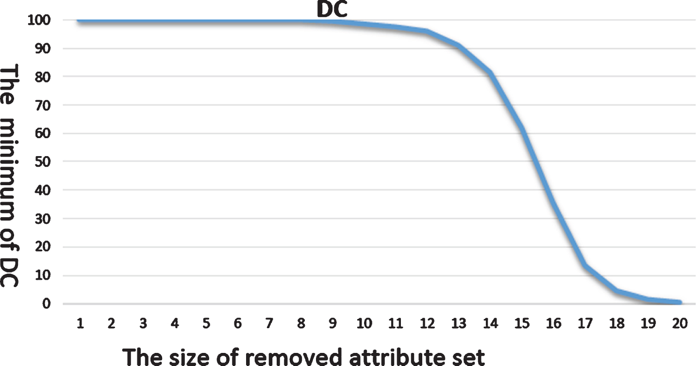
The minimum value of DC for different sizes of removed attribute sets.

When the number of removed attributes is less than 9, the table remains the same size and no distortion error occurs. Thus, these attribute are dispensable attributes. When the size of the removed attribute set is larger than 10, we see that the table size begins to reduce and the distortion error begins to increase. When the size of the removed attribute set is 14, the maximum TC is 18% and the minimum DC is 80%. When the size of the removed attribute set is 15, the maximum TC is 30% and the minimum DC is 60%. The former can reduce the table size by 20%, while the latter can reduce the table size by 40%. These two possibilities are reasonable choices that we can select. We can select the one that best meets our requirement.

6 Conclusions

The definition of the summary table is based on the indiscernibility relation of Pawlak’s rough set theory. In the summarization of the information system, we use two metrics as indicators. One is distortion, and the other is compression. The former refers to the extent to which the equivalent structure in the summary table is distorted compared to the original structure. The latter refers to the ratio of the number of representative elements in the summary table and that in the original table. A satisfactory summary table must satisfy the upper bound constraint on the distortion, and possess the best compression (smallest DC value).

The purpose of the summary table is to present the main content of knowledge in a concise structure so that users can filter and search in the shortest amount of time. Although we can choose reduct as summary attributes, such a summary table will not have any distortion, but will come at the expense of a larger table. In order to make the table more concise, it is reasonable to allow a certain degree of distortion. Based on this idea, we propose a summarization algorithm. The study also investigated the properties of distortion and compression.

We believe that the studies of summarization and attribute reduction are very different. Attribute reduction is finding the smallest subset of attributes that can achieve the same classification as the entire attribute set. It will produce a table without distortion and compression. Instead, this article seeks to compress tables. Therefore, we allow some degree of distortion that represents the similarity between the summary table and the original knowledge. Then, we present a summarization process that finds all the summary tables satisfying the distortion constraint. Finally, from these tables, we find the summary table with the best compression ratio.

There are several interesting directions for our research topics in the future. The first is to study how to measure the similarity between tables based on indistinguishable relations. Many studies on similarity measures are based on quantitative values in the table. The challenge is how to compare two or more tables when the values in the table are qualitative. We believe that from the perspective of the summary table, a way to compare tables with different qualitative values can be developed.

The second research topic is the conceptualization of knowledge. We can try to use the concept table to represent the conceptualization of knowledge. It is based on the fact that certain attributes can be grouped together into a common concept or theme. For example, eyes, ears, nose, mouth and eyebrows (attributes) can be abstracted into so-called “facial features” (themes). Distortion can also result when some properties are drawn into a common theme. A concept table is another form of simplifying knowledge. The conceptualization of the form will be interesting and deserves further study.

Finally, in all aspects of the attribute reduction research, we are looking for inspiration to simplify tables, for example, research topics on data uncertainty. How can we summarize this type of table when the data is incomplete or the data changes dynamically over time? In these cases, it is important to find the correct definition of distortion and compression. We can distort the table to some extent, and then obtain a summary table with the best compression results.

References

Azam

and Yao

, Game-theoretic rough sets for recommender systems, Knowledge-Based Systems 72 (2014), 96–107.

Chen

and Zhao

, Local reduction of decision system with fuzzy rough sets, Fuzzy Sets and Systems 161 (2010), 1971–1883.

Chen

, Zhang

, Wang

and Liu

, Uncertainty learning of rough set-based prediction under a holistic framework, Information Sciences 463-464 (2018), 129–151.

Chen

, Zhu

and Xu

, Finding rough set reducts with fish swarm algorithm, Knowledge-Based Systems 81 (2015), 22–29.

Chen

, Miao

and Wang

, A rough set approach to feature selection based on ant colony optimization, Pattern Recognition Letters 31 (2010), 226–233.

Eskandari

and Javidi

M.M.

, Online streaming feature selection using rough sets, International Journal of Approximate Reasoning 69 (2016), 35–57.

Fan

T.F.

, Liau

C.J.

and Liu

D.R.

, Dominance-based fuzzy rough set analysis of uncertain and possibilistic data tables, International Journal of Approximate Reasoning 52 (2011), 1283–1297.

Hamouda

S.K.M.

, Wahed

M.E.

, Abo Alez

R.H.

and Riad

, Robust breast cancer prediction system based on rough set theory at National Cancer Institute of Egypt, Computer Methods and Programs in Biomedicine 153 (2018), 259–268.

, Wang

, Huang

and Wu

. Incremental attribute reduction based on elementary sets, in: Proceedings of International Conference on Rough Sets, Fuzzy Sets, Data Mining, and Granular-Soft Computing, Berlin, Heidelberg, 2005, pp. 185–193.

10.

Huang

, Wang

H.H.

, Liu

and Wang

, Image de-noising and enhancement based on rough set and principal component analysis, in Proceedings of International Conference on Inventive Computing and Informatics (ICICI), 2017, pp. 536–539.

11.

Nguyen

H.S.

and Ślęzak

, “Approximate reducts and association rules,” in International Workshop on Rough Sets, Fuzzy Sets, Data Mining, and Granular-Soft Computing, 1999, pp. 137–145.

12.

Jothi

and Inbarani

, Hybrid tolerance rough set–firefly based supervised feature selection for mri brain tumor image classification, Applied Soft Computing 46 (2016), 639–651.

13.

Kryszkiewicz

, Rough set approach to incomplete information systems, Information Sciences 112 (1998), 39–49.

14.

Lin

, Li

, Wang

and Chen

, Attribute reduction for multi-label learning with fuzzy rough set, Knowledge-Based Systems 152 (2018), 51–61.

15.

, Qin

, Zhang

and Fang

, A fast feature selection approach based on rough set boundary regions, Pattern Recognition Letters 36 (2014), 81–88.

16.

X.M.

and Liang

, Application of rough set theory in coal gangue image process, in Proceedings of Fifth International Conference on Information Assurance and Security, 2009, pp. 87–90.

17.

Meng

and Shi

, Extended rough set-based attribute reduction in inconsistent incomplete decision systems, Information Sciences 204 (2012), 44–69.

18.

J.-S.

, Wu

W.-Z.

and Zhang

W.-X.

, Approaches to knowledge reduction based on variable precision rough set model, Information Sciences 159 (2004), 255–272.

19.

Miao

, Zhao

, Yao

, Li

and Xu

, Relative reducts in consistent and inconsistent decision tables of the Pawlak rough set model, Information Sciences 179 (2009), 4140–4150.

20.

Pawlak

and Skowron

, Rudiments of rough sets, Information Sciences 177 (2007), 3–27.

21.

Pawlak

, Rough sets and intelligent data analysis, Information Sciences 147 (2002), 1–12.

22.

Pawlak

, AI and intelligent industrial applications: the rough set perspective, Cybernetics and Systems 31 (2000), 227–252.

23.

Pawlak

, Rough set approach to knowledge-based decision support, European Journal of Operational Research 99 (1997), 48–57.

24.

Pawlak

, Rough Sets: Theoretical Aspects of Reasoning about Data, vol. 9, Springer Science & Business Media, 1991.

25.

Pawlak

, Rough sets, International Journal of Computer & Information Sciences 11 (1982), 341–356.

26.

Pawlak

and Sowinski

, Rough set approach to multi-attribute decision analysis, European Journal of Operational Research 72 (1994), 443–459.

27.

Qian

, Liang

, Wang

, Liang

, Liu

, Skowron

, Yao

, Ma

and Dang

, Local rough set: a solution to rough data analysis in big data, International Journal of Approximate Reasoning 97 (2018), 38–63.

28.

Qian

, Liang

, Li

, Wang

and Ma

, Approximation reduction in inconsistent incomplete decision tables, Knowledge-Based Systems 23 (2010), 427–433.

29.

Qiang

, Wei-jun

, Xin-ping

and Xuan

, Enhancement method for infrared dim-small target images based on rough set, in Proceedings of 4th International Conference on Information Science and Control Engineering (ICISCE), 2017, pp. 301–306.

30.

Raza

M.S.

and Qamar

, A heuristic based dependency calculation technique for rough set theory, Pattern Recognition 81 (2018), 309–325.

31.

Salvatore

, Matarazzo

and Slowinski

, Rough sets theory for multicriteria decision analysis, European Journal of Operational Research 129 (2001), 1–47.

32.

Skowron

and Rauszer

, The Discernibility Matrices and Functions in Information Systems, in Intelligent Decision Support: Handbook of Applications and Advances of the Rough Sets Theory, R. Słinowiński, Ed., ed Dordrecht: Springer Netherlands, 1992, pp. 331–362.

33.

Song

, Tsang

E.C.C.

, Chen

and Yang

, Minimal decision cost reduct in fuzzy decision-theoretic rough set model, Knowledge-Based Systems 126 (2017), 104–112.

34.

Sun

, Ma

, Li

and Li

, Three-way decisions approach to multiple attribute group decision making with linguistic information-based decision-theoretic rough fuzzy set, International Journal of Approximate Reasoning 93 (2018), 424–442.

35.

Suo

, An

, Zhou

and Li

, Grid-clustered rough set model for self-learning and fast reduction, Pattern Recognition Letters 106 (2018), 61–68.

36.

Susmaga

and Slowinski

, Generation of rough sets reducts and constructs based on inter-class and intra-class information, Fuzzy Sets and Systems 274 (2015), 124–142.

37.

Tan

, Wu

W.Z.

, Li

J.J.

and Lin

, Evidence-theory-based numerical characterization of multigranulation rough sets in incomplete information systems, Fuzzy Sets and Systems 294 (2016), 18–35.

38.

Wang

, Yang

, Teng

, Xia

and Jensen

, Feature selection based on rough sets and granule swarm optimization, Pattern Recognition Letters 28 (2007), 459–471.

39.

Wei

, Wu

, Liang

, Cui

and Sun

, Discernibility matrix based incremental attribute reduction for dynamic data, Knowledge-Based Systems 140 (2018), 142–157.

40.

Wroblewski

. Finding minimal reducts using genetic algorithms, in: Proccedings of the Second Annual Join Conference on Infromation Science, 1995, pp. 186-189.

41.

W.-Z.

, Attribute reduction based on evidence theory in incomplete decision systems, Information Sciences 178 (2008), 1355–1371.

42.

Yang

, Yang

, Wu

and Yu

, Dominance-based rough set approach and knowledge reductions in incomplete ordered information system, Information Sciences 178 (2008), 1219–1234.

43.

Yang

Y.Y.

, Chen

, Wang

, Tsang

E.C.C.

and Zhang

D.L.

, Fuzzy rough set based incremental attribute reduction from dynamic data with sample arriving, Fuzzy Sets and Systems 312 (2017), 66–86.

44.

Zhan

, Liu

and Herawan

, A novel soft rough set: Soft rough hemirings and corresponding multicriteria group decision making, Applied Soft Computing 54 (2017), 393–402.

45.

Zhan

, Jiang

and Yao

, Covering-based variable precision fuzzy rough sets with PROMETHEE-EDAS methods, Information Sciences 538 (2020), 314–336.

46.

Zhang

, Mei

, Chen

and Li

, Feature selection in mixed data: A method using a novel fuzzy rough set-based information entropy, Pattern Recognition 56 (2016), 1–15.

47.

Zhang

, Zhan

and Wang

, TOPSIS-WAA method based on a covering-based fuzzy rough set: an application to rating problem, Information Sciences 539 (2020), 397–421.

48.

Zhang

, Zhan

and Wu

W.Z.

, On multi-criteria decision-making method based on a fuzzy rough set model with fuzzy α-neighborhoods, IEEE Transactions on Fuzzy Systemsα (2020), 1–15.

49.

Zhang

, Wang

, Li

, He

and Sun

. A new heuristic reduct algorithm base on rough sets theory, in: Proceedings of International Conference on Web-Age Information Management, Berlin, Heidelberg, 2003, pp. 247–253.

50.

Zhang

, Mei

, Chen

and Yang

, A fuzzy rough set-based feature selection method using representative instances, Knowledge-Based Systems 151 (2018), 216–229.

51.

Zeng

, Li

T.R.

, Liu

, Zhang

J.B.

and Chen

H. M.

, A fuzzy rough set approach for incremental feature selection on hybrid information systems, Fuzzy Sets and Systems 258 (2015), 39–60.

52.

Zhong

, Dong

and Ohsuga

, Using Rough Sets with Heuristics for Feature Selection, Journal of Intelligent Information Systems 16 (2001), 199–214.

53.

Zhu

, Jing

and Chen

, A novel image retrieval model based on semantic information and probability rough set analysis method, in Proceedings of 2nd Asia-Pacific Conference on Intelligent Robot Systems (ACIRS), 2017, pp. 23–27.

54.

Ziarko

, Variable precision rough set model, Journal of Computer and System Sciences 46 (1993), 39–59.

Summarization of information systems based on rough set theory

Abstract

Keywords

1 Introduction

2.1 Information systems

Table 1 An information system a b c x1 1 2 3 x2 1 2 3 x3 2 3 4 x4 2 3 4 x5 2 3 4

2.3 Representatives of equivalence classes

Table 2 A set of class representatives based on Table 1 a b c y1 1 2 3 y2 2 3 4

3 Problem definition

Table 3 An initial summary table a b c count(G) y1 1 2 3 2 y2 2 3 4 3

4.1 The change of granules

4.1.1 Granules remain unchanged

4.1.3 Granules merge

4.3 The degree of distortion

4.3.1 Granule classification error (GC)

5 The relationship between distortion and compression

5.1 Reduct

5.2 The general property of TC and DC

References

Table 1
An information system

a b c

x1 1 2 3

x2 1 2 3

x3 2 3 4

x4 2 3 4

x5 2 3 4

Table 2
A set of class representatives based on Table 1

a b c

y1 1 2 3

y2 2 3 4

Table 3
An initial summary table

a b c count(G)

y1 1 2 3 2

y2 2 3 4 3