Personalized travel route recommendation algorithm based on improved genetic algorithm

Abstract

The analysis of user trajectory information and social relationships in social media, combined with the personalization of travel needs, allows users to better plan their travel routes. However, existing methods take only local factors into account, which results in a lack of pertinence and accuracy for the recommended route. In this study, we propose a method by which user clustering, improved genetic, and rectangular region path planning algorithms are combined to design personalized travel routes for users. First, the social relationships of users are analyzed, and close friends are clustered into categories to obtain several friend clusters. Next, the historical trajectory data of users in the cluster are analyzed to obtain joint points in the trajectory map, these are matched according to the keywords entered by users. Finally, the search area is narrowed and the recommended travel route is obtained through improved genetic and rectangular region path planning algorithms. Theoretical analyses and experimental evaluations show that the proposed method is more accurate at path prediction and regional coverage than other methods. In particular, the average area coverage rate of the proposed method is better than that of the existing algorithm, with a maximum increasement ratio of 31.80%.

Keywords

Tourism route genetic algorithm personalized recommendation route planning

1 Introduction

With the rapid development of Internet applications, the field of location-based social networks has garnered considerable interest. Increasingly, more users are willing to share their travel routes and check-in data on social media, resulting in significant amounts of information on paths and trajectories. This information plays an important role in tourist hotspot detection, urban traffic control, and tourist route recommendation [1 –4]. However, there are still many challenges in the field of tourist route recommendation.

Previously, if a user wanted to travel to an atypical place, they would invariably expend a significant amount of energy to plan the route. By contrast, personalizing the travel route recommendation to the user can reduce the amount of energy expanded.

To overcome the aforementioned problems, in this study, we proposed a method that derives relevant knowledge from the user’s social network and recommends the best travel route according to the user’s expectation and personal preference for a given journey. Figure 1 shows the improved genetic (IG) framework of the proposed route recommendation method. The processing steps of this method are as follows. First, the social relationships of users are analyzed and close friends are clustered on the basis of the historical user dataset. Next, joint points are calculated by a joint point search algorithm. Through the selection, crossover, and compilation operations of an IG algorithm, the inputs produce the trajectories that best match the user’s input keywords. Finally, these trajectories are used as input to the rectangular region path planning algorithm to generate recommended routes to the user. In addition, relevant criteria for judging the quality of the IG system are proposed.

Fig. 1

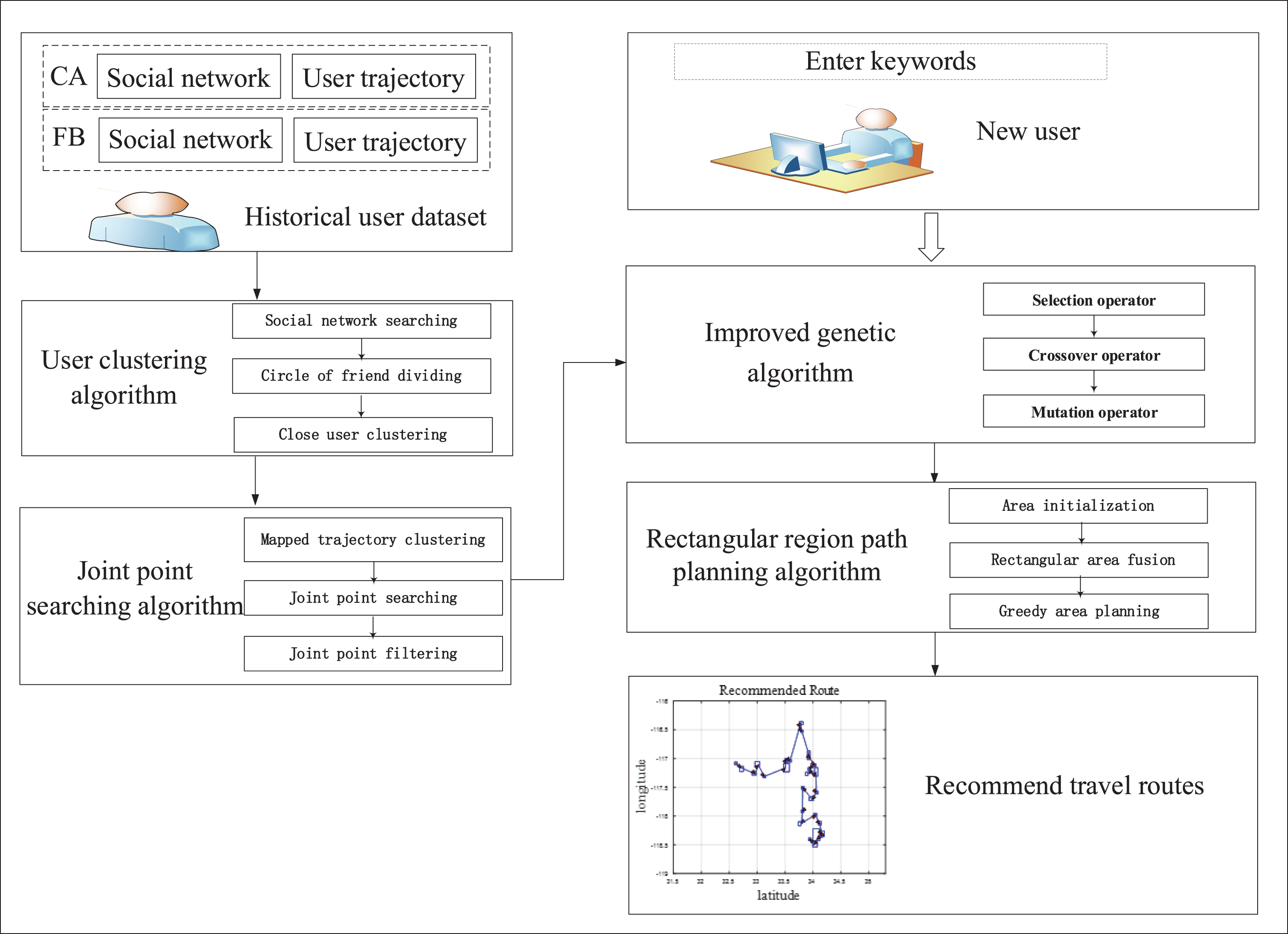
Framework of the proposed route recommendation system.

The contributions of this study are as follows:

For convenience while searching for a path, a user clustering algorithm is proposed to class all historical users according to keywords; the clustering results serve to lock the categories quickly.

An IG algorithm for trajectory recommendation is proposed. The proposed algorithm is used to filter interest points, select the joint points that meet the user’s preferences, narrow the search scope, and make the route recommendation algorithm more efficient.

An efficient route recommendation algorithm based on rectangle area path planning is proposed. The interest points are divided into rectangular areas so that the areas do not overlap with each area has a certain degree of differentiation.

An extensive set of experiments are conducted for performance evaluation and comparison. The Davies–Bouldin index (DBI) and Dunn index (DI) evaluating indicators are used to analyze the clustering results, and the average edit distance and average area coverage are used to measure the final recommendation results.

The organizational structure of this paper is as follows. Section 1 gives an overview of route recommendation methods. Section 2 discusses related studies on tourism route recommendation. Section 3 analyzes user social networks and historical trajectories offline modules, including user clustering algorithms, a hierarchical clustering performance evaluation index, and the joint point search of each clustering result path. Section 4 details the online module recommendation system, including the IG algorithm and path recommendation algorithm. Section 5 verifies the prediction accuracy of the proposed method. Finally, Section 6 summarizes the algorithm and problems solved in this paper and outlines future work.

2 Related work

Presently, the research on tourism route recommendation mainly includes the aspects presented in the following subsections.

2.1 Personalized demand-based methods

Personalized recommendation according to the different travel needs of users is an important task in travel route recommendation. Malik et al. [5] used a neural network and particle swarm optimization to predict the most effective optimal path by considering distance, road congestion, weather, and other factors. Considering optimal path recommendation of a navigation system, Gregor et al. [6] used a neural network to optimize the “soft” attributes (e.g., the level of tourist interest in scenic spots) to determine a path for the highest tourist satisfaction by improve the routing algorithm. For those tourists who only focus on time, Zhu et al. [7] accounted for which month is suitable for travel and which period of the day is suitable for scenic spots, and recommended a tourist route by expanding the longest path generation algorithm. In some special cases, such as limited travel time and bad weather, tourists tend to choose the path with the shortest travel time to the scenic spot. Li et al. [8] optimized the travel time from an online module and offline module to generate a shorter travel time than the existing travel path.

2.2 Real-time demand-based methods

Forecasting the next potential tourist attraction according to current urban traffic, the road network environment, and the real-time needs of tourists is another important task in path recommendation. Zhang et al. [9] used a residual neural network to predict city traffic, while Di et al. [10] and Mehmood et al. [11] utilized the SERM neural network, considering time, distance, attraction, weather, traffic conditions, and other factors to establish a real-time travel route recommendation system, predict the next possible scenic spot for tourists, and recommend a path to tourists for the actual situation. Lin et al. [12] used a hybrid integration algorithm of k-nearest neighbor and Bayesian algorithms to predict information about the next scenic spot.

2.3 Multi-scene demand-based methods

The multi-scenario application of path recommendation is also very extensive. Jesús et al. [13] designed a hiking route for tourism, while Zheng et al. [14], Hong et al. [15], and Gan et al. [16] investigated the trajectory patterns of taxis and ships. In addition, Sun et al. [17] and Gong et al. [18] used a tourist route recommendation method to improve the production efficiency in industrial scenarios.

2.4 Similarity demand-based methods

The similarity of historical trajectories plays an important reference role for route recommendation. In the research on trajectory similarity, clustering algorithms are the most widely used. Han et al. [19] proposed a new trajectory clustering algorithm from the perspective of complete trajectories. Mao et al. [20] proposed an adaptive acid algorithm for trajectory clustering analysis, and Lv et al. [21] conducted trajectory hierarchical clustering from the perspective of personal semantics. Zhang et al. [22] proposed a new hierarchical clustering method using spatio-temporal periodic pattern mining. From the perspective of local semantics, Dong et al. [23] proposed a mining algorithm with a regional semantic trace pattern, which effectively revealed the pattern of local frequent motions.

2.5 Drawbacks of current methods

The aforementioned methods extract trajectory path information from various sources and recommend appropriate routes. However, existing methods fail to achieve a good balance between personalization and diversification. Although Wen et al. [24] proposed a keyword-based framework, which recommends routes from a personalized perspective, the current methods still have low accuracy and lack diversity in their travel route recommendations to users.

Therefore, in this study, we propose an IG method that can achieve personalization while maintaining diversification. The proposed method considers both the attributes of traditional methods and those of path preference. By improving the genetic algorithm to meet the actual scenario, the recommended path is more accurate and diversified.

3 User clustering based on historical trajectory data

To increase personalization in the route recommendation system, this section analyzes the historical trajectory data in advance to ensure that the recommended route reflects the user’s situation. It consists of three parts. First, a clustering algorithm based on the number of friends the users has is proposed. Next, an evaluation standard for the clustering result based on the depth traversal distance tree is proposed. Finally, the experimental results of the proposed method on the Facebook (FB) and Foursquare (CA) datasets [24] are analyzed.

The FB and CA datasets contain two sub-datasets of social networks and user trajectories, respectively. Each data element of the social network sub-datasets includes two data items: user ID and friend ID. The format is u₁, f₁, u₂, f₂, u₃, f₃, u₄, f₄, where u represents users and f represents friends. For example, in 1,2, 3,4, 2,5, 5,6, f₁ and u₃ are the same user, f₃ and u₄ are the same user, user u₁ and f₁ within the same brackets are called direct friends, user u₁ and f₃ are called indirect friends, user u₁ and f₂ are not friends. Next, the social network dataset is used for user clustering.

3.1 User clustering algorithm

To better explain the related algorithms, the following definitions are given.

Definition 1 (Circle of friends): User u and all users who have a direct or indirect relationship with u are called a circle of friends. User u is referred to as the social core.

The circle of friends is a collection of similar users, in which users have direct or indirect contact. Whether online or offline, they will reflect each other’s travel experience. Users with similar hobbies will check the travel of their circle of friends while planning their next trip and the scenic spots to visit.

Definition 2 (Strong connection / Weak connection): For the circles of friends C₁ and C₂ with different social cores, if the number of common friends is greater than the threshold k, then the circles of friends C₁ and C₂ are strong connections. Otherwise, C₁ and C₂ are weak connections.

Different users have different numbers of friends, and users with more friends have stronger social influence than other users. For example, consider users u₁, u₂, and u₃. If u₁ has six friends, u₂ has four friends, and u₁ and u₂ have two good friends in common, then u₁, u₂, and their eight unique friends are clustered into a circle of friends C₁. Assuming that u₃ has 13 friends, and all of them have no direct relationship to u₁ and u₂, u₃ is regarded as part of circle of friends C₂. The social impact between C₁ and C₂ differs. In this section, all users are clustered into several circles of friends according to their friendships. The user clustering pseudocode is shown in Algorithm 1.

Algorithm 1: User clustering.
Input: dataset of multiple trajectories fs_friendship_CA, thresholds k and n
Output: taxonomy result RST
1. Initialize the fs_friendship_CA dataset;
2. RST = {};
3. [long,short] = Segmentation(fs_friendship_CA,n);
4. for each userID_i ∈ long
5. Cof_u_i = userID_is circle of friends;
6. for each friendID_j ∈ Cof_u_i
7. Cof_f_j = friendID_js circle of friends;
8. iffriendID_j exists in short
9. if strong_link(userID_i,friendID_j,k)
10. delete friendID_j from short;
11. Cof_u_i = Cof_u_i⋃Cof_f_j;
12. ifshort is empty exit(0);
13. endif
14. elseif weak_link(userID_i,friendID_j,k)
15. if search_finish(long) exit(0);
16. endif
17. endif
18. endif
19. endfor
20. RST = RST ∪ Cof_u_i;
21. endfor
22. returnRST;

In Algorithm 1, fs_friendship_CA is the input dataset of multiple trajectories. It also takes as inputs the thresholds k and n, and outputs several friend clusters. In Line 3, the Segmentation function sorts all users from high to low according to the number of friends. Then, it selects the top n percent of users as the result of the long matrix according to the threshold value, and the remaining users as the result of the short matrix. Lines 4–8 iterate over all the friend IDs of all the user IDs in the long user matrix. If the friend ID is also used as the user ID in the short matrix, Lines 9–17 judge whether the friend ID and the user ID are strong or weak connections. If they are strong connections, the friend circle of the friend ID is deleted from the short matrix, and if they are weak connections, nothing is deleted. This loop continues until none of the circles of friends have strong connections.

In Algorithm 1, the social core is the center of the circle of friends, and the closely related circle of friends is clustered into several clusters. The users in the cluster generally have similar preferences. At this point, the user’s historical trajectories are not involved. Next, the joint points are searched according to the historical trajectories.

3.2 Joint point search algorithm based on depth-first strategy

This section describes how the keywords in the user’s trajectory map in all the circles of friends are matched according to the keywords entered by the user. If the keyword matching score of circle of friends C₁ is the highest, then the joint point in the trajectory map of C₁ is the result of offline module processing.

Definition 3 (Joint point): In a path-connected digraph with more than three points of interest, if more than two paths pass through the same point of interest (also known as interest point), it is called a joint point.

Table 1 is a user cluster obtained from Algorithm 1, and it contains paths T₁, T₂, and T₃. These three trajectories cross together to form a digraph, as shown in Fig. 2. This section analyzes these directed trajectory diagrams to find the joint points.

Table 1
Example of route dataset

Uid Pid longitude latitude time Tag

T₁ R₁ 40.7314 – 74.0036 7:00 ‘{Shop∖Service}’

T₁ R₂ 40.7314 – 74.0030 9:00 ‘{Office∖Professional∖Other Places}’

T₁ R₃ 40.7171 – 74.0039 10:00 ‘{Travel∖Transport}’

T₁ R₄ 40.7114 – 74.0132 19:00 ‘{Stadium∖Arts∖Entertainment}’

T₁ R₅ 40.7505 – 73.9934 20:12 ‘{Arts∖Entertainment∖Movie Theater}’

T₂ R₆ 40.7559 – 73.9981 3:09 ‘{Travel∖Transport}’

T₂ R₃ 40.7171 – 74.0039 6:33 ‘{Travel∖Transport}’

T₂ R₈ 40.6450 – 73.7845 3:01 ‘{Residence}’

T₂ R₉ 34.0748 – 118.0712 8:26 ‘{College∖University}’

T₃ R₇ 34.1440 – 118.1188 14:32 ‘{Outdoors∖Recreation∖Shop∖Service}’

T₃ R₄ 40.7114 – 74.0132 7:15 ‘{Stadium∖Arts∖Entertainment}’

T₃ R₁₀ 34.1346 – 118.0515 17:32 ‘{Shop∖Service}’

Uid	Pid	longitude	latitude	time	Tag
T₁	R₁	40.7314	– 74.0036	7:00	‘{Shop∖Service}’
T₁	R₂	40.7314	– 74.0030	9:00	‘{Office∖Professional∖Other Places}’
T₁	R₃	40.7171	– 74.0039	10:00	‘{Travel∖Transport}’
T₁	R₄	40.7114	– 74.0132	19:00	‘{Stadium∖Arts∖Entertainment}’
T₁	R₅	40.7505	– 73.9934	20:12	‘{Arts∖Entertainment∖Movie Theater}’
T₂	R₆	40.7559	– 73.9981	3:09	‘{Travel∖Transport}’
T₂	R₃	40.7171	– 74.0039	6:33	‘{Travel∖Transport}’
T₂	R₈	40.6450	– 73.7845	3:01	‘{Residence}’
T₂	R₉	34.0748	– 118.0712	8:26	‘{College∖University}’
T₃	R₇	34.1440	– 118.1188	14:32	‘{Outdoors∖Recreation∖Shop∖Service}’
T₃	R₄	40.7114	– 74.0132	7:15	‘{Stadium∖Arts∖Entertainment}’
T₃	R₁₀	34.1346	– 118.0515	17:32	‘{Shop∖Service}’

Fig. 2

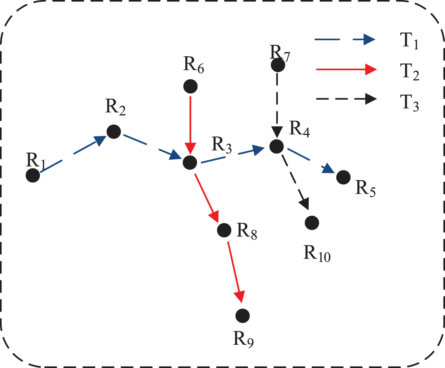
Trajectory of a friendship cluster.

In this study, the traditional depth-first search (DFS) algorithm is improved. Algorithm 2 determines in advance whether the user’s trajectory graph can search for the appropriate joint points. If the user’s trajectory graph is not a connected graph, no joint points can be found. Otherwise, the proposed ImpDFS function will be called.

The ImpDFS function searches for joint points in the connected graph. The joint point searching pseudocode is shown in Algorithm 2.

The input of Algorithm 2 is the path digraph obtained by Algorithm 1. If the digraph is unconnected or doubly connected, all the resulting matrices returned are – 1. If the digraph is simply connected, the joint points of the graph are searched.

Algorithm 2: Joint point searching.
Input:digraph of all users’ trajectories All_G = (V, E), RST
Output:dataset of joint points A
1. Convert trajectories related to users in RST into digraph G = (V’, E’);
2. Initialize A = -1;
3. ifG is a path-connected digraph
4. Select the head node s as the starting vertex;
5. A = ImpDFS(s, 0);
6. endif
7. return A;
Function 1: A = ImpDFS(Node v, int predfn)
1. Mark(v, visited); predfn = predfn +1;
2. artpoint = false; count = 0;
3. A = B[v.id] = predfn;
4. for each (v,w)∈E
5. if (v,w) is a tree edge or a forward edge
6. ImpDFS(w, predfn);
7. B[v.id] = minB[v.id], B[w.id];
8. if B[w.id] > = A[v.id]
9. artpoint = true;
10. endif
11. elseif (v,w) is a back edge
12. B[v.id] = minB[v.id], A[w.id];
13. endif
14. endfor
15. ifartpoint = = true
16. count = count +1;
17. A[count] = v;
18. endif
19. return A;

In Function 1 (ImpDFS), v and w are nodes, predfn is the depth of the node, and v.id represents the user ID of node v. Lines 2–3 initialize the variables artpoint, count, A[v.id], and B[v.id], where artpoint is used to determine whether the node is a joint point; count is used to count the number of joint points, and A[v.id] and B[v.id] are the record variables of the node. In Lines 4–14 of the ImpDFS function, the depth traversal trace graph is used to determine each variable in the graph G. If B[w.id] is greater than or equal to A[v.id], where w is a child node of v, then it can be determined whether or not v node is a joint point (i.e., the artpoint of node v is set to true). Finally, in Lines 15–19, A[count] stores node v and returns the corresponding result.

The joint points obtained by Algorithm 2 are overlapping interest points in a circle of friends. That is, within a circle of friends, different users appear at the same location, and these particular interest points attract the users. As shown in Fig. 3, the joint points reflect the most interesting places among numerous optional interest points, and are the most visited scenic spots for tourists. The travel route will be recommended according to the joint point below.

Fig. 3

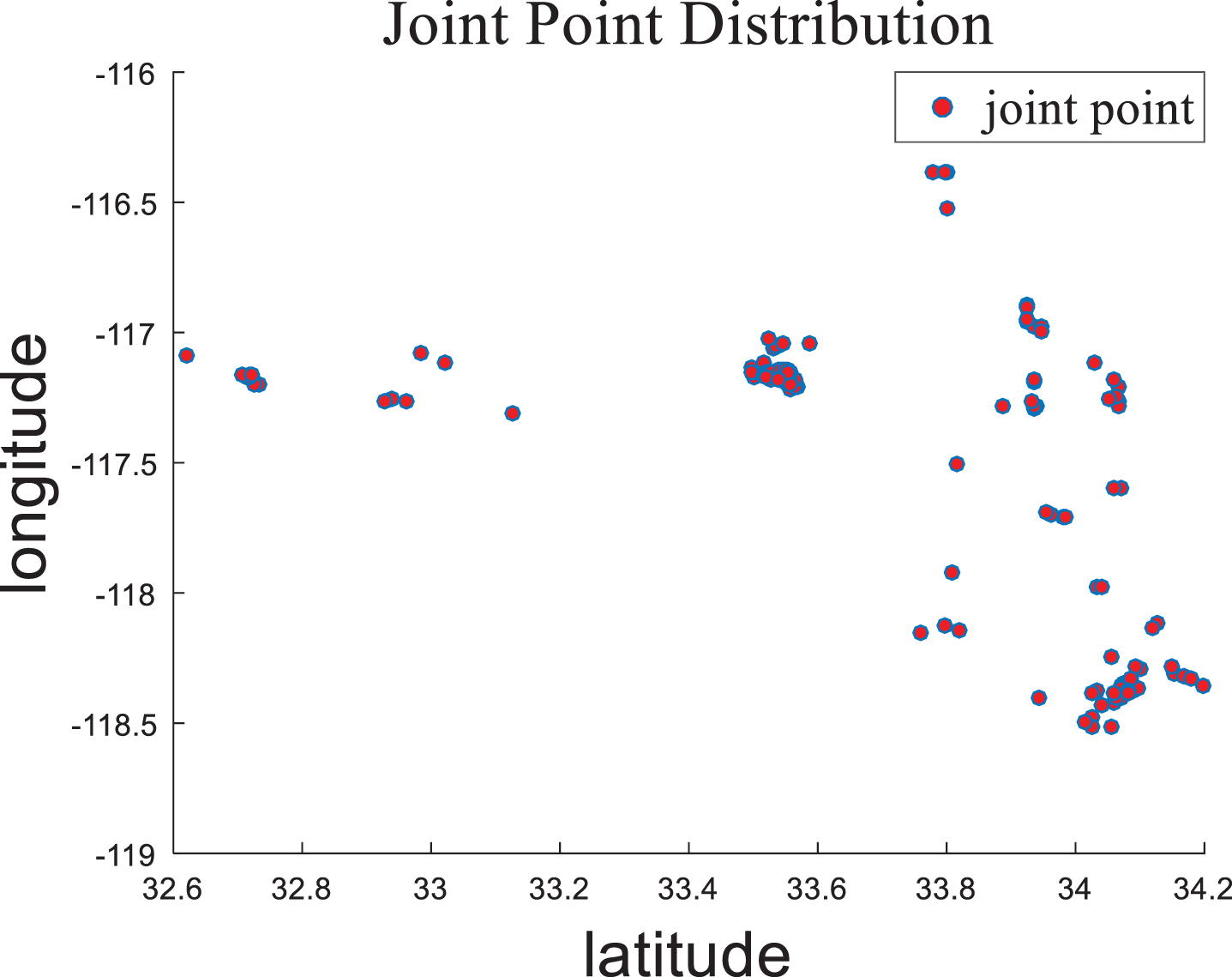
Example of joint point distribution.

4 Improved genetic algorithm for trajectory recommendation based on keyword search

The joint points obtained by Algorithm 2 contain the keywords describing the scenic spots. In this section, the keywords entered by the user are used to filter these interest points again, select the joint points that meet the user’s preferences, narrow the search scope, and make the route recommendation algorithm more efficient. Then, the IG algorithm is used to pre-recommend the routes that satisfy the factors of the user’s time, distance, and desired attraction. Finally, the shortest path method for rectangular regions is used to recommend a tourist route to users.

4.1 Joint point filtering

To filter out the joint points that meet the user’s requirements in the results of Algorithm 2, this study proposes a method to measure the correlation between the user’s requirements and the joint points. This is represented by $Relevance = max_{l \in S} \frac{(\sum_{w \in K} f (w))^{2}}{| | C_{l} | |},$ (1) where w refers to a keyword entered by the user, f(w) refers to the number of keywords w contained in the C_l cluster, and ||C_l|| refers to the number of all keywords in the C_l cluster. Equation can measure the correlation between user input keywords and path interest point keywords. Each user cluster C will have a relationship value. The interest point that has the largest relationship value is selected, which coincides with the joint point in Algorithm 2 as the selected joint point.

Figure 4 shows the matching friend clusters when K = {“doors,” “travel,” “shop”} and the actual image of the user’s trajectory.

Fig. 4

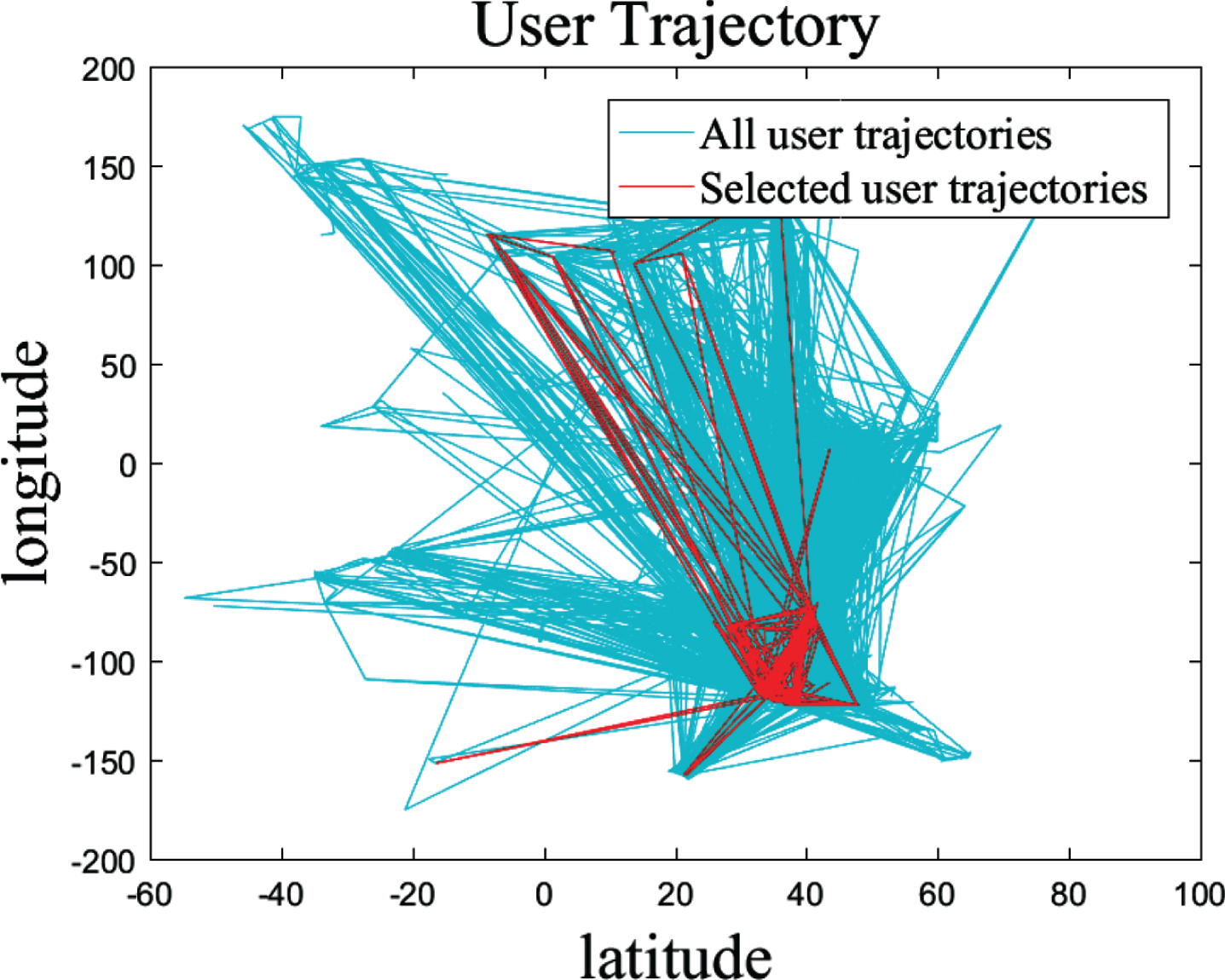
User actual trajectory in a cluster.

The blue area is the trajectory image of all users, involving multiple regions around the world. The red path is the path obtained by friend clustering. This subsection described how the joints to be recommended from the joints in the red area are selected, and the next subsection describes how the recommended route based on these joints is generated.

4.2 Improved genetic algorithm idea

The advantages of genetic algorithm are that it can handle conditional constraints well, has strong global search ability, and can avoid local optimal solutions while obtaining the global optimal result. The objective of this study is to recommend a global optimal route to the user; hence the genetic algorithm algorithm is the most suitable scheme. In this subsection, the genetic algorithm [25 –27] is improved to organize the selected joint points in the previous subsection. First, the interest points on the historical user access path are associated with individuals. Then, the fitness function is determined according to the actual situation, and the appropriate selection operator, crossover operator, and mutation operator are generated. Finally, the recommended tourist path in the region is obtained from the global convergence to a local region. Concurrently, the algorithm can change the search range of the path, run using different granularities, and obtain flexible personalized recommendation results. All points of interest are encoded by floating-point coding, such as 1,2 ... n. Some of the n points are selected for iterative calculation.

4.2.1 Fitness function

This study determines the fitness function via three components: (1) relevance of the user’s input keywords for the individual, (2) Euclidean distance of the pre-recommended path, and (3) access time of the pre-recommended path.

The user relevance factor considers the relationship between the route label and the keyword entered by the user. If the label on the route is similar to the keyword entered by the user, the route is considered to meet the personalized needs of the user. The fitness formula is $RV \propto \frac{(\sum_{w \in K} f (w))^{2}}{∥ T_{i} ∥},$ (2) where ∑_w∈Kf (w) refers to the number of times all keywords in the keyword set K appears in the path and ||T_i|| refers to the number of keywords in all tags in the path.

The distance factor considers the relationship between the pre-recommended route and the user’s preference. If the distance of the individual decoding route is short, the route is considered to meet the actual needs of the user. The distance factor formula is $PV \propto \frac{1}{{dtc}_{{Tra}_{i}}},$ (3) where dtc_{Tra
_i} refers to the actual distance of the individual path Tra_i. Considering the influence of the time factor on this route, it is assumed that the appropriate tour time of each interest point is a fixed time in the day and that the tour time of historical users conforms to that time pattern. The sequence obtained after the gene coding is reversed is called the reverse sequence. If the number of reverse sequences in the path time series is large, the path is considered to deviate from the actual needs of users. Otherwise, it is considered to meet the needs of users. The formula for the time factor is $TV \propto \frac{∥ {Tra}_{i} ∥}{RO},$ (4) where RO is the number of time inverses after decoding the Tra_i path.

Combining the above three factors, the fitness function is as follows: $Fit = α \times RV + β \times PV + γ \times TV,$ (5) where α, β, and γ are, respectively, the weights for the three factors; the sum of the three weights is “1.”

4.2.2 Selection operator

A random competitive selection method is used as the selection operator. Two individuals are selected according to the roulette algorithm each time, and then the two individuals compete to select the individuals with high fitness as the cross mutation operation. The probability that an individual is selected is directly proportional to the fitness function. If the size of the population is n and the fitness of the individual is Fit_i, then the probability of its selection is $p_{i} = {Fit}_{i} / \sum_{j = 1}^{n} {Fit}_{j}$ .

4.2.3 Crossover operator

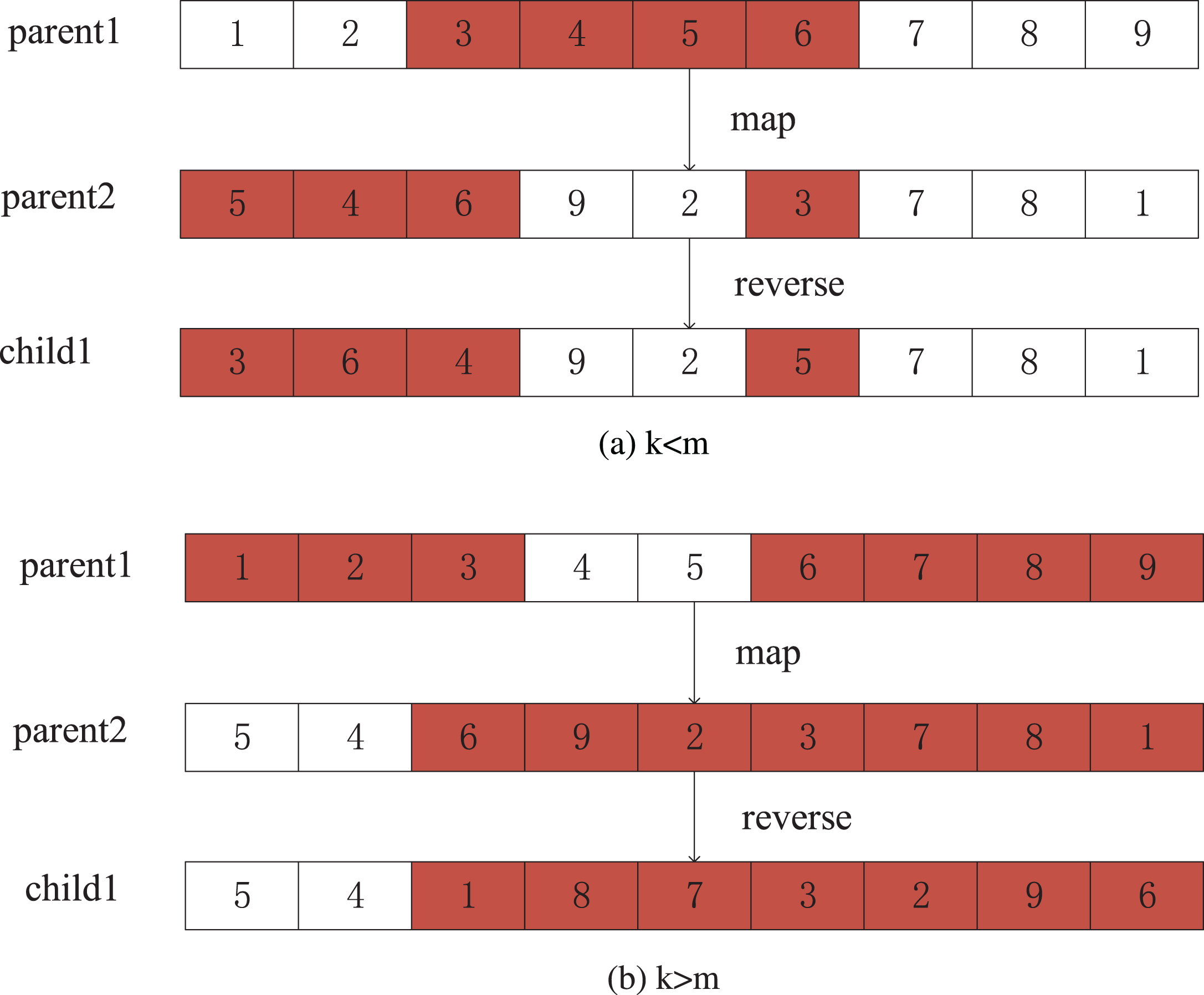
This study proposes a novel crossover operator, which can make individual variations meet the requirements of efficiency and high speed. For example, there are two individuals of length n, parent1: 123456789 and parent2: 546923781. First, two unequal numbers between one and n are randomly generated. If the random numbers are, for example, k = 3 and m = 6 (k < m), Fig. 5(a) is used. The gene with a parent1 index that is greater than or equal to k and less than or equal to m is removed, and it is then mapped to the index of parent2. Then the gene in parent2 is reversed to obtain the gene 364925781. Finally, the positions of parent1 and parent2 are interchanged again, and offspring 2196453782 is obtained.

Fig. 5

Crossover operator.

In contrast, if k = 6 and m = 3 (i.e., k > m), as shown in Fig. 5(b), then all the indices of gene subscripts of parent1 smaller than m and larger than k are removed. Then the genes are mapped to parent2, and these genes are reversed on parent2 to obtain children1: 541873296. In summary, by changing the positions of parent2 and children1, children2: 827654319 is produced.

4.2.4 Mutation operator

The path analysis reveals that the interest points are not evenly distributed. Some points are densely distributed, and others are sparsely distributed. That is, not all the interest points are concentrated in a high-density region, and there are always several interest points far away from the center of the high-density region. The user will generally give up these points; hence, they can be deleted. In this section, the mutation operator is used to delete those points where the possibility of user access is below the threshold.

An interest point in the path is randomly selected assuming that the path length changes less than the distance threshold e after deleting the interest point. The similarity of the interest point to the center of the recommended path is determined, and the interest point is retained. If the threshold is greater than e, the point is redundant, and the interest point is deleted. The number of genes in the population remains stable.

4.3 Improved genetic algorithm

The pseudocode of the proposed IG algorithm is presented in Algorithm 3.

Algorithm 3: Improved genetic algorithm.
Input: set of keywords input by the user K, digraph of all users’ trajectories All_G = (V, E), RST
Output: recommended population RP
1. Initial trajectory path;
2. Select the circle of friends with the highest relevance using Equation (1);
3. Find all joint points of this circle of friends;
4. Encode joint points as genes;
5. Initialize population according to the genes;
6. Sort population in descending order according to the fitness values of genes calculated by Equation (5);
7. RP = {};
8. repeat:
9. for each gene g in population
10. Selection_operator(g);
11. Crossover_operator(g);
12. Mutation_operator(g);
13. Replace the gene with the smallest Fit value
with the new gene and resort the population;
14. endfor
15. RP = RP∪population;
16. until the population no longer changes;
17. returnRP;

In Line 1, the trajectory path is initialized, all the trajectory paths are processed uniformly, and a number is assigned for each longitude and latitude value. In Line 2, the degree of association between each circle of friends and the keyword set K input by the user is calculated via Equation (1), and a relation circle of friends about several users is obtained. In Line 3, the joint points in this circle of friends are found. Line 4 encodes the joint points as several strings. In Line 5, these genes are randomly duplicated to form a population. Line 6 uses Equation (5) to calculate the fitness of each genetic individual. The adaptability is arranged from high to low to obtain a standardized group. Line 7 initializes the recommended population. Lines 8–16 iterate over the individuals in the group and select, cross, and mutate the individuals. Then it chooses two individuals to replace the individuals with low Fit values in the group, iterates several times, and obtains the individuals with the highest Fit values. The experimental results of Algorithm 3 are shown in Fig. 6.

Fig. 6

Trajectory image with different iterations of the improved genetic algorithm.

The three distance parameters used in the mutation process of the IG algorithm are 0.001, 0.01, and 0.1, respectively. When the distance parameter is 0.001, the interest points recommended by the genetic algorithm are concentrated at one point, which is not suitable for medium and long distance travel recommendation. If the distance parameter is 0.01, Fig. 6(a), (c), and (e) are obtained. The trajectory image tends to converge in a block. If the distance parameter is 0.1, Fig. 6(b), (d), and (f) can be obtained. The interest points can be located in a large area, and the corresponding recommended interest points can be relatively sparse.

In this study, different distance parameters are used. If the user needs to locate a point that is most suitable for personal interest, the distance parameter can be 0.001, and the system will return a point of interest. If the user wants to travel in the short and medium term, the distance parameter can be set to 0.01, and the system will return the area that is most suitable for the user’s needs and more points of interest will be returned for the user to visit. If the user plans to travel for a long time, the distance parameter can be set to 0.1, and the system will return the interest points that meet the user’s personal preferences in a large area. The following path recommendation algorithm uses short and medium-term travel by default, and the distance parameter is set to 0.01.

4.4 Route recommendation

Using the genetic algorithm to obtain several historical trajectory points that satisfy the user’s input keywords, users in the region can reach places by using vehicles, ships, and other medium and low-speed vehicles. According to the analysis of these trajectories, there are numerous interest points generated by the different keywords entered by users. According to the average walking speed of human beings, a rectangular moving range can be defined, within which users can walk to the point of interest.

The interest points are divided into rectangular regions so that all regions do not overlap and have a certain degree of differentiation. Route planning is then carried out between regions. Algorithm 4 is listed below.

Algorithm 4: Rectangular region path planning algorithm
Input: recommended population RP, set of keywords input by the user K
Output: shortest path Γ
1. Convert trajectories related to RP into digraph G’;
2. m = 0;
3. for each path_i in G’
4. for each point_j in path_i
5. Expand a rectangle centered on point_j;
6. if there are rectangles with intersections
7. Merge these intersecting rectangles to expand the rectangle and delete the new points within the merged rectangle;
8. m = m +1;
9. endif
10. endfor
11. endfor
12. Find the point that best satisfies user’s requirement as a starting point and push it into the path priority queue Γ;
13. fori = 1:m
14. Find the rectangular point closest to the tail point of the path priority queue Γ;
15. Put this point at the end of the path priority queue Γ;
16. endfor
17. returnΓ;

Line 1 initializes the input data. If different users visit the same place, delete it and renumber the interest points. In Line 2, the variable m refers to the number of matrix region fusions. Lines 3–4 search every point in G’. In Line 5, the minimum matrix block is established with the point of interest as the center. Lines 6–9 expand the matrix range in turn, with each minimum matrix block as the center, where Line 7 merge partially coincident rectangles. Line 12 looks for the most suitable interest point and sends it into the path priority queue. Lines 13–16 use the greedy method to plan the path between points in the matrix blocks. Line 17 returns the path the user needs.

Algorithm 4 recommends the last step based on the pre-recommended route. First, each point of interest in the pre-recommended route is used as the initial rectangular region, and then extended in the final rectangular region. Taking the rectangular area as the recommended scenic spot, the shortest route is recommended. The experimental results of Algorithm 4 are as shown in Fig. 7. The recommended route in this study starts from the matrix area that best meets the user’s requirements. This area contains interest points and is the area that users can walk to within a certain amount of time. The greedy algorithm is then used to select the next matrix region. On the recommended route, users can visit all interest points that meet their personal preferences in the most efficient timeframe.

Fig. 7

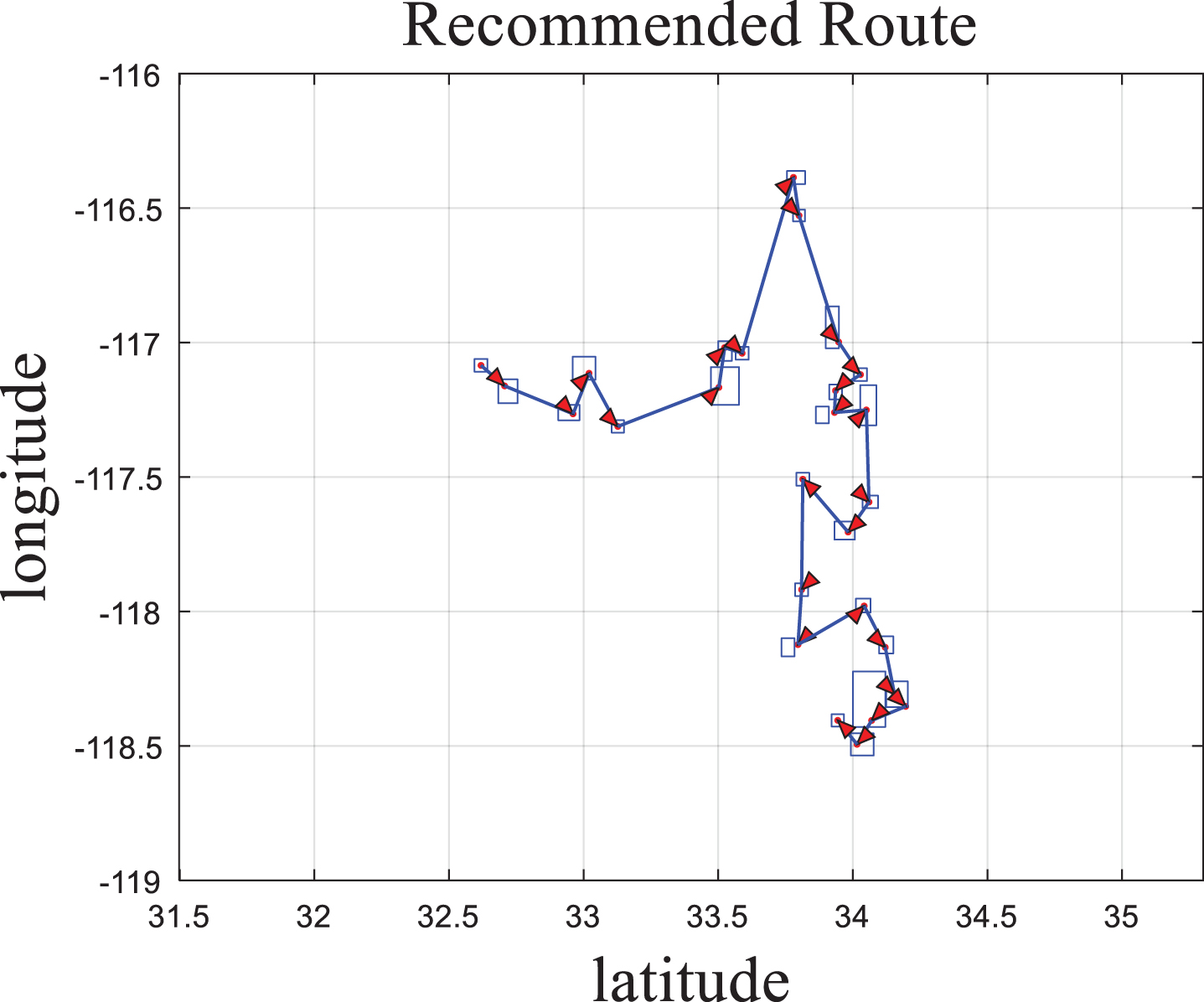
Example of recommended route.

5 Experimental evaluation

Location-based social networking (LBSN) is a new service that combines time series, behavior trajectories, and geographic location information. This study uses two offline LBSN datasets, as shown in Table 2. The FB dataset contains valid data collected from Facebook, including user social relationships and trajectories. The CA dataset is a dataset of social relationships and trajectories of 96 users and their friends in the Taiwan Province of China. Both datasets are from the literature [24].

Table 2
Details of the LBSN datasets

Property Network

FB CA

Check-in 869,317 483,813

User 29,512 4,136

Friend 39,513 32,512

POI 225,077 121,142

Property	Network
Check-in	869,317	483,813
User	29,512	4,136
Friend	39,513	32,512
POI	225,077	121,142

5.1 Experimental platform and dataset

The computing equipment used for the experiment included a 3.2 GHz 4 Core (TM) i5-8400 CPU, 16 GB memory, and 64 bit Windows 10 OS. The proposed algorithms were realized in MATLAB 2016a.

The FB and CA datasets have two sub-datasets, respectively. The first sub-dataset is the user’s social network data. The FB dataset has 29,512 users and 39,513 friends of users. The CA dataset has 4,136 users and 32,512 friends of users. The second sub dataset is the trajectory data of all users, including the longitudes and latitudes of the tour sites, times, and keyword descriptions of the points of interest.

5.2 Clustering results of evaluation on Algorithm 1

The clustering algorithm proposed in Section 3 uses the first subset of the FB and CA datasets. The result of clustering requires a criterion to determine its advantages and disadvantages. For the evaluation of clustering results, two types of evaluation indices are generally used. One is the external index, which is used to compare the clustering results to a “reference model.” The other is the internal index, which is used to investigate directly the clustering results without using any other reference model [28]. In this paper, the original social relations are clustered into several clusters, which need to satisfy the requirements of low similarity between clusters and high similarity within clusters. Because there is no reference model for the clustering results in this study, internal indicators are used to evaluate directly the clustering results. The cluster division in the clustering results is accounted for by $avg (C) = \frac{2}{| C | (| C | - 1)} \sum_{1 ⩽ i < j ⩽ | C |} dist (\vec{x_{i}}, \vec{x_{j}}),$ (6) $diam (C) = max_{1 ⩽ i < j ⩽ | C |} dist (\vec{x_{i}}, \vec{x_{j}}),$ (7) $d_{min} (C_{i}, C_{j}) = min_{\vec{x_{i}} \in C_{i}, \vec{x_{j}} \in C_{j}} dist (\vec{x_{i}}, \vec{x_{j}}),$ (8) $d_{cen} (C_{i}, C_{j}) = dist (\vec{u_{i}}, \vec{u_{j}}),$ (9) where the dist() function in Equations (6)–(9) is used to calculate the distance between two sample vectors $\vec{x_{i}}$ and $\vec{x_{j}}$ , avg(C) in Equation (6) is the average distance between samples in set C, diam(C) in Equation (7) is the longest distance between samples in set C, d_min(C_i, C_j) in Equation (8) corresponds to the distance between the closest samples in set C_i and set C_j, d_cen(C_i, C_j) in Equation (9) corresponds to the distance between cluster C_i and cluster C_j, and the vector in Equation (9) represents the center point of set C: $\vec{u} = \frac{1}{| C |} \sum_{1 ⩽ i < j ⩽ | C |} \vec{x_{i}}$ .

The DBI, which represents the similarity between different sets, is given by $DBI = \frac{1}{k} \sum_{i = 1}^{k} max_{j \neq i} (\frac{avg (C_{i}) + avg (C_{j})}{d_{cen} (u_{i}, u_{j})}) .$ (10)

The smaller the DBI value is, the better. In addition, the DI [28], which represents the similarity between each element in the set, is given by $DI = min_{1 ⩽ i ⩽ k} {min_{j \neq i} (\frac{d_{min} (C_{i}, C_{j})}{{max}_{1 ⩽ l ⩽ k} diam (C_{l})})} . .$ (11)

The larger the DI value, the better.

Because the social relationship of user input in Algorithm 1 does not have a distance, this study proposes a sample distance inference method to evaluate the performance of Algorithm 1. This is done by constructing a distance tree for all users’ social relations. The sample distance is related to the level of the tree. The definition of distance tree is as follows.

Definition 4 (Distance tree): Assume an n-branch tree with an empty node as the root node. Select a sub-node and recursively form another sub-node tree with this sub-node as the root node until the distance tree contains all the user nodes.

According to Definition 4, the root node should be selected to make the n-tree as similar to the user’s social relationships as possible. Thus, the sub-node with the largest number of friends should be selected to make the distance representing the user’s social relationships more accurate. This node is called the initial node. The data structure of each node in the designed distance tree is shown in Table 3.

Table 3

Node data structure

Node data	Hierarchy	Parent node	Child node	Tag
data1	3	data2	data3	false

Node data refers to the index of the user’s personal information, which points to the user’s personal trajectory information. Hierarchy refers to the number of layers of this node’s data in the n-tree, which indicates that this node is closely related to the user’s social contact in the previous layer. The core user point is the circle of friends of the parent node. The child node refers to other user indices of the core user point. The tag is used to record whether or not the node has been accessed (false means it has not, and true means it has).

The process of constructing the social relationship distance tree of users is shown in Algorithm 5.

Algorithm 5: Construct distance tree.
Input: RST
Output: distance_tree
1. Initialize RST, distance_tree;
2. pdata = search_origin_data(RST);
3. repeat:
4. ifpdata.tag = = true
5. Insert pdata into distance_tree;
6. Construct_tree(pdata.childnode);
7. else
8. pdata.parentnode = search_parent_data(pdata,RST);
9. pdata.hierarchy = pdata.parentnode.hierarchy +1;
10. pdata.childnode = search_child_data(pdata,RST);
11. pdata.tag = true;
12. Construct_tree(search_brother(pdata, RST));
13. endif
14. until all the pdata.tags in RST are true;
15. returndistance_tree;

Line 1 of Algorithm 5 initializes RST as the input. Line 2 finds the initial node in the input data. If the fourth line determines that the node has been visited, the fifth line is processed, and the child nodes of the processing node are traversed. If it is determined that the node has not been accessed, the node data will be processed in Lines 8–11. In Line 8, the function search_parent_data is the parent node found in RST. In Line 9, the level of the node is declared. In Line 10, the function search_child_data is the child node found in RST. In Line 11, the node pdata will be labeled as accessed. In Line 12, the function search_brother finds the next sibling node of the node pdata, and then traverses the sibling node. Line 14 is the stop condition of the algorithm (i.e., it stops when all the input data RST have been accessed). Line 15 returns the generated distance tree. In Algorithm 1, different k values are input to generate different clustering results. In the offline module, the optimal clustering results are required. The appropriate k value is used to ensure that the similarity between each circle of friends is the lowest and the difference is the highest.

Algorithm 6 is used to analyze two parameters n and k. The first parameter, n, is the percentage of the segmentation function parameter in Algorithm 1 required to segment the circle length. The second parameter is the threshold k, which determines the strength of the connection.

Algorithm 6: Calculate DBI and DI values.
Input:fs_friendship_CA, thresholds n and k
Output:DBI and DI
1. Initialize ns = [25, 50, 75];
2. Initialize ks = [2,3,4,5,6,7,8,9,10];
3. distance_tree = Construct_tree(fs_friendship_CA);
4. fork in ks
5. forn in ns
6. result = User_Clustering(fs_friendship_CA, k, n);
7. Calculate_DBI_DI(result, distance_tree);
8. endfor
9. endfor
10. returnDBI, DI;

In Lines 1–2, the initial n values are 25, 50, and 75, and the initial k values are the integers from 2 to 10. The value of k is temporarily assigned to one of the nine integers from 2 to 10 (k = 1 is not considered here; k = 1 combines all users as a whole). In Line 3, Algorithm 5 is called to generate the distance tree, where the input data are the user’s social relationship data. In Lines 4–9, different k and n values are entered periodically. Line 6 calls Algorithm 1 in Section 3.1. Line 7 calculates the DBI and DI values according to Equations (10) and (11), respectively.

The experimental results of Algorithm 6 are shown in Fig. 8.

Fig. 8

DBI and DI values for different k values of FB and CA datasets.

According to Fig. 8(a) and (c), when k = 2, the DBI is at its maximum value, and then decreases with increasing k. When n = 25, the DBI is greater than when n = 50 and n = 75. According to Fig. 8(b) and (d), for the same k value, when n = 25 and n = 50, the minimum DI value is obtained. When k is between 2 and 5, the DI value for n = 25 is significantly less than the DI value for n = 50. To sum up, when n = 25 and k = 2, it can meet the evaluation requirements of a large difference between clusters and achieve better clustering results.

5.3 Comparison of route recommendation models

The method proposed in this study is now compared to the following five path recommendation models.

Pattern aware trajectory search (PATS) [29]. The PATS model mainly considers the sum of the scores of all points of interest on the recommended route. Then it scores each pre-recommended route. The route with the highest score is the recommended route of the PATS model.

Time-sensitive routes (TSR) [30]. The TSR model mainly considers the score of the travel route time factor and calculates the total score of each pre-recommended route. The route with the highest score is the route recommended by the TSR model.

Geo-social influenced routes (GSI) [31]. The GSI model considers the social factors and calculates the total score of each pre-recommended route. The highest-scoring route is the recommended route of the GSI model.

Keyword-aware skyline travel route (KSTR) [30]. The KSTR method integrates the user’s geographic movements, time, and social network features into the recommended route in the probability score model.

Keyword-aware representative travel route (KRTR) [24]. The KRTR method uses the representative skyline concept to weigh the geography, attributes, and time characteristics of points of interest. It can recommend the route that best meets the user’s personal requirements in a short time.

Compared with aforementioned five algorithms, the proposed method is more comprehensive in attribute, as shown in Table 4.

Table 4
Attribute comparison of different methods

Algorithm Point of interest Time Social relationship Dynamic geographic information Static geographic information Path preference

PATS ✓

TSR ✓ ✓

GSI ✓ ✓ ✓

KSTR ✓ ✓ ✓ ✓

KRTR ✓ ✓ ✓ ✓ ✓

IG ✓ ✓ ✓ ✓ ✓ ✓

Algorithm	Point of interest	Time	Social relationship	Dynamic geographic information	Static geographic information	Path preference
PATS	✓
TSR	✓	✓
GSI	✓	✓	✓
KSTR	✓	✓	✓	✓
KRTR	✓	✓	✓	✓	✓
IG	✓	✓	✓	✓	✓	✓

This paper evaluates the experimental results using three different aspects: user edit distance, area coverage [24], and algorithm time complexity.

Definition 5 (Edit distance): Edit distance refers to the minimum number of operations in the sequence of interest points of two paths. The allowed operations include inserting interest points, deleting interest points, and replacing interest points.

Definition 6 (Area coverage): Area coverage (also known as coverage ratio) refers to the ratio of the rectangular area of the test path to the rectangular area of the recommended path.

5.3.1 Edit distance comparison

The calculation results of the edit distance are shown in Fig. 9(a) and (b).

Fig. 9

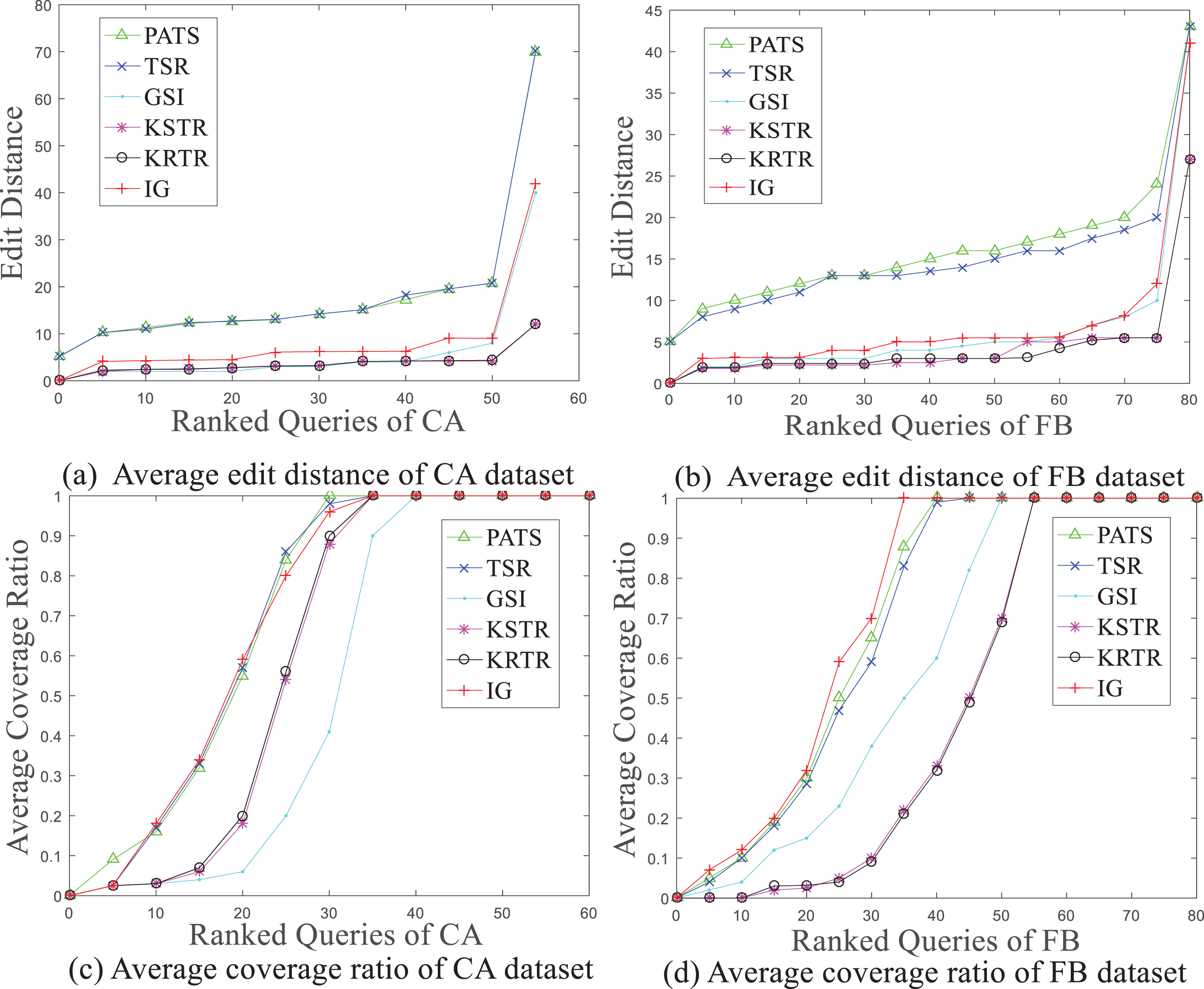
Average edit distance and average coverage ratio versus the recommended travel routes of the CA and FB datasets.

The results of Fig. 9 show that the edit distance of the IG method is greater than that of the GSI, KSTR, and KRTR methods, but less than that of the PATS and TSR methods. In the GSI, KRTR, and KSTR methods, the recommended route is to reconstruct a small number of user trajectory data such that there are more parts overlapped with the sequence of interest points in the test data. However, the PATS and TSR methods only consider the point of interest, and do not consider the user’s entire trajectory. Thus, there is less overlap with the test data. The IG method proposed in this study considers multiple user trajectories. Therefore, its edit distance is larger than that of the GSI, KRTR, and KSTR methods, but smaller than that of the PATS and TSR methods. The statistical results are as shown in Table 5; the average area coverage rate of the proposed method is better than that of the other algorithm, with increasement ratios of 1.04%, 1.96%, 21.39%, 23.68%, and 31.80%, respectively.

Table 5

Comparison of average edit distance and average coverage ratio

Algorithm	Average edit distance of CA dataset	Average edit distance of FB dataset	Average edit distance	Average coverage ratio of CA dataset	Average coverage ratio of FB dataset	Average coverage ratio
PATS	18.4733	16.1765	17.3249	0.6892	0.6865	0.6879
TSR	18.5450	15.0294	16.7872	0.6873	0.6756	0.6815
GSI	6.3333	6.4706	12.8039	0.5127	0.5800	0.5464
KSTR	3.7342	4.5235	4.1289	0.5935	0.4674	0.5305
KRTR	3.7717	4.4647	4.1177	0.5988	0.4648	0.5274
IG	8.5208	7.0941	7.8075	0.6842	0.7059	0.6951

5.3.2 Regional coverage comparison

For the FB and CA datasets, the area coverage of the IG method is compared to the above five methods. As shown in Fig. 9(b) and (d), in the CA dataset, the area coverage of the IG method is better than the above five methods combined. Considering the average area coverage, the IG method selects the appropriate interest points from the global trajectory data for path planning. In terms of the global interest points and the user trajectory that meets the requirements, it performs better than the KRTR, KSTR, and GSI methods. In terms of regional coverage, it performs better than the PATS and TSR methods.

5.4 Time complexity analysis

Suppose that the number of users in the offline dataset is n, the number of interest points is m, and the average length of each user’s historical trajectories is L. The algorithm of the IG framework in this study mainly consists of four steps: (1) analyze the social relationship of historical users in advance; (2) calculate the joint points in the user group; (3) improve the genetic algorithm to select the region; (4) segment the region and recommend the route. The algorithm of constructing a distance tree by a depth-first traversal and calculating DBI and DI values are not the main time-consuming factors in the path recommendation system, and are therefore ignored in this study.

The social relationships of users are analyzed in advance, and the users with close relationships are grouped into a cluster. The time taken by the segmentation function to divide the number of friends is O(L), and the time taken to traverse the social network of users is O(n²). Thus, the time used in this first part is O(L + n²). The traversal of each user’s interest point in depth takes the most amount of time in the calculation of the joint points in the user group. Therefore, the time of O(n²) is used. In the IG algorithm, the initialization time is a constant, O(1), which can be ignored. The main time-consuming step is the calculation of genetic operators, and that takes O(n²). In the fourth part, the time taken to segment the area and recommend the route is O(m²). In conclusion, the calculation timeframe of the IG algorithm is O(L + c₁n² + c₂n² + c₃n² + c₄m²), where c_i is a constant parameter. The value of m is much greater than that of L and n, so the algorithm complexity of the IG method is O(m²).

6 Conclusion

This study focused on the issue of travel route recommendation. The current recommendation model lacks personalization and diversity. This study developed an IG algorithm that mainly considers the influence of friends, the appropriate travel time in the path, and the possibility of meeting the user’s expectations. In the IG model, a series of keywords are first used to describe the path required by users, and the historical data of similar users are analyzed. The proposed method repeatedly screens out the joints that meet user requirements, and uses an IG algorithm to select the appropriate joints from the global region. Then these joint points are divided into matrix blocks, and route planning is carried out between them.

The experimental results showed that the average area coverage is superior to that of the traditional methods. The IG algorithm proposed in this study can be used in social services based on mobile location to provide users with personalized and satisfactory travel route recommendation services. The IG algorithm is suitable for medium and long distance travel, but not for short distance travel, because it is difficult to extract attributes of short-distance travel, which leads to large deviations. In future work, we will improve the diversity of user input and the implementation efficiency of the framework to achieve more accurate recommendations of user paths. Learning from the research method presented in [32], analyzing the movement law of popular routes in scenic spots in recent years and subsequently predicting future travel trends is also a topic worthy of research.

Footnotes

Acknowledgments

The authors would like to thank the reviewers for their useful comments and suggestions for this paper. This work was supported by the National Natural Science Foundation of China (Grant Nos. 61702010, 61972439, 61672039).

References

Zheng

, Trajectory Data Mining: An Overview, ACM Trans Intell Syst Technol 6(3) (2015), 1–41.

Adnan

, Gazder

and Yasar

A.H.

, Estimation of travel time distributions for urban roads using GPS trajectories of vehicles: a case of Athens, Greece, Personal and Ubiquitous Computing (2020), 1–10.

Yin

, Wu

and Sun

, Optimizing last trains timetable in the urban rail network: social welfare and synchronization, Transportmetrica B 7(1) (2019), 473–497.

Chen

, Wu

and Li

, Green Vehicle Routing and Scheduling Optimization of Ship Steel Distribution Center Based on Improved Intelligent Water Drop Algorithms, Mathematical Problems in Engineering 9 (2020), 1–13.

Malik

and Kim

D.H.

, Optimal travel route recommendation mechanism based on neural networks and particle swarm optimization for efficient tourism using tourist vehicular data, Sustainability 11(12) (2019), 3357–3383.

Jossé

, Schmid

K.A.

and Züfle

, Knowledge extraction from crowdsourced data for the enrichment of road networks, GeoInformatica 21(4) (2017), 763–795.

Zhu

, Hao

and Chi

, FineRoute: Personalized and Time-Aware Route Recommendation Based on Check-Ins, IEEE Transactions on Vehicular Technology 66(11) (2017), 10461–10469.

, Zheng

and Wang

, Go slow to go fast: minimal on-road time route scheduling with parking facilities using historical trajectory, Springer Berlin Heidelberg 27(3) (2018), 321–345.

Zhang

, Zheng

and Qi

, Predicting citywide crowd flows using deep spatio-temporal residual networks, Artificial Intelligence 259 (2018), 147–166.

10.

Yao

, Zhang

and Huang

, SERM: A recurrent model for next location prediction in semantic trajectories, International Conference on Information and Knowledge Management (2017), 2411–2414.

11.

Mehmood

, Ahmad

and Kim

D.H.

, Design and development of a real-time optimal route recommendation system using big data for tourists in Jeju Island, Electronics 8(5) (2019), 506–528.

12.

Wan

, Hong

and Huang

, A hybrid ensemble learning method for tourist route recommendations based on geo-tagged social networks, International Journal of Geographical Information Science 32(11) (2018), 2225–2246.

13.

Brilhante

, Macedo

J.A.

and Nardini

F.M.

, Where Shall We Go Today? Planning Touristic Tours with TripBuilder, Proceedings of the 22nd ACM international conference on Information & Knowledge Management (2013), 757–762.

14.

Zheng

, Xia

and Zhao

, Spatial–temporal travel pattern mining using massive taxi trajectory data, Physica A: Statistical Mechanics and its Applications (2018), 24–41.

15.

Hong

, Chen

and Mahmassani

H.S.

, Recognizing network trip patterns using a Spatio-Temporal vehicle trajectory clustering algorithm, IEEE Transactions on Intelligent Transportation Systems 19(8) (2018), 2548–2557.

16.

Gan

, Liang

and Li

, Trajectory Length Prediction for Intelligent Traffic Signaling: A Data-Driven Approach, IEEE Transactions on Intelligent Transportation Systems 19(2) (2018), 426–435.

17.

Sun

, Xu

and Cheng

, Online delivery route recommendation in spatial crowdsourcing, World Wide Web 22(5) (2019), 2083–2104.

18.

Gong

Y.J.

, Chen

and Zhang

, AntMapper: An Ant Colony-Based Map Matching Approach for Trajectory-Based Applications, IEEE Transactions on Intelligent Transportation Systems 19(2) (2018), 390–401.

19.

Han

, Liu

and Omiecinski

, A systematic approach to clustering whole trajectories of mobile objects in road networks, IEEE Transactions on Knowledge and Data Engineering 29(5) (2017), 936–949.

20.

Mao

, Zhong

and Qi

, An adaptive trajectory clustering method based on grid and density in mobile pattern analysis, Sensors 17(9) (2017), 1–19.

21.

, Chen

and Xu

, The discovery of personally semantic places based on trajectory data mining, Neurocomputing 173 (2016), 1142–1153.

22.

Zhang

, Lee

and Lee

, Hierarchical trajectory clustering for spatio-temporal periodic pattern mining, Expert Systems with Applications 92 (2018), 1–11.

23.

Choi

D.W.

, Pei

and Heinis

, Efficient mining of regional movement patterns in semantic trajectories, Proceedings of the VLDB Endowment 10(13) (2017), 2073–2084.

24.

Wen

Y.T.

, Yeo

and Peng

W.C.

, Efficient Keyword-Aware Representative Travel Route Recommendation, IEEE Transactions on Knowledge and Data Engineering 29(8) (2017), 1639–1652.

25.

Bortfeldt

and Yi

, The Split Delivery Vehicle Routing Problem with three-dimensional loading constraints, European Journal of Operational Research 282(2) (2020), 545–558.

26.

Liang

, Zhang

and Feng

, A hybrid of genetic transform and hyper-rectangle search strategies for evolutionary multi-tasking, Expert Systems with Applications 138(30) (2019), 112798–112816.

27.

Elakkiya

and Selvakumar

, GAMEFEST: Genetic Algorithmic Multi Evaluation measure based FEature Selection Technique for social network spam detection, Multimedia Tools and Applications, Multimedia Tools and Applications 78(24) (2019), 35713–35731.

28.

H.Z.

, Hu

X.G.

and Lin

Y.J.

, A social tag clustering method based on common co-occurrence group similarity, Frontiers of Information Technology and Electronic Engineering 17(2) (2016), 122–134.

29.

Wei

L.Y.

, Peng

W.C.

and Lee

W.C.

, Exploring pattern-aware travel routes for trajectory search, Computer Communication Review 4(3) (2013), 1–25.

30.

Wen

Y.T.

, Cho

K.J.

and Peng

W.C.

, KSTR: Keyword-aware skyline travel route recommendation, IEEE International Conference on Data Mining (ICDM), 2016, 449–458.

31.

Wen

Y.T.

, Lei

P.R.

and Peng

W.C.

, Exploring Social Influence on Location-Based Social Networks, IEEE International Conference on Data Mining (ICDM), 2015, pp. 1043–1048.

32.

Segura

E.A.

, Cortés-García

F.J.

and Belmonte-Ureña

L.J.

, The sustainable approach to corporate social responsibility: A global analysis and future trends, Sustainability (Switzerland) 11(19) (2019), 1–24.

Personalized travel route recommendation algorithm based on improved genetic algorithm

Abstract

Keywords

1 Introduction

2.1 Personalized demand-based methods

2.2 Real-time demand-based methods

2.3 Multi-scene demand-based methods

2.4 Similarity demand-based methods

2.5 Drawbacks of current methods

3 User clustering based on historical trajectory data

3.1 User clustering algorithm

3.2 Joint point search algorithm based on depth-first strategy

4.1 Joint point filtering

4.2.1 Fitness function

4.2.3 Crossover operator

4.3 Improved genetic algorithm

Table 2 Details of the LBSN datasets Property Network FB CA Check-in 869,317 483,813 User 29,512 4,136 Friend 39,513 32,512 POI 225,077 121,142

5.2 Clustering results of evaluation on Algorithm 1

Table 4 Attribute comparison of different methods Algorithm Point of interest Time Social relationship Dynamic geographic information Static geographic information Path preference PATS ✓ TSR ✓ ✓ GSI ✓ ✓ ✓ KSTR ✓ ✓ ✓ ✓ KRTR ✓ ✓ ✓ ✓ ✓ IG ✓ ✓ ✓ ✓ ✓ ✓

5.4 Time complexity analysis

6 Conclusion

Footnotes

Acknowledgments

References

Table 2
Details of the LBSN datasets

Property Network

FB CA

Check-in 869,317 483,813

User 29,512 4,136

Friend 39,513 32,512

POI 225,077 121,142

Table 4
Attribute comparison of different methods

Algorithm Point of interest Time Social relationship Dynamic geographic information Static geographic information Path preference

PATS ✓

TSR ✓ ✓

GSI ✓ ✓ ✓

KSTR ✓ ✓ ✓ ✓

KRTR ✓ ✓ ✓ ✓ ✓

IG ✓ ✓ ✓ ✓ ✓ ✓