A fuzzy multiple linear regression model based on meteorological factors for air quality index forecast

Abstract

Air quality index (AQI) is an indicator usually issued on a daily basis to inform the public how good or bad air quality recently is or how it will become over the next few days, which is of utmost importance in our life. To provide a more practicable way for AQI prediction, so that residents can clear about air conditions and make further plans, five imperative meteorological indicators are elaborately selected. Accordingly, taking these indicators as independent variables, a fuzzy multiple linear regression model with Gaussian fuzzy coefficients is proposed and reformulated, based on the linearity of Gaussian fuzzy numbers and Tanaka’s minimum fuzziness criterion. Subsequently, historical data in Shanghai from March 2016 to February 2018 are extracted from the government database and divided into two parts, where the first half is statistically analyzed and used for formulating four seasonal fuzzy linear regression models in views of the special climate environment of Shanghai, and the second half is used for prediction to validate the performance of the proposed model. Furthermore, considering that there is beyond dispute that triangular fuzzy number is more prevalent and crucial in the field of fuzzy studies for years, plenty of comparisons between the models based on the two types of fuzzy numbers are carried out by means of the three measures including the membership degree, the fuzziness and the credibility. The results demonstrate the powerful effectiveness and efficiency of the fuzzy linear regression models for AQI prediction, and the superiority of Gaussian fuzzy numbers over triangular fuzzy numbers in presenting the relationships between the meteorological factors and AQI.

Keywords

air quality index prediction fuzzy linear regression model Gaussian fuzzy number meteorological factors

1 Introduction

Owing to the steady and rapid growth of China’s economy, people’s living standard is simultaneously improving at a fast rate. However, with the quickening pace of such development, the circumstance we live in is becoming more and more intolerable because of worsening environment, especially air pollution. It is well known that recent years Chinese citizens have suffered from dreadful atmospheric environment with low world air quality ranking and the burst of respiratory diseases, according to the World Health Organization and domestic news reports, making a disastrous influence both at home and abroad. Therefore, people in growing numbers start to express concern about environment problems and pay close attention to their monitoring and forecasting. Since then, various environment indicators are springing up to draw public attention to the air pollution issues, warn local authorities against limiting pollutants, and improve air quality within the governments’ jurisdictions, such as the pollutant standards index, the oak ridge air quality index, and the mitre air quality index. Among them, AQI and API (air pollution index) are universally recognized and extensively used by the vast majority of the countries and the regions, and the latter deservedly became a darling for the governments and urban residents in reflecting and evaluating air quality status due to its higher update frequency, more sophisticated composition, more reasonable calculation principle, and more objective evaluation. As an hourly-updated indicator released by the environmental monitoring centers to inform the public about the status of the present overall air quality, AQI is generally calculated by a bunch of weighted average or maximum principle with the help of various concentration standards of six common air pollutants over a specified averaging period, and divided into multiple levels showing its adverse effect on human health and providing reference for people. For instance, the AQI introduced in 1994 is the maximum value of calculated index for each pollutant by the proportion of the measured concentration to its attention state given by the authority. Evidently, a higher AQI value implies worse air quality and more unhealthy effect, especially for certain groups such as the elderly and children. Compared with the historical AQI data released, the values in the future are of greater practical significance since they can provide more guidance for the government and the public decision making, e.g., official pollution controlling and public-travel planning. For this reason, many researchers passionately participated in predicting AQI, inspiring considerable ideas and mathematical methods and making it one of the essential and cutting-edged issues in the field of environmental studies. Based on previous day’s AQI and the meteorological variables, Kumar and Goyal [1 –3] forecasted the daily AQI in Delhi by using several statistical models, namely time series auto regressive integrated moving average, principal component regression, combination of both models, multiple linear regression, and a neural network based on principal component analysis. For improving the forecasting results of urban AQI in China, artificial intelligence methods were applied into AQI predicting, e.g., a model of collaborative forecasting using support vector regression (SVR) and taking into account multiple city multi-dimensional air quality information and weather conditions as input was come up with by Liu et al. [4]. With the purpose of enhancing forecasting accuracy and overcoming the weakness of the traditional statistical methods and artificial intelligence techniques that the information from series of pollution indexes cannot be fully captured, some hybrid forecasting approaches integrating the decomposition techniques and single forecasting models were applied in AQI predicting, including the employing empirical mode decomposition or ensemble empirical mode decomposition based methods [5, 6] and the variational mode decomposition based methods [7, 8]. Walking through the theories and the techniques given above, it goes without saying that the hybrid models have the advantage of obtaining results with higher accuracy than the traditional methods. Nevertheless, the process of data preprocessing is so complicated that the efficiency of these models is open to debate. What’s more, while making AQI prediction, most of the earlier papers merely considered the previous AQI or air pollutant concentrations (APCs) as inputs, ignoring the influences of the meteorological factors which have been extensively studied and widely demonstrated to be indispensable in air quality research. For instance, Chen et al. [9] found a constraining effect of the meteorological elements on air pollutants and verified the linear correlation between AQI and humidity, rainfall, wind speed, and temperature when analyzing fluctuation in Beijing’s air quality. Yu et al. [10] suggested that the effect of meteorological factors on AQI is putative to have temporal lag to different extents. Still, numerous works have been conducted to investigate the relationships between various meteorological factors and air quality by means of considerable methods, and the specified information of some representatives is summarized in Table 1, with approximately a half utilizing the identified relationships for further prediction.

Table 1
A summary of recent literature on the relationship between air quality and meteorological factors

Literature Meteorological factor Method

WS | T | RH | P | SLP | WD | SR | SD | V | CC

McKeen et al. (2009) √ √ √ √ √ Aerometric information retrieval now network

Kumar and Goyal (2011a) √ √ √ √ √ √ √ √ √ √ Principal component regression &ARIMA

Kumar and Goyal (2011b) √ √ √ √ √ √ √ √ √ √ Principal component regression

Chuang et al. (2011) √ √ √ √ √ WRF/Chem-MADRID

Zhang et al. (2012) √ √ √ √ HMM-Gamma

Kumar and Goyal (2013) √ √ √ √ √ √ √ √ √ √ Principal component analysis-neural network

Singh et al. (2013) √ √ √ √ √ Ensemble learning

Han et al. (2015) √ √ √ √ Linear regression

Chen et al. (2015) √ √ √ √ Linear regression

Xu et al. (2016) √ √ √ √ √ √ Hierarchical linear model

Liu et al. (2017) √ √ √ Multi-dimensional collaborative SVR

Liu et al. (2017) √ √ √ √ √ Exploratory spatial data analysis &SDM

Wang et al. (2017) √ √ √ √ √ Deep spatial-temporal ensemble

Jassim and Coskuner (2017) √ √ √ √ Statiscis

Yu et al. (2017) √ √ √ √ √ Temporal correlation algorithm

Fang et al. (2018) √ √ √ √ √ Multi-scale correlation analysis

Zhang et al. (2018) √ √ √ √ √ Regional correlation scale

Zhong (2019) √ √ √ √ VAR, GCT, IRF, VD

Xu et al. (2019) √ √ √ √ Statistical analysis and ESDA-GWR

Our study √ √ √ √ √ Fuzzy multiple linear regression

Literature	Meteorological factor	Method
McKeen et al. (2009)	√	√	√		√	√					Aerometric information retrieval now network
Kumar and Goyal (2011a)	√	√	√	√	√	√	√	√	√	√	Principal component regression &ARIMA
Kumar and Goyal (2011b)	√	√	√	√	√	√	√	√	√	√	Principal component regression
Chuang et al. (2011)	√	√	√	√			√				WRF/Chem-MADRID
Zhang et al. (2012)	√	√	√				√				HMM-Gamma
Kumar and Goyal (2013)	√	√	√	√	√	√	√	√	√	√	Principal component analysis-neural network
Singh et al. (2013)	√	√	√	√				√			Ensemble learning
Han et al. (2015)	√	√				√			√		Linear regression
Chen et al. (2015)	√	√	√	√							Linear regression
Xu et al. (2016)	√	√	√	√	√			√			Hierarchical linear model
Liu et al. (2017)	√	√				√					Multi-dimensional collaborative SVR
Liu et al. (2017)	√	√	√	√	√						Exploratory spatial data analysis &SDM
Wang et al. (2017)	√	√	√		√	√					Deep spatial-temporal ensemble
Jassim and Coskuner (2017)	√	√	√	√							Statiscis
Yu et al. (2017)	√	√	√	√	√						Temporal correlation algorithm
Fang et al. (2018)	√	√	√		√	√					Multi-scale correlation analysis
Zhang et al. (2018)	√	√	√	√	√						Regional correlation scale
Zhong (2019)	√		√	√					√		VAR, GCT, IRF, VD
Xu et al. (2019)	√	√		√	√						Statistical analysis and ESDA-GWR
Our study	√	√	√		√				√		Fuzzy multiple linear regression

Abbreviations: WS: wind speed; T: temperature; RH: relative humidity; P: precipitation; SLP: sea level pressure; WD: wind direction; SR: solar radiation; SD: sunshine duration; V: visibility; CC: cloud cover;ARIMA: auto regressive integrated moving average; WRF/Chem-MADRID: the online-coupled weather research and forecasting model with chemistry (WRF/Chem) with the model of aerosol dynamics, reaction, ionization, and dissolution (MADRID); HMM-Gamma: a method based on a Hidden Markov Model with a Gamma distribution; SVR: support vector regression; SDM: spatial Durbin model; VAR: vector autoregression; GCT: granger causality test; IRF: impulse response function; VD: variance decomposition; ESDA-GWR: exploratory spatial data analysis-geographically weighted regression.

On the other hand, with consideration of the inherent imprecision and subjectivity of air quality indices and in order to better express the stability and uncertainty of prediction, alternative methodologies on the basis of fuzzy set theory introduced by Zadeh [11] were employed in AQI research. Sarkheil et al. [12] offered two types of fuzzy inference systems for AQI assessment, coupled with an example about Shahre Rey Town, Iran. Wang et al. [13] made an innovative and reliable warning system according to the fuzzy time series for predicting pollutants and air quality, which was improved by Liu and Gao [14] for calculating air quality evaluation scores. Aiming at accommodating the uncertainties in the data at lower computational cost and good generalization performance, Lin et al. [15] proposed an algorithm on the basis of cloud model granulation, probability theory and fuzzy set theory, and verified its performance by comparing the algorithm with the non-linear autoregressive neural networks and SVR.

The studies revealed that the meteorological factors have significant associations with AQI, and that fuzzy set theory has attracted more and more approval of the scholars interested in AQI research. Since AQI and the meteorological factors are comprehensive products of multiple factors containing complicated and unclear information, fuzzy linear regression (FLR) is applied in this paper to describe their inherent structurally vague and imprecise relationships and predict AQI. Our contribution can be summarized as follows:

After selecting five meteorological factors as independent variables by summarizing the interaction between various meteorological factors in the existing literature, an FLR model is established and used for predicting AQI, wherein the coefficients representing the relationships between AQI and the five factors are set as GFNs according to Wang et al. [16]’s conclusion that the daily AQI is approximately subject to Gaussian distribution.

For showing the performance of the proposed model, a numerical example of Shanghai based on the data acquired from the official websites of National Scientific Meteorological Data and Resources and Environment Data Cloud Platform is conducted. With some statistical methods, the seasonal characteristics are analyzed, and four FLR models are given. Moreover, by analyzing the special geographical condition of Shanghai, the reasonability of each fuzzy parameter derived is specified.

With consideration of the extensive applicability of triangular fuzzy number (TFN) in the field of fuzzy studies, the FLR models based on symmetric TFNs are also formulated. And then, based on three useful measures, the performance of the two types of FLR models are compared, from the perspective of accuracy, determinacy and reliability.

The rest of this paper is arranged as follows. Section 2 provides the specified processes of selecting the meteorological factors, establishing Tanaka [17]’s FLR model, as well as introducing the measures for validating the FLR model’s performance. Afterwards, Shanghai is exemplified to present the application of the FLR model in Section 3. In what follows, Section 4 tests the FLR model by comparing the predicting results of the models based on GFNs and TFNs. Finally, Section 5 summarizes the conclusions and advices for future research.

2 Methodology

In this section, we elaborately present an overview of the meteorological factors that have been widely studied by the existing literature and select five imperative factors to formulate the FLR model in which the coefficients are assumed to be GFNs for predicting the fuzzy AQI. Additionally, in order for solving the model efficiently, the extension principle introduced by Zadeh [11] and the minimum fuzziness criterion proposed by Tanaka [17] are applied to transfer the FLR model into a linear programming one. Afterwards, three important measures for validating the performance of the model are illustrated.

2.1 Meteorological factors selection

According to the previous studies, there are numerous meteorological factors generally applied by researchers for investigating the relationship between the meteorological factors and AQI. As summarized in Table 1, the most common ones include wind speed, temperature, relative humidity, precipitation, sea level pressure, wind direction, solar radiation, sunshine duration, visibility and cloud cover. By comparing the inherent correlations between these factors and analyzing their influences on AQI, five factors are screened out to establish the regression model in this study.

First of all, as one of the most frequently used physical quantities describing how hot or cold it is, temperature undoubtedly plays a pivotal role in meteorology as well as in our daily life. In principle, by affecting air density, temperature can affect the vertical flow of pollutants which eventually determines the air quality. Therefore, a good deal of research investigated the relationship between temperature and AQI and unanimously concluded that there do exist significant correlation (see, e.g., [9 , 18]). Concerning that temperature is highly associated with the location of the earth relative to the sun, which is quite similar to sunshine duration, scilicet, temperature and sunshine duration represent the similar weather phenomenon, the latter is not involved in this paper. The second is wind speed, an essential atmospheric rate caused by air movement from high to low pressure. Since wind can blow away and bring in the pollutants mixed in the air and accordingly impact the air quality of a certain area, it is generally believed that there is an inevitable connection between the intensity/direction of wind and AQI, and the prevailing view is that the relationship is negative [10 , 19]. Then, just like temperature, humidity is another fundamental indicator depicting the amount of water in the air within a specified area. There are two conventional measures widely employed, the former is the absolute humidity usually expressed as the number of grams of water contained in 1 cubic metre of the air [20], and the latter is the relative humidity which is frequently appeared on the TV weather reports. It cannot be denied that high humidity is often connected with heavy rainfall, dew, and fog, which can rapidly have a washing effect on air pollutants and is conducive to the improvement of air quality [2, 10]. Based on the high correction of humidity and precipitation, in this paper, the factor of precipitation is wiped off. The fourth factor is visibility, which is normally defined as the greatest distance at which something can be clearly seen or discerned by human eyes in certain weather conditions, a complicated phenomenon influenced by enormous amount of factors like environment pollution, atmospheric transparency, as well as a series of chemical reactions in the air. In general, high visibility reflects appropriate natural environment and well transparency, whereas visibility impairment can be induced by air pollution [21]. In viewing that changes in visibility is readily observed with the naked eye, it has been intensively used for measuring air quality [22, 23]. Similar to visibility, sea-level pressure describing the atmospheric pressure at mean sea level, is a widely used factor comprehensively affected by countless factors such as altitude, the amount and composition of the gases, temperature, and air movement period. There is little doubt that airflow tends to move along the direction of pressure decreasing which is significantly affected by the rise of elevation. Thus, it would circle more frequently and vigorously in lower atmosphere, generating strong wind and heavy rainfall which can rapidly lower pollutant concentrations. In that regard, several researchers investigated the relationship between atmospheric pressure and AQI, and some demonstrated that atmospheric pressure is the most significant factor having effect on air quality [1, 3].

In summary, for better illustrating the feature and effect of each factor, the five meteorological factors are selected as independent variables, and the symbols and units are listed in Table 2. Notably, since the historical AQI that can be acquired from the official website is the daily data denoted by the 24-hour average, the values of the independent variables are all represented by their mean values, too.

Table 2
The information of the dependent and independent variables

Variable Symbol Description Units

$\tilde{y}$ AQI Fuzzy air quality index

x ₁ T Average temperature °C

x ₂ RH Average relative humidity %

x ₃ WS Average wind speed Km/h

x ₄ V Average visibility Km

x ₅ SLP Mean sea level pressure hPa

Variable	Symbol	Description	Units
$\tilde{y}$	AQI	Fuzzy air quality index
x ₁	T	Average temperature	°C
x ₂	RH	Average relative humidity	%
x ₃	WS	Average wind speed	Km/h
x ₄	V	Average visibility	Km
x ₅	SLP	Mean sea level pressure	hPa

2.2 Fuzzy linear regression model

From the above analyses, we can see the structurally vague relationships between AQI and the five meteorological factors, which is commonly encountered in the field of environment [24]. Compared with the traditional statistical regression models that describe the relationships by transferring them into crisp ones with some simplification, FLR could avoid leaving out important information and therefore is a more reasonable way to deal with the inherent vagueness and imprecision. On this account, it is employed in this paper to predict AQI. In view of Tanaka [17], the current FLR model is given as following $\tilde{y} = f (xj) = \tilde{A_{0}} x_{0} + \tilde{A_{1}} x_{1} + \tilde{A_{2}} x_{2} + \dots + \tilde{A_{n}} x_{n},$ (1) where $\tilde{y}$ is the dependent variable, $\tilde{A_{0}}$ is the fuzzy regression constant, x₀ is a meaningless variable constantly equal to 1 provided for the convenience of the subsequent mathematical expression, $\tilde{A_{j}}$ (j = 1, …, n) is the fuzzy regression coefficient to be solved, x_j is the independent variable, and the number of arguments in this equation is represented by n.

Accordingly, in views of the imprecise relationships between the meteorological factors and AQI, the FLR model for describing the dependence relationship of AQI on the five meteorological factors is expressed as $\begin{matrix} \tilde{y_{i}} = \tilde{A_{0}} x_{0} + \tilde{A_{1}} x_{i 1} + \tilde{A_{2}} x_{i 2} + \dots + \tilde{A_{5}} x_{i 5}, \\ i = 1, 2, \dots, m, \end{matrix}$ (2) where $\tilde{y_{i}}$ is the estimated fuzzy AQI, $\tilde{A_{0}}$ is the fuzzy regression constant, $\tilde{A_{j}}$ (j = 1, 2, …, 5) is the fuzzy coefficient corresponding to the meteorological factor x_j illustrated in Table 2, x_ij is the ith value of x_j acquired from the official website, and m is the number of the observed values.

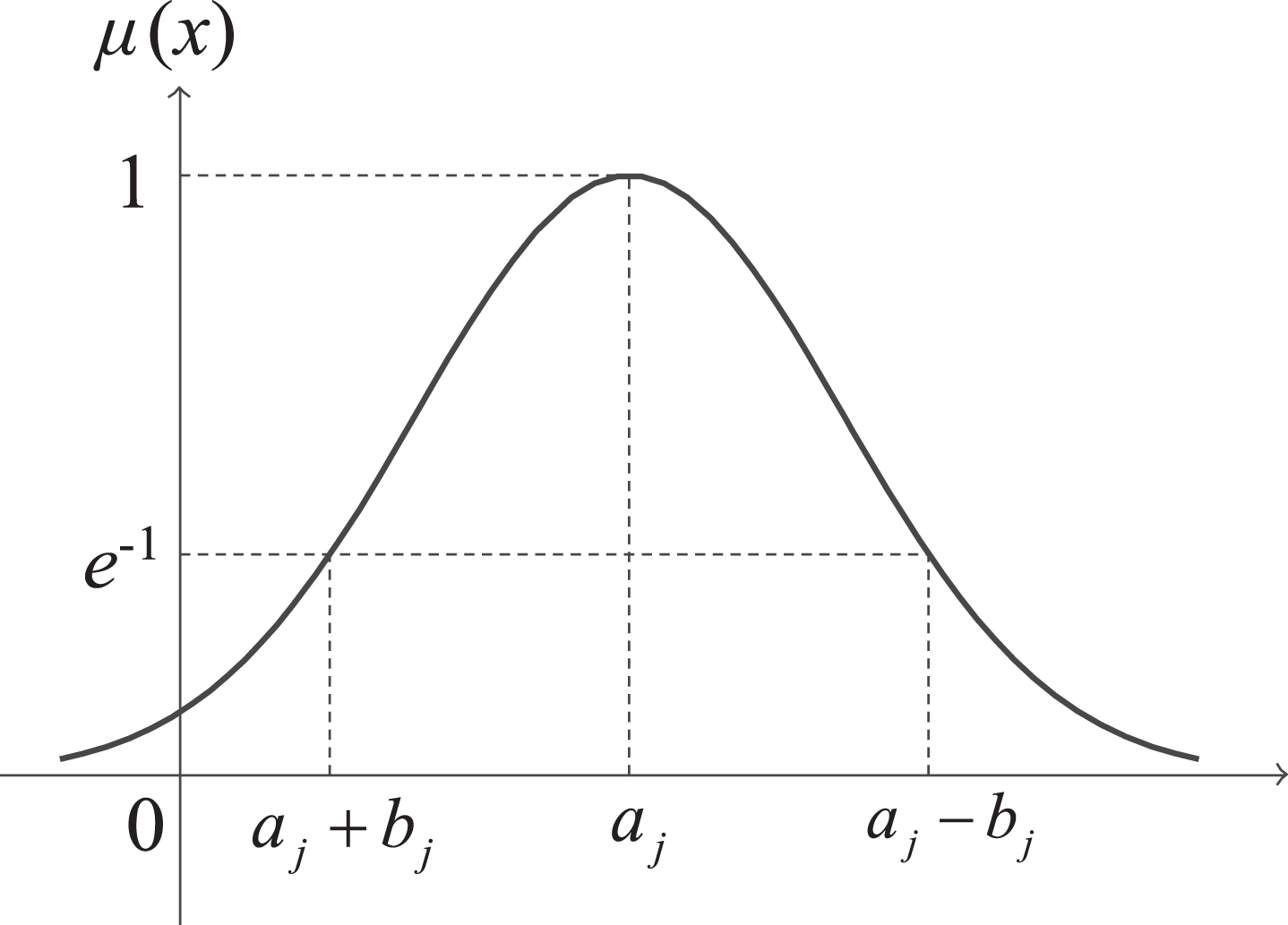
As it has been verified that GFN is more appropriate in air quality analysis by Wang et al. [16], the fuzzy coefficients in this paper are all assumed to be GFNs, denoted by $\tilde{A_{j}} = G (a_{j}, b_{j})$ , j = 0, 1, …, 5, whose membership functions are described as $μ (x) = e^{- {(\frac{x - a_{j}}{b_{j}})}^{2}},$ (3) where a_j is the expectation of $\tilde{A_{j}}$ , which is crisp parameters. In addition, b_j > 0 is the standard deviation of $\tilde{A_{j}}$ , which is also crisp parameters. And the shape function of the GFN is depicted as Figure 1.

Fig. 1

The membership function of the GFN ${\tilde{A}}_{j}$ .

Then, according to the linearity of the GFNs derived from Zadeh [11]’s extension principle, the estimated fuzzy AQI is also a GFN, and the FLR model can be expressed as $\begin{matrix} \begin{matrix} \tilde{y_{i}} & = G (a_{0}, b_{0}) x_{i 0} + G (a_{1}, b_{1}) x_{i 1} + G (a_{2}, b_{2}) x_{i 2} \\ + \dots + G (a_{5}, b_{5}) x_{i 5} \\ = G (a_{0} x_{i 0} + a_{1} x_{i 1} + a_{2} x_{i 2} + \dots + a_{5} x_{i 5}, \\ b_{0} x_{i 0} + b_{1} x_{i 1} + b_{2} x_{i 2} + \dots + b_{5} x_{i 5}) \\ = G (\sum_{j = 0}^{5} a_{j} x_{ij}, \sum_{j = 0}^{5} b_{j} x_{ij}) . \end{matrix} \end{matrix}$ (4) That is, the estimated fuzzy AQI, $\tilde{y_{i}}$ (i = 1, 2, …, m), is a GFN with the expectation and the most possible value of $\sum_{j = 0}^{5} a_{j} x_{ij}$ and the standard deviation of $\sum_{j = 0}^{5} b_{j} x_{ij}$ . Note that by conducting the curve fitting on pollutants, Wang et al. [16] has revealed that the membership function of the daily AQI is approximate to Gaussian distribution, which is consistent with the conclusion drawn from Eq. (B.2).

2.3 Tanaka’s FLR model using the minimum fuzziness criterion

Basically, there are two categories of fuzzy linear regression models among the numerous related research. The first one is the fuzzy regression using minimum fuzziness criterion which views the deviations in the observations as fuzziness of the model and focuses on finding fuzzy parameters minimizing the total spread of the parameters while keeping the feasibility of the possibilistic regression model by solving programming models [17 , 26]. And the second one aims at minimizing the total sum of squares of the errors, extending the least squares method of ordinary regression to the fuzzy environment [27 –29]. In both categories, the notion of "best fit" incorporates the functional optimization, therefore both were intensively applied. Due to the huge number of the observed and predicted values and the Gaussian fuzzy numbers involved in this paper, the least-squares based models would inevitably encounter the challenge of high computational complexity [30]. For this reason, Tanaka’s model is employed in this paper.

In the light of the minimum fuzziness criterion claimed by Tanaka [17], the objective of the FLR is to find out the fuzzy coefficients by minimizing the system fuzziness (or called total fuzziness [31]), symbolized by ▵, in line with the predetermined fuzziness parameter h (0 ≤ h ≤ 1), which denotes the degree of fitting of the model and is formally judged by domain researchers through experience and knowledge.

Analytically, the system fuzziness is a summation of the fuzziness of each estimated fuzzy output $\tilde{y_{i}}$ , i.e., $▵ = \sum_{i = 1}^{m} ▵ \tilde{y_{i}}, i = 1, 2, \dots, m,$ (5) where $▵ \tilde{y_{i}}$ is the area of $\tilde{y_{i}}$ that can be figured out by its membership function. Accordingly, with regard to the GFN, $\tilde{y_{i}} = G (α_{i}, β_{i})$ , the fuzziness can be expressed as $▵ \tilde{y_{i}} = \int_{- \infty}^{+ \infty} e^{- {(\frac{x - \sum_{j = 0}^{5} a_{j} x_{ij}}{\sum_{j = 0}^{5} b_{j} x_{ij}})}^{2}} dx = \sqrt{π} \sum_{j = 0}^{5} b_{j} x_{ij}$ (6) and thus the system fuzziness is derived as $▵ = \sum_{i = 1}^{m} ▵ \tilde{y_{i}} = \sqrt{π} \sum_{i = 1}^{m} \sum_{j = 0}^{5} b_{j} x_{ij} .$ (7)

{ On the other hand, following from the minimum fuzziness criterion, the FLR model is subject to the following inclusion condition: $y_{i} \in [\tilde{y_{i}}]^{h}, i = 1, 2, \dots, m,$ (8) where y_i is the observed value of the dependent variable, and $[\tilde{y_{i}}]^{h}$ is the h-level set of the estimated fuzzy output, $\tilde{y_{i}}$ , which can be calculated by Eqs. (3) and (B.2) as $\begin{array}{l} [\tilde{y_{i}}]^{h} = [\sum_{j = 0}^{5} a_{j} x_{i j} - \sqrt{- \ln h} \sum_{j = 0}^{5} b_{j} x_{i j}, \\ \sum_{j = 0}^{5} a_{j} x_{i j} + \sqrt{- \ln h} \sum_{j = 0}^{5} b_{j} x_{i j}], \end{array}$ (9) and then constraints (8) can be transformed into the following inequations, $\begin{matrix} \sum_{j = 0}^{5} a_{j} x_{ij} - \sqrt{- ln h} \sum_{j = 0}^{5} b_{j} x_{ij} \leq y_{i}, \\ - \sum_{j = 0}^{5} a_{j} x_{ij} - \sqrt{- ln h} \sum_{j = 0}^{5} b_{j} x_{ij} \leq - y_{i}, \\ i = 1, 2, \dots, m . \end{matrix}$ (10) Henceforth, the proposed FLR model is finally formulated as the following programming, $\begin{matrix} {\begin{matrix} min ▵ = \sqrt{π} \sum_{i = 1}^{m} \sum_{j = 0}^{5} b_{j} x_{ij} \\ subject to : \\ \sum_{j = 0}^{5} a_{j} x_{ij} - \sqrt{- ln h} \sum_{j = 0}^{5} b_{j} x_{ij} \leq y_{i}, \\ i = 1, 2, \dots, m \\ - \sum_{j = 0}^{5} a_{j} x_{ij} - \sqrt{- ln h} \sum_{j = 0}^{5} b_{j} x_{ij} \leq - y_{i}, \\ i = 1, 2, \dots, m \\ b_{j} > 0, j = 0, 1, \dots, 5, \end{matrix} \end{matrix}$ (11) where x_ij is the value of the aforementioned meteorological factor x_j released by the meteorological data center, y_i is the real daily AQI value, and a_j and b_j are the crisp parameters to be solved. It is obvious that by using the existing softwares such as Lingo and Matlab, model (11) definitely can be readily solved. After figuring out the crisp parameters, the FLR model (2) can be explicitly expressed, and with the officially released values, x_ij, the fuzzy AQI in the future can be predicted thence.

2.4 Performance validation

Once the FLR model is established, the predicted fuzzy AQI can be obtained and expressed by its membership function, and then the performance of the FLR model can be validated by prediction. Different from the result of the statistical regression, the predicted AQI of the FLR model is a fuzzy number containing multifaceted information, and the conventional methods for evaluation is no longer applicable. Therefore, three important measures were proposed in succession by the researchers with regard to the FLR model, as shown in Figure 2.

Fig. 2

The performance validation of the FLR model.

The first one is the membership degree of y_i with respect to $\tilde{y_{i}}$ , $μ_{\tilde{y_{i}}} (y_{i})$ , representing the possibility that the real value, y_i is achieved, with respect to the predicted value, $\tilde{y_{i}}$ . As we can see in Figure 2 Part I, a higher membership degree of $μ_{\tilde{y_{i}}} (y_{i})$ means that y_i is closer to a_i, the most possible value with $μ_{\tilde{y_{i}}} (a_{i}) = 1$ , and it is more likely that the model is of higher accuracy, regardless of the shape function of $\tilde{y_{i}}$ .

The second measure is the fuzziness of $\tilde{y_{i}}$ , i.e., $▵ \tilde{y_{i}}$ . In Tanaka’s FLR model, the deviations between the observed values and the estimated values are regarded as the fuzziness of the parameters of the system, which is vividly depicted as the area of the predicted value (see Figure 2 Part II). A fuzzy number with smaller fuzziness implies a narrower predicted interval, and thus the real value can be predicted with smaller uncertainty and higher determinacy when the membership degree of y_i is not considered.

Figure 2 shows that the membership degree and the fuzziness evaluate the performance of the FLR model from different dimensions, whereas Moskowitz and Kim [32] stated that as the h value increases, both the membership degree and the fuzziness may increase. Under this circumstance, utilizing them for evaluation may lead to contradictory conclusions, such that a model with a higher (lower) membership degree of $μ_{\tilde{y_{i}}} (y_{i})$ may also has larger (smaller) fuzziness of $\tilde{y_{i}}$ . To deal with this problem, Liu and Chen [33] introduced the third credibility measure z_i that divides the membership degree $μ_{\tilde{y_{i}}} (y_{i})$ by the fuzziness $▵ \tilde{y_{i}}$ (see Figure 2 Part III). They also pointed out that the higher z_i is, the better the performance of $\tilde{y_{i}}$ in representing y_i and the higher the reliability of the model will be, which has been verified while applying the measure in the quality function deployment [34, 35]. In the next sections, the process of validating the performance of the FLR models for predicting AQI based on the three measures will be illustrated in detail.

3 Illustrative Example

In this section, we are dedicated to establishing the FLR model of Shanghai as an example. After collecting the daily data of the meteorological factors and AQI, and verifying the seasonal effect graphically and statistically, four groups of fuzzy coefficients with respect to four seasons are obtained. And then, the coefficients are specifically analyzed on the basis of the existing literature together with the typical characteristics of Shanghai’s climatic environment to explain the reasonableness of the model.

3.1 Data collection

With 121°29’E and 31°14’N, Shanghai is located at the mouth of the Yangtze River Delta, surrounded by Zhejiang and Jiangsu provinces to the north, south and west, and bounded to the east by the East China Sea. Thanks to its special position, the city features a humid subtropical climate and experiences four distinct seasons, i.e., spring (March to May), summer (June to August), autumn (September to November), and winter (December to February), according to Chinese lunar calendar. On the other hand, as one of the four populous and important municipalities directly governed by the central administration in China, Shanghai has developed as an indispensable financial and technology center as well as the busiest container port in the world owning to its favourable geological conditions and years of policy support 1 , with over 10,000 factories. In the context of international environmental protection caused by climate warming, the increasingly serious air pollution issue accompanied by its population explosion, economic prosperity, and rapid urbanization has also been paid more and more attention. As reported, the air pollution of Shanghai was even worse than that of Beijing by the end of 2018, which is well known for its bad air quality. The typical weather, economic status, as well as the pollution level make the metropolis an excellent example in this paper. Consequently, the six dimensional data from March 2016 to February 2017 are collected for investigating the FLR model of Shanghai’s AQI on the five meteorological factors. Herein, the daily averaged temperature, relative humidity, wind speed, visibility, and sea-level pressure are from the website of National Scientific Meteorological Data Center 2 , and the daily AQI is from the website of Resources and Environment Data Cloud Platform 3 .

3.2 Basic statistical analysis

As mentioned above, Shanghai is a distinct seasonal city, the meteorological characteristics of which in the four seasons can be quite different from each other. With this consideration, we calculate the monthly mean values of the meteorological factors and AQI from March 2016 to February 2017, and depict them in Figure 3, from which we can see that all the factors experienced seasonal change except for wind speed. Therein, temperature and visibility had seen a similar and significant trend of increasing in summer and decreasing in autumn, whereas the trend of sea-level pressure was totally opposite, i.e., summer witnessed lower values than other seasons. Additionally, relative humidity fluctuated slightly on an annual basis and reached its peak in summer, and wind speed is hardly changed over the whole year. Correspondingly, AQI varies dramatically during the year, and the values in spring and winter are relatively high.

Fig. 3

The monthly values of meteorological factors and AQI (March 2016 - February 2017).

Afterwards, in order to further reveal the seasonal differences with more specific information, a one-way ANOVA using Scheffe’s method for multiple comparisons is conducted with the threshold of 0.05 regarding each variable, and the p-value of the pairwise comparisons are shown in Table 3. Apparently, all the values of temperature are 0.000, whereas the ones of wind speed are far greater than the predetermined p-value of 0.05, showing that temperature and wind speed are the factors with the most and least significant seasonal differences. As for the other factors and AQI, most of the values are smaller than 0.05, indicating that the differences are significant in certain seasons. The results are consistent with the trends shown in Figure 3. Consequently, in consideration of the seasonal effect in the meteorological factors and AQI, it is more reasonable to classify the six dimensional data into four groups by season and accordingly formulate four seasonal FLR models.

Table 3

ANOVA analyses regarding the meteorological factors and AQI

	AQI				T				RH
	Spr.	Sum.	Aut.	Win.	Spr.	Sum.	Aut.	Win.	Spr.	Sum.	Aut.	Win.
Spr.	-	0 . 000^*	0 . 000^*	0.510	-	0 . 000^*	0 . 000^*	0 . 000^*	-	0.206	0 . 021^*	0.494
Sum.	0 . 000^*	-	0.907	0 . 009^*	0 . 000^*	-	0 . 000^*	0 . 000^*	0.206	-	0.802	0 . 000^*
Aut.	0 . 000^*	0.907	-	0 . 001^*	0 . 000^*	0 . 000^*	-	0 . 000^*	0 . 021^*	0.802	-	0 . 000^*
Win.	0.510	0.009*	0 . 001^*	-	0 . 000^*	0 . 000^*	0 . 000^*	-	0.494	0 . 004^*	0 . 000^*	-
	WS				V				SLP
	Spr.	Sum.	Aut.	Win.	Spr.	Sum.	Aut.	Win.	Spr.	Sum.	Aut.	Win.
Spr.	-	0.122	0.726	0.744	-	0 . 000^*	0 . 005^*	0.983	-	0 . 000^*	0.066	0 . 000^*
Sum.	0.122	-	0.660	0.644	0 . 000^*	-	0.310	0 . 000^*	0 . 000^*	-	0 . 000^*	0 . 000^*
Aut.	0.726	0.660	-	1.000	0 . 005^*	0.310	-	0 . 001^*	0.066	0 . 000^*	-	0 . 000^*
Win.	0.744	0.644	1.000	-	0.983	0 . 000^*	0 . 001^*	-	0 . 000^*	0 . 000^*	0 . 000^*	-

^*: Difference is significant between corresponding seasons with regard to the same variable (at p ≤ 0.05).

3.3 Modeling and parameters analyses

As an important parameter measuring the degree of the fitting of the FLR model, h constrains the upper and lower bounds of the observed crisp output values and directly affects the reliability of the derived fuzzy outputs [17, 19]. It is generally preselected by decision makers subjectively based on the specific characteristics of certain problem. In the previous studies, there are various h values, such as 0, 0.5, 0.8 and 0.9 [17 , 37]. Since we expect to predicted AQI with higher reliability, a high h value of 0.8 is selected. Besides, the most commonly used and moderate value, 0.5, is also chosen for comparison.

By setting the h value as 0.8 and 0.5, respectively, and solving model (11) with the data sources above using Matlab 2016a, the fuzzy parameters $\tilde{A_{j}} = G (a_{j}, b_{j}), j = 0, 1, \dots, 5,$ of model (2) are obtained and listed in Table 4, where a_j and b_j stand for the expectation and standard deviation of $\tilde{y_{i}}$ . First, as we can see, the two groups of results share the similar characteristics that there are seven b_j significantly different from 0, exemplifying the fuzziness of the relationship between certain meteorological factors and AQI in certain seasons. Then, in order to fully understand the correlation between each meteorological factor and AQI in Shanghai, the values of a_j, j = 0, 1, …, 5, i.e., the most possible coefficients with the membership degree of 1, are analyzed in great detail as follows.

As shown in Table 4, the values of a₂ and a₄ are all negative, indicating a negative relationship between AQI and relative humidity as well as visibility all through the year, which is consistent with most studies. By comparison, the result of the relationship between temperature/wind speed/sea-level pressure and AQI is complex and inconsistent with others.

Table 4
The fuzzy coefficients of four seasonal GFN models with h = 0.8 and h = 0.5

Variable Coefficients Spring Summer Autumn Winter

a _j b _j a _j b _j a _j b _j a _j b _j

h=0.8 $\tilde{A_{0}} = G (a_{0}, b_{0})$ 998.23 0.00 -1705.90 0.00 2722.82 0.00 -1587.15 0.00

x₁ (T) $\tilde{A_{1}} = G (a_{1}, b_{1})$ 0.73 2.56 0.60 0.00 -1.92 0.00 1.63 0.00

x₂ (RH) $\tilde{A_{2}} = G (a_{2}, b_{2})$ -0.67 0.11 -1.37 0.82 -1.33 1.13 -0.83 0.00

x₃ (WS) $\tilde{A_{3}} = G (a_{3}, b_{3})$ 2.21 5.49 -4.09 0.00 -0.54 0.00 1.63 3.26

x₄ (V) $\tilde{A_{4}} = G (a_{4}, b_{4})$ -0.54 0.53 -3.20 0.00 -3.04 0.00 -6.20 0.00

x₅ (SLP) $\tilde{A_{5}} = G (a_{5}, b_{5})$ -0.86 0.00 1.92 0.00 -2.42 0.00 1.71 0.00

h=0.5 $\tilde{A_{0}} = G (a_{0}, b_{0})$ 998.23 0.00 -1705.90 0.00 2722.82 0.00 -1587.15 0.00

x₁ (T) $\tilde{A_{1}} = G (a_{1}, b_{1})$ 0.73 1.45 0.60 0.00 -1.92 0.00 1.63 0.00

x₂ (RH) $\tilde{A_{2}} = G (a_{2}, b_{2})$ -0.67 0.07 -1.37 0.47 -1.33 0.64 -0.83 0.00

x₃ (WS) $\tilde{A_{3}} = G (a_{3}, b_{3})$ 2.21 3.11 -4.09 0.00 -0.54 0.00 1.63 1.61

x₄ (V) $\tilde{A_{4}} = G (a_{4}, b_{4})$ -0.54 0.30 -3.20 0.00 -3.04 0.00 -6.20 0.00

x₅ (SLP) $\tilde{A_{5}} = G (a_{5}, b_{5})$ -0.86 0.00 1.92 0.00 -2.42 0.00 1.71 0.05

	Variable	Coefficients	Spring	Summer	Autumn	Winter
h=0.8		$\tilde{A_{0}} = G (a_{0}, b_{0})$	998.23	0.00	-1705.90	0.00	2722.82	0.00	-1587.15	0.00
	x₁ (T)	$\tilde{A_{1}} = G (a_{1}, b_{1})$	0.73	2.56	0.60	0.00	-1.92	0.00	1.63	0.00
	x₂ (RH)	$\tilde{A_{2}} = G (a_{2}, b_{2})$	-0.67	0.11	-1.37	0.82	-1.33	1.13	-0.83	0.00
	x₃ (WS)	$\tilde{A_{3}} = G (a_{3}, b_{3})$	2.21	5.49	-4.09	0.00	-0.54	0.00	1.63	3.26
	x₄ (V)	$\tilde{A_{4}} = G (a_{4}, b_{4})$	-0.54	0.53	-3.20	0.00	-3.04	0.00	-6.20	0.00
	x₅ (SLP)	$\tilde{A_{5}} = G (a_{5}, b_{5})$	-0.86	0.00	1.92	0.00	-2.42	0.00	1.71	0.00
h=0.5		$\tilde{A_{0}} = G (a_{0}, b_{0})$	998.23	0.00	-1705.90	0.00	2722.82	0.00	-1587.15	0.00
	x₁ (T)	$\tilde{A_{1}} = G (a_{1}, b_{1})$	0.73	1.45	0.60	0.00	-1.92	0.00	1.63	0.00
	x₂ (RH)	$\tilde{A_{2}} = G (a_{2}, b_{2})$	-0.67	0.07	-1.37	0.47	-1.33	0.64	-0.83	0.00
	x₃ (WS)	$\tilde{A_{3}} = G (a_{3}, b_{3})$	2.21	3.11	-4.09	0.00	-0.54	0.00	1.63	1.61
	x₄ (V)	$\tilde{A_{4}} = G (a_{4}, b_{4})$	-0.54	0.30	-3.20	0.00	-3.04	0.00	-6.20	0.00
	x₅ (SLP)	$\tilde{A_{5}} = G (a_{5}, b_{5})$	-0.86	0.00	1.92	0.00	-2.42	0.00	1.71	0.05

Specifically, it seems to be a positive relationship between temperature and AQI, but that of autumn is an exception. The abnormal phenomena can be ascribed to atmospheric inversion [38]. Generally, temperature decreases with the increase of altitude which is negatively related to the air density. As a consequence, the rise of temperature in the lower atmosphere regularly causes a gradual decline in the air density of ground layer, and the atmosphere then turns into a top-heavy structure in which the airflow is unstable and easy to form convection, whirling and sweeping away contaminants on the surface and bringing a temporary reduction in pollutant concentrations. However, when atmospheric inversion occurs, the air near the earth’s surface is forced to spread down rather than up, and thereby aggravate the air pollution. Actually, atmospheric inversion often happens in Shanghai except autumn [18], it is why the temperature has a positive relationship with AQI in spring, summer, and winter, but a negative one in autumn.

WindTable 4). The result is due to the special geographical location of Shanghai. As pictured in Figure 4(a), Shanghai is a large city with numerous industrial parks and, consequently, has several areas with many pollution sources. Conspicuously, a stronger wind can blow away more pollutants the city itself produces and result in a lower AQI, so the correlation is ought to be negative, as Figure 3(b) shows that the wind speed in spring and winter of 2016-2017 in Shanghai is larger than that in summer and autumn on the whole. Nevertheless, as mentioned before, Shanghai is a city with unique geographical conditions and surrounding environment, and the wind direction changes remarkably in different seasons, especially in summer and winter (Figure 4(b)) [39, 40]. To be specific, in summer, the air travels almost from the southeast direction. A moist breeze from the East China Sea is likely to be responsible for the reduction of AQI. Yet the prevailing wind in winter are mainly from the northwest area. Before arriving, the wind usually passes through Zhejiang and Jiangsu Province, fertile areas for industry and manufacturing as well as the major pollution sources in the southeastern China. Hence, the wind would inevitably bring in pollutants and increase AQI. This well explains why the correlation is positive in spring and winter but negative in summer and autumn.

Fig. 4

The distribution of pollution sources 4 and wind direction in Shanghai.

Studies on the relationship between AQI and sea-level pressure have drawn controversial conclusions for several years, and in this paper the relationship is also complex and elusive. It is beyond doubt that airflow tends to move along the direction that pressure decreases which is significantly affected by the rise of elevation. Thus, it would circle more frequently and vigorously in lower atmosphere, generating strong wind and heavy rainfall which can rapidly lower pollutant concentrations. But sometimes slow airflow may stay in an area for a long time, so that it not only cannot clean pollutants away, but is more likely to bring them back to the ground from the upper air. According to the complexity of the atmosphere, this phenomenon is really possible to occur, and further analyses should be conducted in the future. Figure 5 concludes various kinds of relationships between the meteorological factors and AQI.

Fig. 5

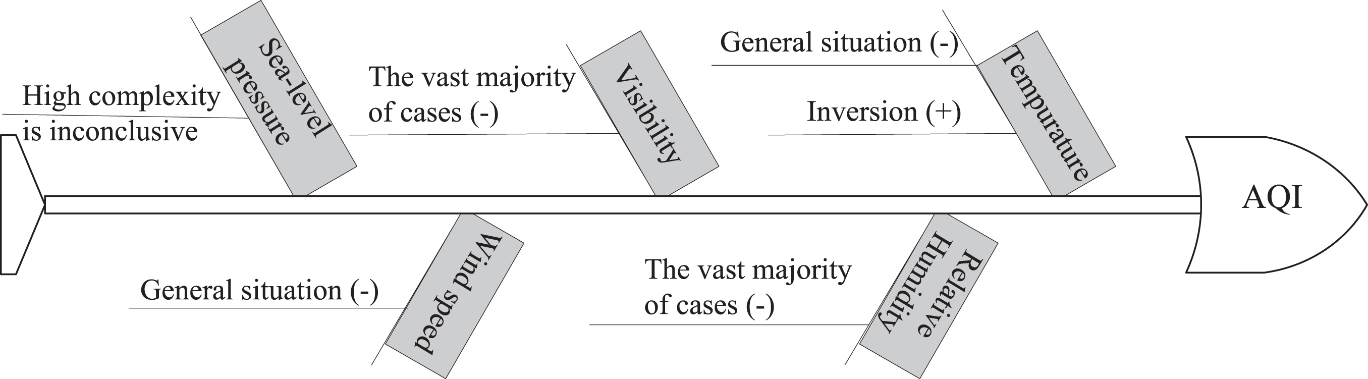
The relationships between AQI and the meteorological factors.

Above all, owing to the special geographical location of Shanghai, the climatic environment in each season is quite different, and therefore the relationship between the meteorological factors and AQI is no longer simply positive or negative. The results precisely justify that it is a better way to establish the FLR models by season for such a special city.

4 Validation and Comparison

In this section, we first validate the performance of the four seasonal FLR models in Shanghai via the data from March 2017 to February 2018, and then compare it with the models based on the commonly used TFN by using the three measures proposed in Section 2.4, i.e., membership degree, fuzziness and credibility, on a monthly and daily basis.

4.1 Model verification

In Sections 2 and 3, the FLR models for different seasons in Shanghai have been explicitly expressed and statistically analyzed in detail, and in this section four seasonal models are used for prediction with the data of the next year. The specific steps include: First, we classify necessarily the daily average values of the five meteorological factors into four groups in terms of seasons and plug them into the four FLR models with the fuzzy coefficients in Table 4, respectively, and figure out 365 fuzzy daily AQI, $\tilde{y_{i}}$ , i = 1, 2, …, 365, as GFNs. Afterwards, compare the predicted AQI with the real data obtained from the official website, y_i, by calculating the membership degree of y_i with respect to $\tilde{y_{i}}$ , denoted by $μ_{\tilde{y_{i}}} (y_{i})$ , which represents the occurrence possibility of the real value corresponding to $\tilde{y_{i}}$ . Generally, the higher $μ_{\tilde{y_{i}}} (y_{i})$ is, the more likely it is the models will predict the real value, and the higher the predicting accuracy of the models is. The results are recorded in tables and figures, where the information of summer 2017 is shown in Table 5 and Figures 6-7 as an example for further analysis, and the rest is presented in Appendix 5.

Table 5
The real values of daily AQI (y_i) and the corresponding membership degrees ( $μ_{\tilde{y_{i}}} (y_{i})$ ) in summer 2017 by the GFN model

Date y _i $μ_{\tilde{y_{i}}} (y_{i})$ Date y _i $μ_{\tilde{y_{i}}} (y_{i})$ Date y _i $μ_{\tilde{y_{i}}} (y_{i})$

h = 0.8 h = 0.5 h = 0.8 h = 0.5 h = 0.8 h = 0.5

6/1 110 0.89 0.70 7/1 77 0.87 0.65 8/1 45 0.84 0.58

6/2 93 0.22 0.01 7/2 41 1.00 0.99 8/2 41 0.93 0.79

6/3 60 0.65 0.26 7/3 55 0.95 0.85 8/3 74 0.96 0.89

6/4 60 0.44 0.08 7/4 43 0.99 0.98 8/4 84 0.96 0.89

6/5 55 0.96 0.88 7/5 64 0.98 0.94 8/5 83 1.00 0.99

6/6 54 0.97 0.91 7/6 66 0.98 0.93 8/6 136 0.71 0.15

6/7 89 0.89 0.70 7/7 68 0.95 0.86 8/7 132 0.85 0.25

6/8 138 0.81 0.53 7/8 66 0.87 0.66 8/8 59 0.97 0.44

6/9 112 0.97 0.91 7/9 47 0.97 0.13 8/9 33 1.00 0.98

6/10 44 0.98 0.94 7/10 44 0.97 0.90 8/10 84 1.00 1.00

6/11 53 0.89 0.71 7/11 61 0.95 0.86 8/11 126 0.95 0.21

6/12 54 0.81 0.52 7/12 90 1.00 0.99 8/12 76 1.00 0.99

6/13 46 0.83 0.57 7/13 97 0.96 0.88 8/13 55 0.97 0.91

6/14 46 0.97 0.92 7/14 95 0.99 0.96 8/14 41 0.98 0.94

6/15 62 0.71 0.35 7/15 86 0.95 0.47 8/15 92 1.00 0.99

6/16 70 0.97 0.90 7/16 74 0.87 0.65 8/16 67 0.91 0.76

6/17 76 0.91 0.75 7/17 44 0.98 0.93 8/17 64 1.00 0.99

6/18 56 0.98 0.94 7/18 86 1.00 0.99 8/18 78 0.89 0.71

6/19 43 0.94 0.84 7/19 95 0.96 0.88 8/19 87 0.98 0.19

6/20 46 1.00 0.99 7/20 103 0.99 0.35 8/20 40 0.95 0.85

6/21 51 0.99 0.98 7/21 116 1.00 0.46 8/21 54 1.00 1.00

6/22 43 0.99 0.98 7/22 115 0.95 0.86 8/22 25 0.89 0.71

6/23 74 1.00 1.00 7/23 116 1.00 0.41 8/23 34 0.86 0.64

6/24 47 0.94 0.83 7/24 121 0.93 0.81 8/24 58 0.95 0.87

6/25 66 1.00 1.00 7/25 112 0.64 0.25 8/25 60 0.95 0.86

6/26 116 0.91 0.75 7/26 96 0.99 0.96 8/26 53 1.00 0.38

6/27 127 0.87 0.65 7/27 80 1.00 0.99 8/27 47 0.87 0.67

6/28 82 0.99 0.98 7/28 36 0.99 0.98 8/28 63 0.98 0.94

6/29 52 0.98 0.95 7/29 30 0.92 0.77 8/29 45 0.88 0.67

6/30 60 0.94 0.82 7/30 33 0.90 0.72 8/30 41 0.86 0.64

7/31 39 0.90 0.72 8/31 57 0.84 0.59

Date	y _i	$μ_{\tilde{y_{i}}} (y_{i})$	Date	y _i	$μ_{\tilde{y_{i}}} (y_{i})$	Date	y _i	$μ_{\tilde{y_{i}}} (y_{i})$
6/1	110	0.89	0.70	7/1	77	0.87	0.65	8/1	45	0.84	0.58
6/2	93	0.22	0.01	7/2	41	1.00	0.99	8/2	41	0.93	0.79
6/3	60	0.65	0.26	7/3	55	0.95	0.85	8/3	74	0.96	0.89
6/4	60	0.44	0.08	7/4	43	0.99	0.98	8/4	84	0.96	0.89
6/5	55	0.96	0.88	7/5	64	0.98	0.94	8/5	83	1.00	0.99
6/6	54	0.97	0.91	7/6	66	0.98	0.93	8/6	136	0.71	0.15
6/7	89	0.89	0.70	7/7	68	0.95	0.86	8/7	132	0.85	0.25
6/8	138	0.81	0.53	7/8	66	0.87	0.66	8/8	59	0.97	0.44
6/9	112	0.97	0.91	7/9	47	0.97	0.13	8/9	33	1.00	0.98
6/10	44	0.98	0.94	7/10	44	0.97	0.90	8/10	84	1.00	1.00
6/11	53	0.89	0.71	7/11	61	0.95	0.86	8/11	126	0.95	0.21
6/12	54	0.81	0.52	7/12	90	1.00	0.99	8/12	76	1.00	0.99
6/13	46	0.83	0.57	7/13	97	0.96	0.88	8/13	55	0.97	0.91
6/14	46	0.97	0.92	7/14	95	0.99	0.96	8/14	41	0.98	0.94
6/15	62	0.71	0.35	7/15	86	0.95	0.47	8/15	92	1.00	0.99
6/16	70	0.97	0.90	7/16	74	0.87	0.65	8/16	67	0.91	0.76
6/17	76	0.91	0.75	7/17	44	0.98	0.93	8/17	64	1.00	0.99
6/18	56	0.98	0.94	7/18	86	1.00	0.99	8/18	78	0.89	0.71
6/19	43	0.94	0.84	7/19	95	0.96	0.88	8/19	87	0.98	0.19
6/20	46	1.00	0.99	7/20	103	0.99	0.35	8/20	40	0.95	0.85
6/21	51	0.99	0.98	7/21	116	1.00	0.46	8/21	54	1.00	1.00
6/22	43	0.99	0.98	7/22	115	0.95	0.86	8/22	25	0.89	0.71
6/23	74	1.00	1.00	7/23	116	1.00	0.41	8/23	34	0.86	0.64
6/24	47	0.94	0.83	7/24	121	0.93	0.81	8/24	58	0.95	0.87
6/25	66	1.00	1.00	7/25	112	0.64	0.25	8/25	60	0.95	0.86
6/26	116	0.91	0.75	7/26	96	0.99	0.96	8/26	53	1.00	0.38
6/27	127	0.87	0.65	7/27	80	1.00	0.99	8/27	47	0.87	0.67
6/28	82	0.99	0.98	7/28	36	0.99	0.98	8/28	63	0.98	0.94
6/29	52	0.98	0.95	7/29	30	0.92	0.77	8/29	45	0.88	0.67
6/30	60	0.94	0.82	7/30	33	0.90	0.72	8/30	41	0.86	0.64
				7/31	39	0.90	0.72	8/31	57	0.84	0.59

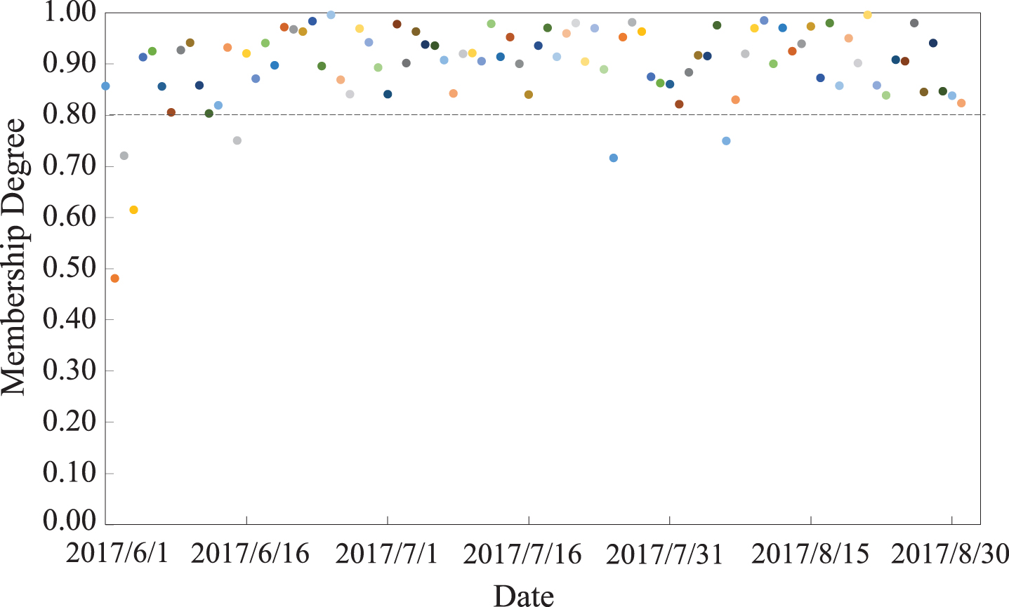
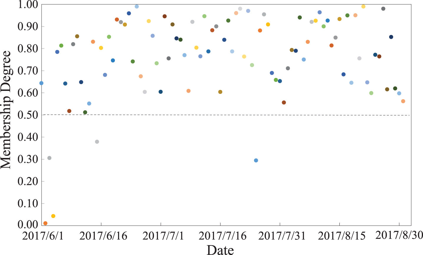
It can be seen apparently from Figures 6-7 that the large majority of the points (86/87 out of 92) are located above the dotted line with the membership degree of 0.8/0.5, the h values set for solving the FLR models using the minimum fuzziness criterion, and the average membership degree is 0.92/0.76, showing the well predicting effectiveness of the model for summer. Several points below 0.8/0.5 could be ascribed to the complexity of atmosphere system and changeable pollutant emissions. For example, the two days in June with the extremely low value are due to the abnormal change of relative humidity and visibility during that time. The similar results can also be observed in other seasons, for more details, please refer to Appendix 5.

Fig. 6

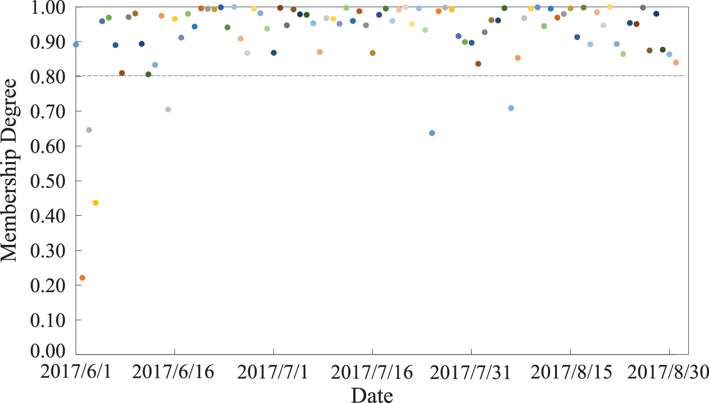
The scatter diagram of the membership degrees in summer 2017 by the GFN model with h = 0.8.

Fig. 7

The scatter diagram of the membership degrees in summer 2017 by the GFN model with h = 0.5.

Noticeably, in the above experiment, one day’s AQI is predicted on the basis of the values of the meteorological factors on that very day, which are not readily available and can only be replaced by the ones forecasted at least one day in advance in practice. Fortunately, it has been demonstrated that the forecast accuracy of these meteorological factors is up to 90% [41]. Hence, it can be concluded that the prediction results are credible and meaningful.

4.2 Comparisons between the GFN model and the TFN model

In the field of fuzzy applications, TFN has been extensively used for decades due to its simplicity, maturity, and ubiquity [42, 43]. Nevertheless, researchers in growing numbers, like Khan [44], have found that sometimes GFN is more suitable in describing a series of complicated or nonlinear membership functions. As a consequence, in order to make the prediction more persuasive, the FLR model based on symmetric TFNs (short for TFN model hereafter) is also analyzed for comparison. As elaborated in Appendix 5, the generalized TFN model is established and converted into a linear programming model by employing the minimum fuzziness criterion. Then, based on the data from March 2016 to February 2017, four seasonal TFN models are obtained. Table 6 shows triangular fuzzy coefficients, $\tilde{A_{j}} = T (c_{j}, d_{j})$ , j = 0, 1, …, 5. After that, the membership degrees of realistic AQI, y_i, from March 2017 to February 2018 are figured out and displayed. In the same way, the data in summer 2017 are illustrated in Table 7 for comparison, and the rest information are summarized in Appendix 5.

Table 6
The fuzzy coefficients of four seasonal TFN models with h = 0.8 and h = 0.5

Variable Coefficients Spring Summer Autumn Winter

c _j d _j c _j d _j c _j d _j c _j d _j

h=0.8 x ₀ $\tilde{A_{0}} = T (c_{0}, d_{0})$ 998.23 0.00 -1705.90 0.00 2722.82 0.00 -1587.15 0.00

x ₁ $\tilde{A_{1}} = T (c_{1}, d_{1})$ 0.73 6.04 0.60 0.00 -1.92 0.00 1.63 0.00

x ₂ $\tilde{A_{2}} = T (c_{2}, d_{2})$ -0.67 0.27 -1.37 1.94 -1.33 2.66 -0.83 0.00

x ₃ $\tilde{A_{3}} = T (c_{3}, d_{3})$ 2.21 12.96 -4.09 0.00 -0.54 0.00 1.63 7.69

x ₄ $\tilde{A_{4}} = T (c_{4}, d_{4})$ -0.54 1.25 -3.20 0.00 -3.04 0.00 -6.20 0.00

x ₅ $\tilde{A_{5}} = T (c_{5}, d_{5})$ -0.86 0.00 1.92 0.00 -2.42 0.00 1.71 0.00

h=0.5 x ₀ $\tilde{A_{0}} = T (c_{0}, d_{0})$ 998.23 0.00 -1705.90 0.00 2722.82 0.00 -1587.15 0.00

x ₁ $\tilde{A_{1}} = T (c_{1}, d_{1})$ 0.73 2.42 0.60 0.00 -1.92 0.00 1.63 0.00

x ₂ $\tilde{A_{2}} = T (c_{2}, d_{2})$ -0.67 0.11 -1.37 0.78 -1.33 1.06 -0.83 0.00

x ₃ $\tilde{A_{3}} = T (c_{3}, d_{3})$ 2.21 5.18 -4.09 0.00 -0.54 0.00 1.63 3.08

x ₄ $\tilde{A_{4}} = T (c_{4}, d_{4})$ -0.54 0.50 -3.20 0.00 -3.04 0.00 -6.20 0.00

x ₅ $\tilde{A_{5}} = T (c_{5}, d_{5})$ -0.86 0.00 1.92 0.00 -2.42 0.00 1.71 0.08

	Variable	Coefficients	Spring	Summer	Autumn	Winter
h=0.8	x ₀	$\tilde{A_{0}} = T (c_{0}, d_{0})$	998.23	0.00	-1705.90	0.00	2722.82	0.00	-1587.15	0.00
	x ₁	$\tilde{A_{1}} = T (c_{1}, d_{1})$	0.73	6.04	0.60	0.00	-1.92	0.00	1.63	0.00
	x ₂	$\tilde{A_{2}} = T (c_{2}, d_{2})$	-0.67	0.27	-1.37	1.94	-1.33	2.66	-0.83	0.00
	x ₃	$\tilde{A_{3}} = T (c_{3}, d_{3})$	2.21	12.96	-4.09	0.00	-0.54	0.00	1.63	7.69
	x ₄	$\tilde{A_{4}} = T (c_{4}, d_{4})$	-0.54	1.25	-3.20	0.00	-3.04	0.00	-6.20	0.00
	x ₅	$\tilde{A_{5}} = T (c_{5}, d_{5})$	-0.86	0.00	1.92	0.00	-2.42	0.00	1.71	0.00
h=0.5	x ₀	$\tilde{A_{0}} = T (c_{0}, d_{0})$	998.23	0.00	-1705.90	0.00	2722.82	0.00	-1587.15	0.00
	x ₁	$\tilde{A_{1}} = T (c_{1}, d_{1})$	0.73	2.42	0.60	0.00	-1.92	0.00	1.63	0.00
	x ₂	$\tilde{A_{2}} = T (c_{2}, d_{2})$	-0.67	0.11	-1.37	0.78	-1.33	1.06	-0.83	0.00
	x ₃	$\tilde{A_{3}} = T (c_{3}, d_{3})$	2.21	5.18	-4.09	0.00	-0.54	0.00	1.63	3.08
	x ₄	$\tilde{A_{4}} = T (c_{4}, d_{4})$	-0.54	0.50	-3.20	0.00	-3.04	0.00	-6.20	0.00
	x ₅	$\tilde{A_{5}} = T (c_{5}, d_{5})$	-0.86	0.00	1.92	0.00	-2.42	0.00	1.71	0.08

Table 7

The real values of daily AQI (y_i) and the corresponding membership degrees ( $μ_{\tilde{y_{i}}} (y_{i})$ ) in summer 2017 by the TFN model

Date	y _i	$μ_{\tilde{y_{i}}} (y_{i})$		Date	y _i	$μ_{\tilde{y_{i}}} (y_{i})$		Date	y _i	$μ_{\tilde{y_{i}}} (y_{i})$
		h = 0.8	h = 0.5			h = 0.8	h = 0.5			h = 0.8	h = 0.5
6/1	110	0.86	0.64	7/1	77	0.84	0.60	8/1	45	0.82	0.56
6/2	93	0.48	0.01	7/2	41	0.98	0.95	8/2	41	0.88	0.71
6/3	60	0.72	0.31	7/3	55	0.90	0.76	8/3	74	0.92	0.79
6/4	60	0.62	0.04	7/4	43	0.96	0.91	8/4	84	0.92	0.79
6/5	55	0.91	0.78	7/5	64	0.94	0.85	8/5	83	0.98	0.94
6/6	54	0.92	0.81	7/6	66	0.94	0.84	8/6	136	0.75	0.75
6/7	89	0.86	0.64	7/7	68	0.91	0.77	8/7	132	0.83	0.83
6/8	138	0.81	0.52	7/8	66	0.84	0.61	8/8	59	0.92	0.92
6/9	112	0.93	0.82	7/9	47	0.92	0.92	8/9	33	0.97	0.93
6/10	44	0.94	0.85	7/10	44	0.92	0.80	8/10	84	0.99	0.96
6/11	53	0.86	0.65	7/11	61	0.91	0.76	8/11	126	0.90	0.90
6/12	54	0.80	0.51	7/12	90	0.98	0.95	8/12	76	0.97	0.93
6/13	46	0.82	0.55	7/13	97	0.91	0.79	8/13	55	0.92	0.81
6/14	46	0.93	0.83	7/14	95	0.95	0.88	8/14	41	0.94	0.85
6/15	62	0.75	0.38	7/15	86	0.90	0.90	8/15	92	0.97	0.93
6/16	70	0.92	0.80	7/16	74	0.84	0.60	8/16	67	0.87	0.68
6/17	76	0.87	0.68	7/17	44	0.94	0.84	8/17	64	0.98	0.95
6/18	56	0.94	0.85	7/18	86	0.97	0.93	8/18	78	0.86	0.65
6/19	43	0.90	0.75	7/19	95	0.91	0.79	8/19	87	0.95	0.95
6/20	46	0.97	0.93	7/20	103	0.96	0.96	8/20	40	0.90	0.76
6/21	51	0.97	0.92	7/21	116	0.98	0.98	8/21	54	1.00	0.99
6/22	43	0.96	0.91	7/22	115	0.90	0.76	8/22	25	0.80	0.65
6/23	74	0.98	0.96	7/23	116	0.97	0.97	8/23	34	0.84	0.60
6/24	47	0.90	0.74	7/24	121	0.89	0.72	8/24	58	0.91	0.77
6/25	66	1.00	0.99	7/25	112	0.72	0.29	8/25	60	0.91	0.76
6/26	116	0.87	0.67	7/26	96	0.95	0.88	8/26	53	0.98	0.98
6/27	127	0.84	0.60	7/27	80	0.98	0.95	8/27	47	0.85	0.62
6/28	82	0.97	0.92	7/28	36	0.96	0.91	8/28	63	0.94	0.85
6/29	52	0.94	0.86	7/29	30	0.88	0.69	8/29	45	0.85	0.62
6/30	60	0.89	0.73	7/30	33	0.86	0.66	8/30	41	0.84	0.60
				7/31	39	0.86	0.65	8/31	57	0.82	0.56

Comparatively, a seemingly superficial consequence is presented: all the mean values in Tables 4 and 6 are equal, indicating that the most possible predicted values obtained by the GFN and symmetric TFN models (with the membership degree of 1) are exactly the same. Besides, the points in Figures 6 and 8 share similar distribution that only six out of 92 are below h = 0.8, illustrating that there appears to be no significant difference between the performance of the two classes of models. The same conclusion can be drawn in the case of h = 0.5, see Figures 7 and 9.

Fig. 8

The scatter diagram of the membership degrees in summer 2017 by the TFN model at h = 0.8.

Fig. 9

The scatter diagram of the membership degrees in summer 2017 by the TFN model at h = 0.5.

For further and deeper comparisons, the three measures discussed in Section 2.4 are employed herein. Owing to the large sample size of these 365-day data, the measures are calculated and presented by month in Figures 8-13 to facilitate more intuitionistic analyses.

A. Cumulative membership degree

As mentioned in Section 2.4, the membership degree of the observed daily AQI with respect to the predicted fuzzy number measures the accuracy of an FLR model regardless of the fuzziness of the model (see Figure 2 Part I for more details). After calculating and adding up all the membership degrees by month, we picture the monthly cumulative membership degree in Figure 10. It shows clearly that in each month, the bar in dark blue representing the results obtained by the GFN model is longer than that in light blue which stands for the corresponding result obtained by the TFN model. And numerically, in terms of accuracy, represented by the seasonal cumulative membership degree, the performance of the GFN models are, respectively, 2.04%, 2.59%, 3.03%, and 3.10% 4 higher.

Fig. 10

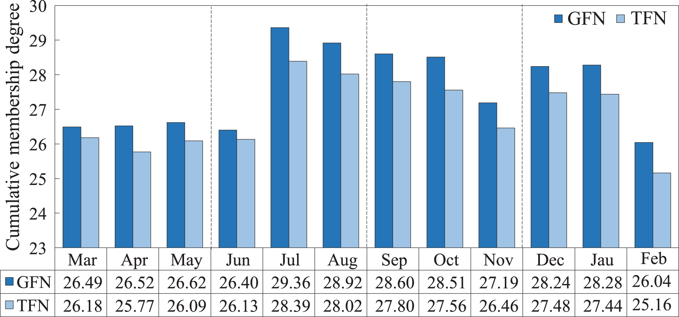
The monthly cumulative membership degrees from March 2017 to February 2018.

On the other hand, as shown in Figure 11, we count the number of days on which the membership degree of the real AQI, μ, is greater than or equal to 0.8 in each month and classify them into two categories, i.e., μ ≥ 0.9 and 0.8 ≤ μ < 0.9. It shows that although the two classes of models derive same number of days satisfying μ ≥ 0.8, the number of days satisfying μ ≥ 0.9 derived from the GFN models (bars with flash on the right) is always more than that of the TFN models (bars with slash on the left). For each season, the proportion of them, i.e., the number of days satisfying μ ≥ 0.9 obtained by the two classes of models (GFN/TFN) is 168.42%, 118.18%, 151.16%, 144.74%, respectively.

Fig. 11

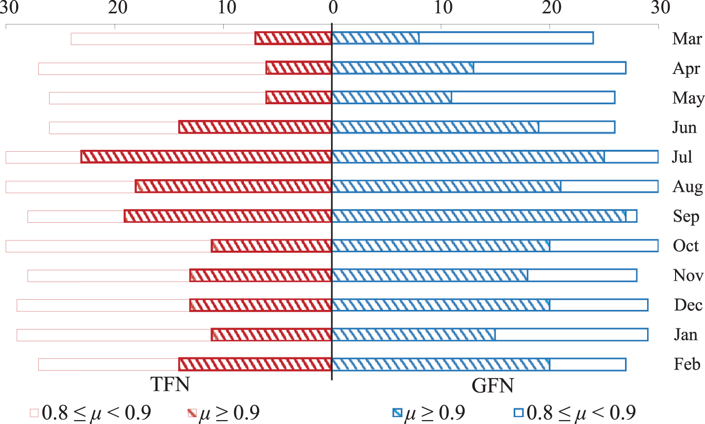
The number of days satisfying μ ≥ 0.8 in each month.

Furthermore, in order to compare the two classes of models in more detail, the membership degree of the daily data in April 2017 has been randomly selected, and predicted daily AQI’s membership functions, ${\tilde{y}}_{i}$ , are thoroughly pictured in Appendix 5, with the points in red representing the membership degrees of the real AQI with respect to the predicted fuzzy numbers. As the figures shown, the red points of the GFN models are always higher than the corresponding ones of the TFN models, meaning that the membership degrees of the predicted daily AQI obtained by the GFN models are higher while compared with the results of the TFN models.

To sum up, the histogram, the bar charts, and the figures of April 2017 work together to demonstrate that the accuracy of the GFN models is much better than that of the TFN models in terms of membership degree, in accordance with the principle that the higher the membership degree is, the higher the possibility of predicting the real AQI will be.

B. Total fuzziness

As introduced before, fuzziness is an important measure representing the degree of uncertainty of an FLR model without consideration of membership degree, and a predicted AQI with smaller fuzziness implies a higher determinacy of the model (see Figure 2 Part II for more details). By adding up the daily data, the monthly total fuzziness of the predicted AQI from March 2017 to February 2018 is depicted by a histogram in Figure 12, where the bars in dark blue and light blue represent the results of the GFN models and the TFN models, respectively. It can been seen that in each month, the dark blue bar is remarkably shorter than the light one, and for each season, the total fuzziness of the predicted AQI derived from the GFN models are, respectively, 25.10%, 25.08%, 24.70%, and 25.20% 5

Fig. 12

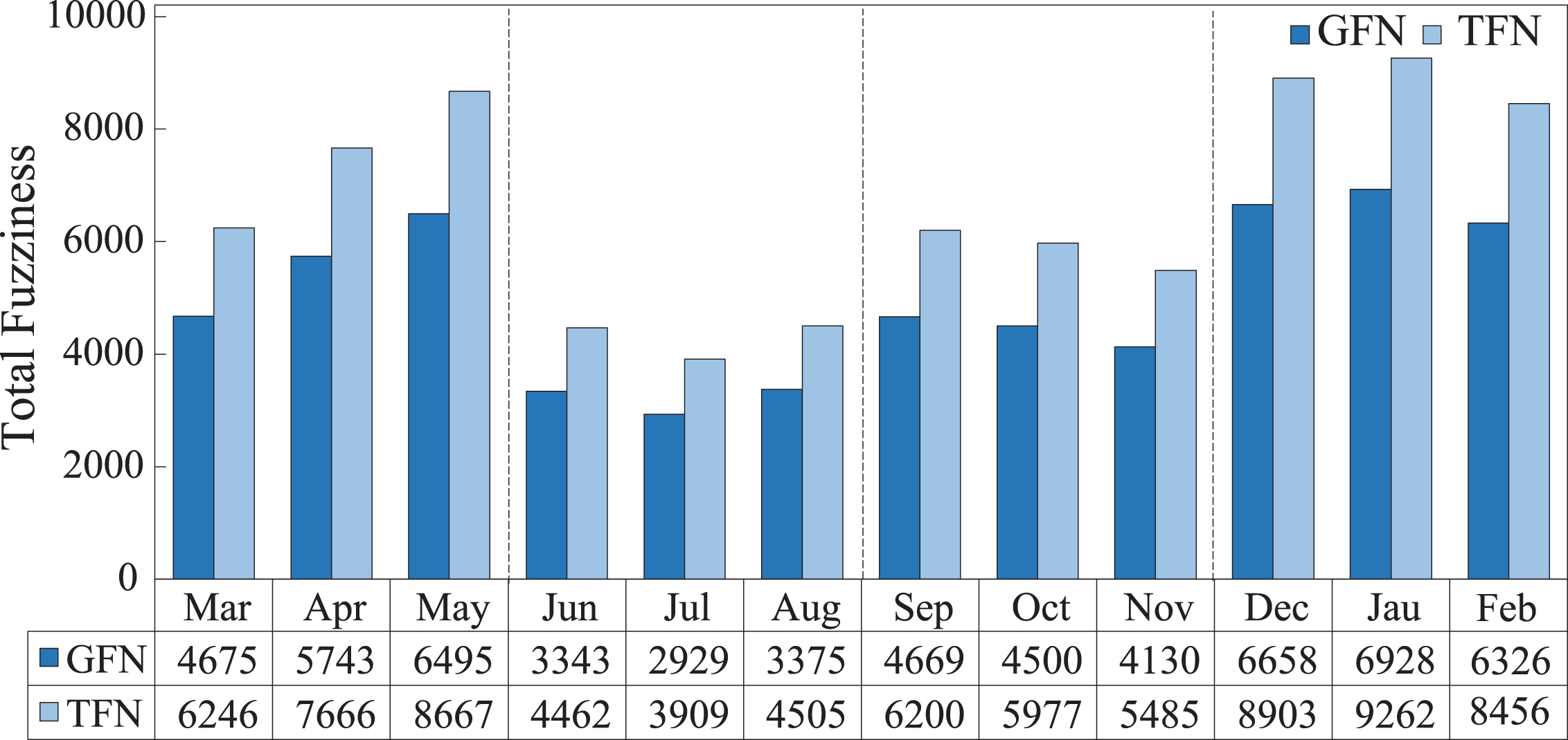
The monthly total fuzziness from March 2017 to February 2018.

The synthesis proposed by Figure 12 is further analyzed in graphical representations of the fuzziness obtained by the two classes of models for every single day in April 2017, as depicted in Figure 13. The vertical axis represents the date, whereas the horizontal axis represents the daily fuzziness with h = 0.8 on the left and h = 0.9 on the right, respectively. From the figure we can see, in each group, the light blue bar representing the daily fuzziness of the predicted AQI obtained by the TFN models is constantly longer than the dark blue one representing the result of the GFN models. In particular, the length of dark blue bars is up to almost twice as the light ones in the case of h = 0.9.

Fig. 13

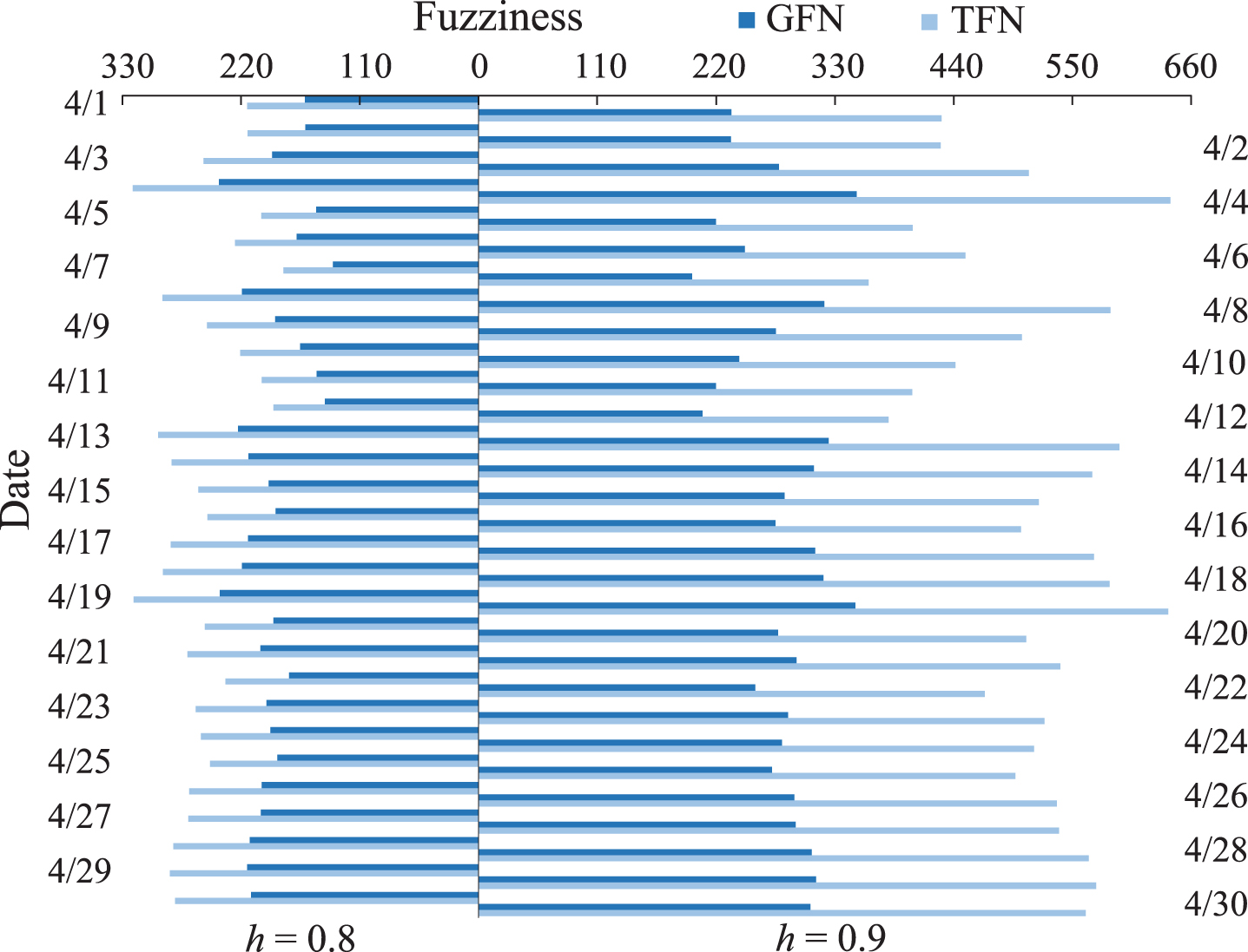
The daily fuzziness with h values at 0.8 and 0.9.

The monthly and daily data both reveals that the GFN models are far more practical with remarkable smaller fuzziness and therefore much higher determinacy of predicting the real value, while the membership degree of the real AQI is not considered.

C. Overall credibility

In addition to the membership degree and the fuzziness, the credibility is another crucial measure for validating the performance of the FLR models, and the comparative results based on this measure are more persuasive since it takes the two dimensions as a whole (see Figure 2 Part III for more details). Analogous to the other two measures, the monthly overall credibility of the predicted AQI from March 2017 to February 2018 is also figured out, by summing up the daily credibility (the ratio of the daily membership degree to the daily fuzziness) in each month. According to the results of the preceding two sections, it is readily to know that the overall credibility of the GFN models is higher than that of the TFN ones, just as Figure 14 shows, the bar in dark blue is longer than the one in light blue of the same month, and the seasonal overall credibility of the predicted AQI obtained by the GFN models are 36.31%, 27.38%, 24.65%, and 29.81% 6 , respectively, higher. In views of the statement in Section 2.4 that higher credibility is another way of saying higher reliability of the predicted AQI in representing the real one, the GFN models are enormously superior to the TFN models in terms of the credibility measure.

Fig. 14

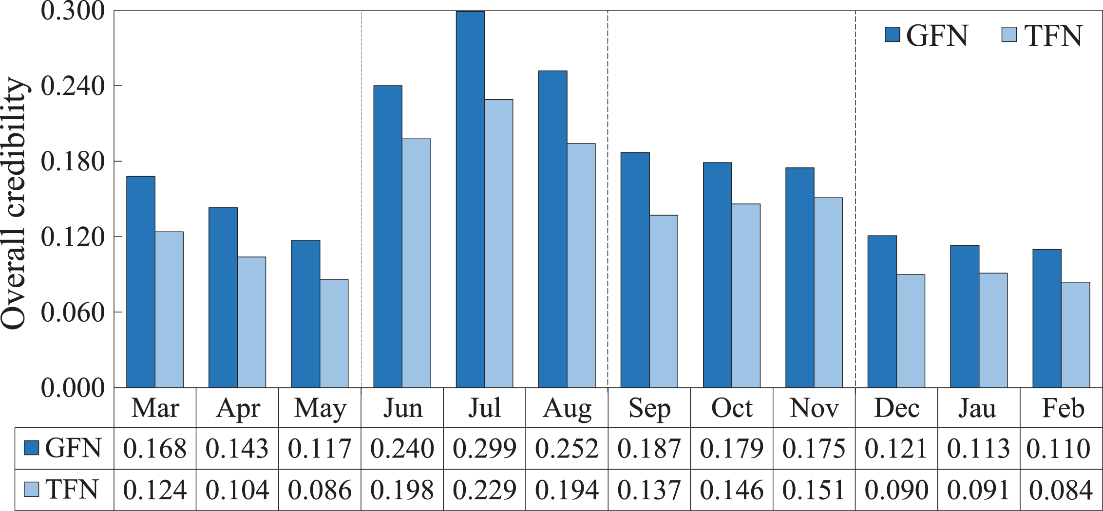
The monthly overall credibility from March 2017 to February 2018.

Similarly, by setting the h value as 0.8 and 0.9, respectively, we describe the daily credibility of the predicted AQI in April 2017 in Figure 15 to give an intuitive comparison detailedly. In the case of h = 0.8, the bars in dark blue (credibility derived from the GFN models) are slightly longer than the light blue ones (credibility derived from the TFN models) in the same day. Whereas when it comes to the case of h = 0.9, the differences are more visible. The results are consistent with the conclusions drawn by the daily fuzziness.

Fig. 15

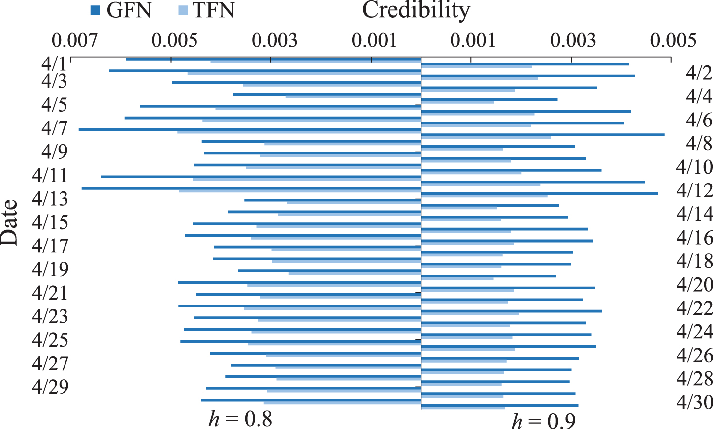
The daily credibility with h values at 0.8 and 0.9.

Overall, the information and the analyses totally indicate that the GFN models surpass the TFN ones so much in terms of membership degrees, fuzziness, and credibility. In other words, the validations demonstrate that the GFN models perform better with higher accuracy, determinacy as well as reliability. Thus, the FLR models with Gaussian fuzzy relationship between the meteorological factors and AQI are more reasonable and acceptable, at least on the present topic.

5 Conclusions

Considering the uncertainty of AQI and the meteorological factors in the atmospheric phenomena as well as the complicated relationships between them, this paper provided a new framework for AQI prediction from the perspective of fuzzy multiple linear regression as a kind of public service. The main work and conclusions of this paper can be summarised as follows:

(1) By summarizing the inherent correlation between the meteorological factors and the relationships between these factors and AQI, we observed that there were five imperative meteorological factors that is closely related to AQI. And the dependence relationship of AQI on the five factors can be expressed as an FLR model and converted into a linear programming using the minimum fuzziness criterion introduced by Tanaka [17] and the linearity of GFNs, which is consistent with the discovery of Wang et al. [16].

(2) Owing to its special geographic condition and significant seasonal characteristics concluded from the statistical analyses on data from March 2016 to February 2017, we found that it is reasonable to formulate the FLR models for Shanghai by season, and the fuzzy coefficients were well explained according to the climate characteristics of Shanghai. For example, atmospheric inversion often happens in Shanghai except for autumn, resulting in a positive relation between temperature and AQI in spring, summer and winter, and a negative relation in autumn. On the other hand, the unique distribution of the pollution sources in the city and its surrounding provinces as well as the changeable wind direction make a negative relationship between wind speed and AQI in spring and winter, whereas a positive one in summer and autumn. Furthermore, the results of the prediction via the data from March 2017 to February 2018, represented by the membership degrees in Figure 6 and the figures in Appendix 5, demonstrated that the FLR models based on GFNs is competent to describe the complicate relationships between the meteorological factors and AQI in the problem studied. For instance, the daily average membership degree in summer 2017 is 0.92, which is much larger than the predicted h value of 0.8 and very close to the maximum value of 1, indicating the high accuracy of the model regardless of the fuzziness.

(3) Concerning that TFN is more prevalent in the filed of fuzzy studies, we conducted some comparisons between the models based on GFNs and TFNs on the basis of the data from March 2017 to February 2018. The results demonstrated that GFNs are more appropriate than TFNs in representing the fuzzy relationships between the meteorological factors and AQI with higher membership degree, smaller fuzziness, and higher credibility. For instance, the seasonal cumulative membership degrees/total fuzziness/overall credibility of winter 2017 derived from the GFN models is 3.10% /25.20% /37.83% higher/lower/higher than the results of the TFN models. Overall, the results derived from the FLR models based on GFNs are more accurate, determined, and reliable, and the GFN models are more applicable in practice for AQI prediction.

Again, it should be noted that in the proposed approach, the fuzzy AQI was predicted by the meteorological factors of that very day, and in practice the values of these factors can be effectively predicted by the meteorological forecast center, therefore the FLR model is capable of predicting the AQI of the next few days so as to guide decisions making and support public traveling. In the future, a more practical and perfect system for the meteorological factors could be built through more sufficient practical research, and then the prediction performance of the model can be better.

Footnotes

Acknowledgments

This research was funded by the National Natural Science Foundation of China grant number 71872110 and the Funding of Innovation Team of Philosophy and Social Sciences of Henan Polytechnic University with the grant number CXTD2021-2.

Appendix

As shown in , the monthly cumulative membership degrees are recorded and classified into four groups by season. Accordingly, the percentage for each season is the ratio of the seasonal cumulative membership degrees derived from the GFN model to that of the TFN model minus 100%.

As shown in , the monthly total fuzziness is recorded and classified into four groups by season. Accordingly, the percentage for each season is the difference between 100% and the ratio of the seasonal total fuzziness derived from the GFN model to that of the TFN model. lower than that of the TFN models.

Based on the monthly overall credibility recorded in , the seasonal overall credibility are deduced, and the percentage for each season is the difference between the ratio of the seasonal overall credibility derived from the GFN model to that of the TFN model and 100%.

References

Kumar

and Goyal

, Forecasting of daily air quality index in Delhi, Sci Total Environ 409 (2011a), 5517–5523.

Kumar

and Goyal

, Forecasting of air quality in Delhi using principal component regression technique, Atmos Pollut Res 2 (2011b), 436–444.

Kumar

and Goyal

, Forecasting of air quality index in Delhi using neural network based on principle component analysis, Pure Appl Geophys 170 (2013), 711–722.

Liu

, Binaykia

, Chang

, Tiwari

M.K.

and Tsao

C.C.

, Urban air quality forecasting based on multidimensional collaborative Support Vector Regression (SVR): A case study of Beijing-Tianjin-Shijiazhuang, PloS One 12 (2017), e0179763.

Zhu

, Yang

, Wang

, Liu

, Lu

and Shen

, Optimalcombined model for air quality index forecasting: 5 cities in North China, Environ Pollut 243 (2018), 842–850.

, Wang

, Li

and Lu

, Novel analysis-forecast system based on multi-objective optimization for air quality index, J Clean Prod 208 (2019), 1365–1383.

Jiang

, He

and Tian

, A clustering-based ensemble approach with improved pigeon-inspired optimization and extreme learning machine for air quality prediction, Appl Soft Comput 85 (2019), 105827.

and Lin

, Daily urban air quality index forecasting based on variational mode decomposition, sample entropy and LSTM neural network, Sustain Cities Soc 50 (2019), UNSP 101657.

Chen

, Lu

, Li

and Wang

, Impact of fine particulate fluctuation and other variables on Beijing’s air quality index, Environ Sci Pollut R 22 (2015), 5139–5151.

10.

, Zhong

, Wang

, Yang

, Yao

and Huang

, Mapping comparison and meteorological correlation analysis of the air quality index in mid-eastern China, ISPRS Int J Geo-Inf 6 (2017), 52.

11.

Zadeh

L.A.

, Fuzzy sets, Inf Control 8 (1965), 338–353.

12.

Sarkheil

and Rahbari

, Development of case historical logical air quality indices via fuzzy mathematics (Mamdani and Takagi-Sugeno systems), a case study for Shahre Rey Town, Environ Earth Sci 75 (2016), 1319.

13.

Wang

, Li

and Lu

, Application of a novel early warning system based on fuzzy time series in urban air quality forecasting in China, Appl Soft Comput 71 (2018), 783–799.

14.

Liu

and Gao

, A new study on air quality sandards: Air quality measurement and evaluation for Jiangsu province based on six major air pollutants, Sustainability 10 (2018), 3561.

15.

Lin

, Zhao

, Li

and Sun

, Air quality forecasting based on cloud model granulation, EURASIP J Wirel Comm 2018 (2018), 106.

16.

Wang

, Zhao

, Han

and Zhou

, A fuzzy expression way for air quality index with more comprehensive information, Sustainability 9 (2017), 83.

17.

Tanaka

, Uejima

and Asai

, Linear regression analysis with fuzzy model, IEEE T Syst Man Cy 12 (1982), 903–907.

18.

Zhang

, Liu

and Zhao

, Singular value decomposition analysis of spatial relationships between monthly weather and air pollution index in China, Stoch Env Res Risk A 32 (2018), 733–748.

19.

Chen

, Chen

, Tang

and Wu

, Analysis of effect of me-teorological factor on air quality of Wuhan in -, Envi-ron Sci Technol 36 (2013), 130–133.

20.

Wyer

S.S.

, A treatise on producer-gas and gas-producers; Hill Publishing Company, New York, USA, 1907.

21.

, Xu

, Hong

, Chen

, Qiu

, Hu

, et al., The air pollution governed by subtropical high in a coastal city in South-east China: Formation processes and influencing mechanisms, Sci Total Environ 692 (2019), 1135–1145.

22.

Lee

J.Y.

, Jo

W.K.

and Chun

H.H.

, Characteristics of atmospheric visibility and its relationship with air pollution in Korea, J Environ Qual 43 (2014), 1519–1526.

23.

Luo

, Teng

, Yang

, Zhu

, Zhou

, Zhang

, et al., Research on PM2:5 estimation and prediction method and changing characteristics analysis under long temporal and large spatial scale - A case study in China typical regions, Sci Total Environ 696 (2019), UNSP 133983.

24.

Coppi

, D’Urso

, Giordani

and Santoro

, Least squares estimation of a linear regression model with LR fuzzy response, Comput Stat Data An 51 (2006), 267–286.

25.

Tanaka

, Fuzzy data analysis by possibilistic linear models, Fuzzy Sets Syst 24 (1987), 363–375.

26.

Tanaka

and Watada

, Possibilistic linear systems and their application to the linear regression model, Fuzzy Sets Syst 27 (1988), 275–289.

27.

Celminš

, Least squares model fitting to fuzzy vector data, Fuzzy Sets Syst 22 (1987), 245–269.

28.

Celminš

, Multidimensional least-squares model fitting of fuzzy models, Math Model 9 (1987), 669–690.

29.

Diamond

, Fuzzy least squares, Inform Sciences 46 (1988), 141–157.

30.

Wang

and Tsaur

R.C.

, Resolution of fuzzy regression model, Euro J Oper Res 126 (2000), 637–650.

31.

Mousavi

S.J.

, Ponnambalam

and Karray

, Inferring operating rules for reservoir operations using fuzzy regression and ANFIS, Fuzzy Sets Syst 158 (2007), 1064–1082.

32.

Moskowitz

and Kim

, On assessing the} value in fuzzy linear regression, Fuzzy Sets Syst 58 (1993), 303–327.

33.

Liu

and Chen

, A systematic approach to optimizing} value for fuzzy linear regression with symmetric triangular fuzzy numbers, Math Probl Eng 2013 (2013), 210164.

34.

Liu

, Chen

, Zhou

and Zhong

, Fuzzy linear regression models for QFD using optimized} values, Eng Appl Artif Intel 39 (2015), 45–54.

35.

Chen

, Chen

, Zhou

and Liu

, Optimizing} value for fuzzy linear regression with asymmetric triangular fuzzy coefficients, Eng Appl Artif Intel 47 (2016), 16–24.

36.

Azadeh

, Ghaderi

S.F.

and Gitiforouz

, Estimating electricity demand function in residential sector by fuzzy regression, 2006 IEEE International Symposium on Industrial Electronics, Montreal, Canada, 1-7 (2006), 390–394.

37.

Lin

K.P.

, Pai

P.F.

, Lu

Y.M.

and Chang

P.T.

, Revenue forecasting using a least-squares support vector regression model in a fuzzy environment, Inform Sciences 220 (2013), 196–209.

38.

Sassi

, Garcia

R.R.

, Boville

B.A.

and Liu

, On temperature inversions and the mesospheric surf zone,D, J Geophys Res-Atmos 107 (2002), 19.

39.

Die

, Nie

, Fang

, Yang

, Gao

, Tian

, et al., Seasonal and spatial distributions of atmospheric polychlorinated naph-thalenes in Shanghai, China, Chemosphere 144 (2016), 2134–2141.

40.

, Wang

, Deng

, McNeill

V.F.

, Fankhauser

, Wang

, et al., Insights into the characteristics and sources of primary and secondary organic carbon: High time resolution observation in urban Shanghai, Environ Pollut 233 (2018), 1177–1187.

41.

Yan

, Wang

, Zhou

, Liang

, Yin

and Wang

, Dynamic thermal rating of overhead transmission lines based on GRAPES numerical weather forecast, J Inf Process Sys 15 (2019), 724–736.

42.

Popescu

and Giuclea

, A model of multiple linear regression, P Romanian Acad A 8 (2007), 137–144.

43.

Buckley

J.J.

, Fuzzy statistics: Regression and prediction, Soft Comput 9 (2005), 769–775.

44.

Khan

U.T.

and Valeo

, A new fuzzy linear regression approach for dissolved oxygen prediction, Hydrolog Sci J 60 (2015), 1096–1119.

A fuzzy multiple linear regression model based on meteorological factors for air quality index forecast

Abstract

Keywords

1 Introduction

2.1 Meteorological factors selection

Table 2 The information of the dependent and independent variables Variable Symbol Description Units y ˜ AQI Fuzzy air quality index x 1 T Average temperature °C x 2 RH Average relative humidity % x 3 WS Average wind speed Km/h x 4 V Average visibility Km x 5 SLP Mean sea level pressure hPa

3.1 Data collection

3.2 Basic statistical analysis

4.1 Model verification

Footnotes

Acknowledgments

Appendix

References