
Abstract
Considering that most studies have taken the investors’ preference for risk into account but ignored the investors’ preference for assets, in this paper, we combine the prospect theory and possibility theory to provide investors with a portfolio strategy that meets investors’ preference for assets. Firstly, a novel reference point is proposed to give investors a comprehensive impression of assets. Secondly, the prospect return rate of assets is quantified as trapezoidal fuzzy number, and its possibilistic mean value and variance are regarded as prospect return and risk and then used to define the fuzzy prospect value. This new definition is presented to denote the score of an asset in investors’ subjective cognition. And then, a prospect asset filtering frame is proposed to help investors select assets according to their preference. When assets are selected, another new definition called prospect consistency coefficient is proposed to measure the deviation of a portfolio strategy from investors’ preference. Some properties of the definition are presented by rigorous mathematical proof. Based on the definition and its properties, a possibilistic model is constructed, which can not only provide investors optimal strategies to make profit and reduce risk as much as possible, but also ensure that the deviation between the strategies and investors’ preference is tolerable. Finally, a numerical example is given to validate the proposed method, and the sensitivity analysis of parameters in prospect value function and prospect consistency constraint is conducted to help investors choose appropriate values according to their preferences. The results show that compared with the general M-V model, our model can not only better satisfy investors’ preference for assets, but also disperse risk effectively.
Keywords
Introduction
To help investors disperse risk and make rational investment to some extent, portfolio selection has drawn a great attention from lots of researchers for many years. One of the most famous portfolio selection models is the M-V model (mean-variance probabilistic model), which was originally proposed by Markowitz [1] in 1952 and then became the basis of modern portfolio selection theory. In the M-V model, the distribution of return on an asset is considered as a random variable, and the mean value and variance of the variable are used to represent the return and risk of the asset respectively. M-V model requires investors to provide a given level of risk as the constraint and then maximizes the expected return, or provide a given level of return as the constraint and then minimize the risk. Although the model can balance return and risk to a certain extent, it is rough for the complex financial markets. Thus, many researchers studied the model and made some improvements, including adding complex realistic constraints or adopting more appropriate risk measures.
In recent years, more and more researchers focused on other ways to deal with the uncertainty of financial market. The prevalent view is that there are not only probabilistic factors but also non-probabilistic factors in the market. Therefore, it is necessary to search for an effective way to cope with these non-probabilistic factors. The fuzzy theory proposed by Zadeh [2] is one of the most popular tools to deal with non-probabilistic uncertainty for many fields, such as water quality [3], risk analysis [4], renewable power sources [5] and battery energy storage system [6]. For its effectiveness, many researchers combined it with portfolio selection to construct fuzzy models.
Although the uncertainty of financial market is well dealt with, the problem of investors’ subjective uncertainty is still exists. Most of the portfolio selection models are based on the hypothesis that investors are completely rational and not affected by the historical data, which makes the expected utility theory popular. However, in real-life investment, the investors are always bounded rationality while facing the risk [5], which would make them choose a portfolio that differs from the optimal one. Thus, integrating the irrational behavior of investors into portfolio selection model could provide them with more practical and flexible investment strategies. Prospect theory developed by Kahneman and Tversky [7] has outstanding performance on the decision making problem with bounded rationality, and has been widely applied in multi-attribute decision-making fields [8–12]. Although some researchers combined prospect theory with portfolio selection [13, 14], the studies in this field are still comparatively insufficient.
In this paper, we aim to combine prospect theory with portfolio selection to provide investors with strategies that satisfy their preference for assets. The main works of this paper are as follows: To introduce the prospect theory and give investors a comprehensive impression of all assets, a novel reference point is proposed based on the joint possibility distribution of assets. A new kind of fuzzy prospect value is proposed to denote the relative value of an asset, which can describe the return rate of an asset under unit risk in investors’ subjective cognition. It is used to construct the prospect asset filtering frame to help investors select assets. To measure the consistency between an optimal strategy provided by portfolio selection model and the investors’ preference for the assets, we define the prospect consistency coefficient and then present some theorems and proofs. In order to ensure that the optimal strategy can satisfy investors’ preference for assets, a new model with prospect consistency constraint is constructed. The numerical example shows that compared with the general M-V model, our model can not only better satisfy investors’ preference for assets, but also disperse risk effectively.
The rest of this paper is organized as follows: In Section 2, we review some related works of portfolio selection. In Section 3, some basic definitions of possibility theory and prospect theory are introduced. Section 4 presents a novel reference point and the definition of fuzzy prospect value to construct the prospect asset filtering framework. In Section 5, the definition of prospect consistency coefficient and the possibilistic model with prospect consistency constraint are proposed. The numerical example is given in Section 6 and the sensitivity analysis is conducted in Section 7. Finally, the conclusion is given in Section 8.
Related work
Portfolio selection based on probability theory
Most of the portfolio selection models are developed from the M-V model proposed by Markowitz [1]. These models took the complex realities into account and then improved the model. For example, Chunhachinda et al. [15] pointed out that some major stock markets are not normally distributed and the incorporation of skewness into portfolio causes a major change in the construction of the optimal portfolio; Mansini and Speranza [16] dealt with the portfolio problem with minimum transaction lots and showed that the problem of finding a feasible solution is, independently of the risk function, NP-complete in this case; Maccheroni et al. [17] proposed a portfolio selection model based on a class of preferences, and they stressed that these preferences can only ensure consistency with mean-variance preferences in the monotonicity domain; Wang and Liu [18] investigated the multi-period mean-variance portfolio selection problems with fixed and proportional transaction costs; Masmoudi and Abdelaziz [19] studied the portfolio selection problem when the loss in the portfolio return is considered as a recourse cost. For this problem, they found that the investor would penalize unfeasible solutions for uncertain constraints with the most probable highest recourse cost rather than with the expected recourse cost as in the traditional recourse approach.
What these models have in common is that they are based on probability theory. However, the financial market is always too complex to predict the probabilistic distribution of assets. In addition, its uncertainty cannot be completely described by probabilistic factors. Thus, in this paper, we use another effective tool, i.e. fuzzy set, to deal with the complex uncertainty of financial market.
Portfolio selection based on fuzzy theory
The fuzzy theory proposed by Zadeh [2] provides an effective way to deal with non-probabilistic uncertainty for many fields, and has been widely used in portfolio selection. Based on the possibility theory proposed by Carlsson and Fullér [20], Chen et al. [21] presented a possibilistic mean VaR model for portfolio selection; Deng and Li [22] studied the portfolio selection problem with borrowing constraint; Zhang et al. [23] put forward a fuzzy programming approach for multi-period portfolio optimization with return demand and risk control; Zhou et al. [24] studied stock portfolio selection problem based on varying conservative-neutral-aggressive attitudes where the return rates of stocks are characterized by fuzzy variables; Li and Yi [25] developed a new trapezoidal fuzzy number with an adaptive index to capture the coherence of investor’s expectation; Zhang [26] thought that practical portfolio selection problems often involve the mixture of the stochastic returns with fuzzy information, so that he proposed a mean variance random credibilitic portfolio selection model with different convex transaction costs.
Some of these studies may take the investors’ preference for risk into account, thus they can offer investors more practical strategies. Nevertheless, for all we know, there are few studies that have considered the investors’ preference for assets. In fact, the investors’ preference for assets will affect their acceptance of the strategies provided by the model. In this respect, it is necessary to introduce the investors’ preference for assets into portfolio selection model, which is one of the highlights of our paper.
Decision-Making based on prospect theory
In portfolio selection, investors may choose investment strategy according to the returns and risks of assets. If we take the returns and risks of assets as two different criteria, it is no doubt that portfolio selection problem can be regarded as a kind of multi-criteria decision-making (MCDM) problem. Most MCDM problems have attached great importance to the psychological factors of decision makers. Yu et al. [27] proposed some new formulae to calculate the gain and loss for an unbalanced HFLTS over another, and then extended the classical TODIM method to deal with multi-criteria group decision making (MCGDM) problems with unbalanced HFLTSs by considering the psychological behavior of decision makers; Zhang et al. [28] presented an extended logarithmic least squares method to derive a priority weight vector from an fuzzy preference relation with self-confidence (FPR-SC), and then applied it to develop a novel approach to two-sided matching decision making with FPR-SC; Zhang et al. [29] defined two consensus measures to identify the leadership of experts and designed a new feedback mechanism to help experts reach consensus in group decision-making process.
Prospect theory, which developed by Kahneman and Tversky [7], focuses on people’s irrational decision-making psychology. It pointed out that people may be influenced by the relative values of alternatives in decision-making process. For its effectiveness, many studies have used prospect theory to solve MCDM problem. Lin et al. [30] set up a dynamic price recommendation method for housing purchases and applied the fuzzy multiple criteria decision making (FMCDM) technique based on the prospect theory of the loss aversion effect; According to the time degree and the prospect value deviation of alternatives in different periods, Dai et al. [31] constructed the triangular fuzzy prospect decision matrices to solve the multi-stage multi-attribute decision-making problem with completely unknown period weights and attribute weights; Tian et al. [32] developed an ULZN-based QUALIFLEX (qualitative flexible multiple criteria method) by considering the decision-maker’s psychological behavior character, and then utilized it to solve a qualitative MCDM problem with larger number of criteria than alternatives; Ma and Zhang [33] proposed a distance measure for normal cloud, set the positive ideal reference point based on prospect theory and then established an optimization model for handling incomplete attribute weights to obtain the ranking of alternatives.
Considering that most studies have taken the investors’ preference for risk into account [13, 14] but ignored the investors’ preference for assets, and the studies of portfolio selection based on prospect theory is insufficient, in this paper, we combine the prospect theory and possibility theory to provide investors with strategies that can meet their preference for assets. Firstly, a novel reference point is proposed to compare the assets with all the others and then provide investors with a comprehensive impression of these assets. Secondly, the prospect return rates of each asset are quantified by the subtraction of trapezoidal fuzzy number to obtain the prospect possibilistic mean values and variances as prospect returns and risks. Based on the prospect return and risk, a new definition called fuzzy prospect value is presented to denote the score of an asset in investors’ subjective cognition. And then, a prospect asset filtering frame is put forward to help investors select a certain number of assets from a large set, which can ensure that all the selected assets have the highest score to satisfy investors’ preference.
In order to provide investors with optimal strategies based on their preference for assets, another new definition called prospect consistency coefficient is proposed. The definition can measure the deviation of a portfolio strategy from investors’ preference with range [0, 1]. And then, a possibilistic model based on the definition is constructed. The model can not only provide investors with optimal strategies to make profit and reduce risk as much as possible, but also ensure that the deviation between the strategies and investors’ preference is tolerable. In addition, based on the Shannon entropy [34], it is proved that our model can effectively disperse risk compared with the general model.
Preliminaries
In this section, some definitions of possibility theory and prospect theory will be briefly mentioned for the following sections.
Possibility theory
A fuzzy number is formally interpreted as a normalized convex fuzzy set with its membership function being piece-wise continuous [25]. The membership function is used to represent the membership degree of the variable belonging to the fuzzy set. Generalized trapezoidal fuzzy number is one of the most typical fuzzy numbers, which is presented as follows:
If r2 = r3, R regresses to a generalized triangular fuzzy number; If r1 = r2 and r3 = r4, R regresses to an interval number; If r1 = r2 = r3 = r4, R regresses to a real number.
By formula (2), the possibilistic mean value of generalized trapezoidal fuzzy number R = (r1, r2, r3, r4) is
According to formula (4), the possibilistic variance of generalized trapezoidal fuzzy number R = (r1, r2, r3, r4) is
According to formula (6), the possibilistic covariance of generalized trapezoidal fuzzy numbers R1 = (r11, r12, r13, r14) and R2 = (r21, r22, r23, r24) is
From these definitions, it is not difficult to find that possibilistic mean value, possibilistic variance and possibilistic covariance have the following properties, which are similar to the properties of mean, variance and covariance in probability theory.
Obviously, A - B is still a trapezoidal fuzzy number.
As an effective tool to deal with the decision makers’ bounded rationality in decision making process, prospect theory points out that people would make a decision based on the prospect value rather than the expected utility. Unlike expected utility, prospect value depends on reference point and the relative gains or losses but not the absolute outcomes. The prospect value function presented by Tversky and Kahneman [7] is given as follows:
Where Δx i denotes the gain or loss from event a i relative to the reference point, α and β respectively represent the decision makers’ sensitive degree on gain and loss, λ is the parameter to reflect the decision makers’ risk aversion degree. Generally, we have 0 < α < 1 and 0 < β < 1, which explain the phenomenon called sensitivity decline; In addition, the value of λ is higher than 1, which implies that decision makers are always loss averse. According to Tversky and Kahneman’s empirical research [36], the values of these parameters could be taken as α = β = 0.88, λ = 2.25.
Tversky and Kahneman also stressed that people often distort objective probability. That is, people would overestimate lower probability and underestimate higher probability. Thus, they proposed the probability weighting function to describe this phenomenon:
In the formula, p i (p i ⩾ 0) is the objective probability of event a i , γ and δ represent the decision makers’ attitude coefficients toward the relative gain and loss, respectively. The values of γ and δ denote the distortion degrees of the original probability. The smaller the values are, the severer the distortion. The values given by Tversky and Kahneman [36] are γ = 0.61, δ = 0.69.
Based on the formulas (11) and (12), if there are n possible events a1, a2, ⋯ , a
n
generated by decision x, and p
i
(p
i
⩾ 0) is the objective probability of action a
i
,
In prospect theory, it is important to select a reference point for it could make a great influence on the final decision. Usually, the reference point should be decided at first for the calculation of relative gains or losses. However, a different problem should be solved before deciding the reference point.
The problem is raised based on the premise that the return rates of assets are regarded as generalized trapezoidal fuzzy numbers. Hence, it requires us to find a proper way to transform formula (13) into the form that is suitable for fuzzy numbers. In fact, some researchers have combined prospect theory with fuzzy numbers [5, 37]. Let’s compare their methods and select the better one for portfolio selection.
Let R = (r1, r2, r3, r4) be a trapezoidal fuzzy number, its prospect value function is:
V (R) = (- λ (- r1)
β
, - λ (- r2)
β
, - λ (- r3)
β
, -λ (- r4)
β
), if r1 ⩽ 0, r2 ⩽ 0, r3 ⩽ 0, r4 ⩽ 0;
V (R) = (- λ (- r1)
β
, - λ (- r2)
β
, - λ (- r3)
β
,
Where parameters α, β and λ are the same as in the formula (11).
In this paper, Method II would be used and extended for portfolio selection with the reasons listed as follows: It is obvious that the prospect value function in Method II is based on the formula (11), and it is still a trapezoidal fuzzy number that could better reflect the uncertainty of the original. Method I strongly depends on the predetermined distance measure of fuzzy numbers. Considering that there are many distance measures for trapezoidal fuzzy number [4, 39], it is difficult for investors to find the appropriate one. Comparatively, the subtraction of trapezoidal fuzzy number is unique and has the rigorous theoretical basis [35]. Therefore, if the reference point (also in the form of trapezoidal fuzzy number) is determined, the relative gain or loss could be obtained uniquely by the subtraction and then the prospect value function could be identified according to Method II. Suppose the distance measure is predetermined in Method I, and there is only one criterion, the return rate, to select some assets for portfolio. In this case, the weight of the return rate is 1, which means the prospect weight will also be 1 and Step 4 will be meaningless. Even if investors may choose more than one criterion to select assets for portfolio, it is doubtless that the weight allocation method (such as AHP, BWM and entropy weight method [40–42]) for each criterion could make a great influence on the result. For investors, it is also a thorny problem to choose an appropriate method to allocate weight for criteria.
In summary, although Method I is effective for MCDM problem, it is unsuitable for portfolio selection problem. Therefore, Method II would be used in this paper. Considering Method II only provides us with the form of prospect value function, in the following sections, we would extend Method II based on the subtraction of trapezoidal fuzzy number and possibility theory.
A novel prospect asset filtering frame for portfolio selection
A novel reference point for comprehensive comparison
As mentioned above, the selection of reference point is important in prospect theory. Many kinds of reference points had been used in some existing studies, such as average, medium point, zero point, optimal point and worst point [8, 43]. In this paper, a novel kind of reference points is put forward.
Firstly, it should be pointed out that the method we use to quantify the return rates of assets as trapezoidal fuzzy numbers is proposed by Vercher and Bermudez [44]. That is, the weekly turns will be transformed into the form of (r10, r40, r60, r90), where r q is the qth sample percentile of historical returns.
On this basis, if there are n assets A1, A2, ⋯ , A
n
with the return rates R1, R2, ⋯ , R
n
in the form of trapezoidal fuzzy number, let S be the set of the historical returns of all the assets, the novel reference point RF is given in the following form:
The feature of the proposed reference point is: if we use the trapezoidal fuzzy number (ri,10, ri,40, ri,60, ri,90) to quantify the return rate of asset A i , that is, the possibility distribution of R i is assumed as a trapezoidal fuzzy number, then, RF can be regarded as the possibility distribution of S, which is equivalent to the joint possibility distribution of R1, R2, ⋯ , R n .
Thus, using RF as a reference point indicates that each asset will be compared with all other assets, which meets investors’ demands and makes the result more comprehensive.
Based on the proposed reference point, the relative gains or losses of each asset can be easily obtained by the subtraction of trapezoidal fuzzy number according to Definition 5.
For the assets A1, A2, ⋯ , A
n
with the return rates R1, R2, ⋯ , R
n
in the form of trapezoidal fuzzy number, the relative gain or loss of asset A
i
is:
Then, by Method II, we can get the prospect return rate V (R i - RF) for asset A i . According to Definitions 2 and 3, the possibilistic mean value and variance of V (R i - RF) can also be calculated.
It is common that an investor would collect the historical returns of many assets and then choose some assets for investment. In this part, a prospect asset filtering framework is proposed to help investors select assets. For convenience, suppose there are n assets A1, A2, ⋯ , A n with the return rates R1, R2, ⋯ , R n , R i = (r1i, r2i, r3i, r4i). If the investor wants to choose m of them to invest in (m ⩽ n), the following operations would be taken:
The prospect asset filtering framework can be briefly summarized in the following steps:
Figure 1 shows the process of asset filtering.

The process of asset filtering.
The prospect inconsistency coefficient and prospect consistency coefficient
Since we cannot ensure that a selected asset will make profit, it is necessary to invest in multiple assets at the same time to disperse risk. However, how to allocate the investment ratio to each asset is also a problem. As mentioned in introduction, many researchers have studied the problem, but most of them assumed that investors are completely rational and strongly depend on the expected utility theory. In fact, investors would be affected by the historical returns of assets and the comparison between assets. On the one hand, they would have an impression of each asset when they collect the historical data, which would have a great influence on their final decision. On the other hand, they want to make profit and reduce risk as far as possible. For this phenomenon, a new definition called prospect inconsistency coefficient is proposed.
Firstly, in Section 4, the relative fuzzy prospect values of each remaining asset are obtained. These values could be viewed as the scores of each asset in investors’ subjective cognition, which are the quantification of the impressions of each asset. In general, investors would like to allocate more investment to the assets with higher scores. For instance, if there are two assets A and B with the return rates shown in Table 1, investors will allocate more investment ratio to A rather than to B. Especially, investors would like to allocate 75% investment ratio to A and 25% investment ratio to B because A gains three times as many scores as B in investors’ subjective cognition.
The return rates of assets A and B
The return rates of assets A and B
It is common that people often distribute their property simply according to the value ratio of things. For example, with the same price, if a concert can bring audiences two times the joy of a football match, people may go to concerts twice a week, but only watch football match once a week. Similarly, we can use the ratio of relative fuzzy prospect value to describe the investors’ preference for assets.
Suppose the relative fuzzy prospect values of the top m selected assets A1, A2, ⋯ , A
m
are RFV1, RFV2, ⋯ , RFV
m
, RFV
i
⩾ 0, i = 1, 2, ⋯ , m. Considering that it is almost impossible for an asset’s historical data to be exactly the same as others, and the number of remaining assets is more than m, we can assume that RFV
i
> 0, i = 1, 2, ⋯ , m (Otherwise, exclude the assets with RFV
i
= 0 and then repeat Step 5 of the prospect asset filtering frame until the condition is satisfied). Then, the prospect investment ratio
It is easy to prove that the formula can be satisfied at the same time for all
However, investors do not simply allocate investment ratios based on the scores of each asset. They will choose a good portfolio strategy to make great profit while reducing risk as much as possible, if the actual investment ratios do not deviate too much from the prospect investment ratios (or they would not feel well and dismiss the portfolio strategy). The prospect inconsistency coefficient is defined to quantify the deviation between the actual investment ratios and the prospect investment ratios.
It is easy to find that PIC i (X) ⩾0 (i = 1, 2, ⋯ , m), thus, PIC (X) ⩾ 0.
For any number 0⩽ A < + ∞, if PIC (X) = A, then we have
For any number A > 0, let
In addition,
If
Since
In conclusion, the range of PIC (X) is [0, + ∞).
Now let us turn back to the definition of prospect inconsistency coefficient. Considering the case that investors could only select one asset to invest in. If the prospect inconsistency coefficient is defined as
Since the range of PIC (X) is [0, + ∞), which cannot provide investors with an intuitive appreciation, the definition of prospect consistency coefficient is presented as follows.
The relationship between PIC (X) and PCC (X) is similar to that between similarity measure and distance measure [4].
According to Theorems 1 to 3, we have
Prospect consistency coefficient can describe the consistency between a portfolio strategy and investors’ preference with range [0, 1]. In the next part, we will construct a portfolio selection model with prospect consistency constraint to provide investors with a satisfactory portfolio strategy while making profit and reducing risk as much as possible.
Based on possibility theory, we can get the expected return and risk of a portfolio strategy by possibilistic mean value and variance. Many researchers constructed models to maximize possibilistic mean value while minimizing possibilistic variance to get an optimal portfolio strategy. However, as mentioned above, if a portfolio strategy strongly deviates from investors’ preference, it would not be adopted because it conflicts with investors’ intuition and cannot gain their trust. For this reason, a possibilistic portfolio model with prospect consistency constraint is proposed. The model takes the prospect consistency coefficient as constraint to reflect investors’ tolerance level of the deviation between the portfolio strategy and their preference. And then, within investors’ tolerance level, the model would provide them with an optimal strategy.
The model is constructed as follows.
Where X = [x1, x2, ⋯ , x
n
]
T
is the portfolio strategy, x
i
is the investment ratio of A
i
, R
i
= (r1i, r2i, r3i, r4i) is the return rate of A
i
in trapezoidal fuzzy number form,
According to Theorem 6, the range of parameter δ is [0, 1]. It is apparent that the greater the value of δ, the lower the investors’ tolerance level. When δ = 0, the prospect consistency constraint is meaningless, and Model (26) regresses to the general possibilistic M-V model.
By Properties 1 and 2, the formulas (3) and (7), and the definition of PCC (X), Model (26) can be rewritten as
Where RFV i is the relative fuzzy prospect value of A i .
Considering that there are too many constraints PIC
i
(X) of the model, which would make the model over-complicated and inflexible, it is better to simplify the model. Similar to the BWM method and AHP method [40, 41], in reality, investors will not compare all the assets in pairs. They prefer to select the best one and the worst one, and then compare each asset with these two assets. Therefore, denote RFV
best
and RFV
worst
as the maximum and minimum relative fuzzy prospect values, respectively, and then let x
best
, x
worst
be the investment ratios allocated to the assets with RFV
best
and RFV
worst
. Model (27) can be simplified as follows.
Notice that there is a new constraint x worst ⩽ x i ⩽ x best in Model (28). This constraint satisfies investors’ preference according to formula (19) and will make the portfolio strategy more acceptable.
To solve the proposed model, let
In addition, it is easy to find that the range of these new objective functions is [0, 1]. It can be considered that the new objective functions represent the degrees that the original objective functions reached when X ∈ D. The ideal strategy is to make the degrees reach 1. However, it is impossible because of the conflict between risk and return, so that it is necessary to balance the new objective functions. In this paper, the method to balance the objectives is to transform Model (28) into the following single objective model:
We can ensure that the feasible region of Model (31) is not empty. In fact, let
For convenience, if we denote
Asset filtering process
In order to verify the validity of the proposed model, in this section, a numerical example is provided.
Suppose there are 10 assets A1, A2, ⋯ , A10 for portfolio selection and an investor wants to choose six of them for investment. To make the example more realistic, the weekly returns of some securities are used, including FTSE 100 Index, DAX 30 Index, CAC 40 Index, AEX Index, BEL 20 Index, SMI Index, PSI 20 Index, S&P 500 Index, KLCI (KLSE) Index and Nikkei 225 Index. All the historical data are from January 4, 2008 to July 26, 2019, and the method to quantify the return rates of assets as trapezoidal fuzzy number is proposed by Vercher and Bermudez [44]. Then, the return rates are listed in Table 2.
The return rates of assets A1, A2, ⋯ , A10
The return rates of assets A1, A2, ⋯ , A10
According to Section 4.1, the reference point is also quantified and shown in Table 2. Next, we will use the prospect asset filtering frame to filter these assets.
According to formulas (15) and (17), the prospect return rates of each asset are calculated and listed in Table 3. Here, the values of parameters α, β and λ are taken as α = β = 0.88 and λ = 2.25, which is given by Tversky and Kahneman [36].
The prospect return rates of assets A1, A2, ⋯ , A10
According to formulas (3), (5), (16) and (18), the prospect possibilistic mean values
The ranking of assets based on the relative fuzzy prospect values is also shown in Table 4. From Table 4, we know that DAX 30 Index, CAC 40 Index, AEX Index, BEL 20 Index, S&P 500 Index and Nikkei 225 Index will be selected to invest in. In addition, we can find that A2 is the asset with the maximum relative fuzzy prospect value and A8 is the selected asset with the minimum relative fuzzy prospect value.
Suppose the investor’s tolerance level is 0.2, that is, δ = 0.8. To make profit and reduce risk as much as possible, a portfolio selection model is constructed based on Model (31) as follows.
Where X = [x1, x2, x3, x4, x5, x6]
T
are the investment ratios of assets A2, A3, A4, A5, A8, A10, X
T
is the transpose of X and C is the covariance matrix of these assets,
For comparison, the possibilistic M-V model is also constructed as follows.
Model (34) will be transformed into a single objective model in the same way as Model (28). And then, we input the data into Lingo software to obtain the optimal solutions of these two models, which are shown in Table 5.
The optimal solutions of Models (32) and (34)
Based on Table 5, the returns (mean), risks (variance), Shannon entropy [34], the values of the objective θ and the prospect consistency coefficient
The returns, risks, Shannon entropy, θ and PCC of Models (32) and (34)
The concept of entropy was originally derived from thermo-dynamics to describe the disorder of a system. Later, for its ability to measure diversity, it is widely used in many fields including portfolio selection. The formula of Shannon entropy is given as follows.
The greater the entropy is, the higher the diversity. The higher the diversity is, the greater the risk dispersion.
From Table 6, we can find that: The return and risk of the optimal strategy obtained by our proposed model are worse than that of the general model. Similarly, the value of objective θ, the degree that the original objective functions ( The Shannon entropy of the proposed model is far higher than that of the general. In fact, from Table 5, we can see that the portfolio strategy obtained by our model is more diverse. Comparatively, the portfolio strategy obtained by the general model only allocates the investment ratios to two assets, which shows the poor ability to disperse risk. Although A2 is the asset with the maximum relative fuzzy prospect value, from Table 5, we can see that the general model does not allocate any investment ratio to A2, which is inconsistent with the investor’s preference and then leads to a small value of PCC.
In summary, compared with the general model, our model can provide investors with a more satisfactory portfolio strategy and better disperse risk.
In this section, the sensitivity of parameters α, β and λ in formula (11) and parameter δ in Model (31) will be analyzed to study their properties and then help investors choose appropriate values according to their preferences. For convenience, the data used in Section 6 will also be used in the following.
The sensitivity analysis of parameters α, β and λ
Considering the values of α and β are the same (0.88) based on Tversky and Kahneman’s empirical research [36], in this part, we will keep α = β in all times. And then, changing the value of α from 0.1 to 0.9 while changing the value of λ from 1.1 to 2.9. The results are shown in Tables 7 9 and Figs. 3 5.
The returns of Model (31) with δ = 0.8 and α = β
The returns of Model (31) with δ = 0.8 and α = β
The risks of Model (31) with δ = 0.8 and α = β
The Shannon entropy of Model (31) with δ = 0.8 and α = β

The asset selection distribution.
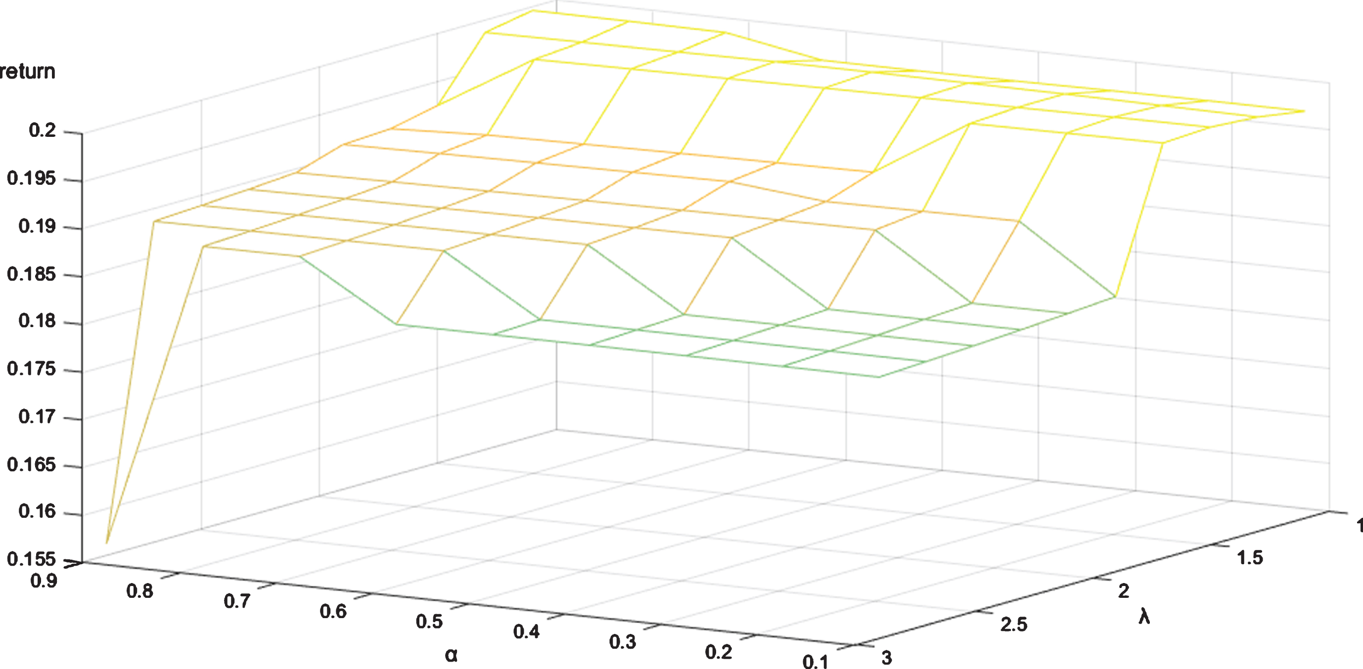
The returns of Model (31) with δ = 0.8 and α = β.
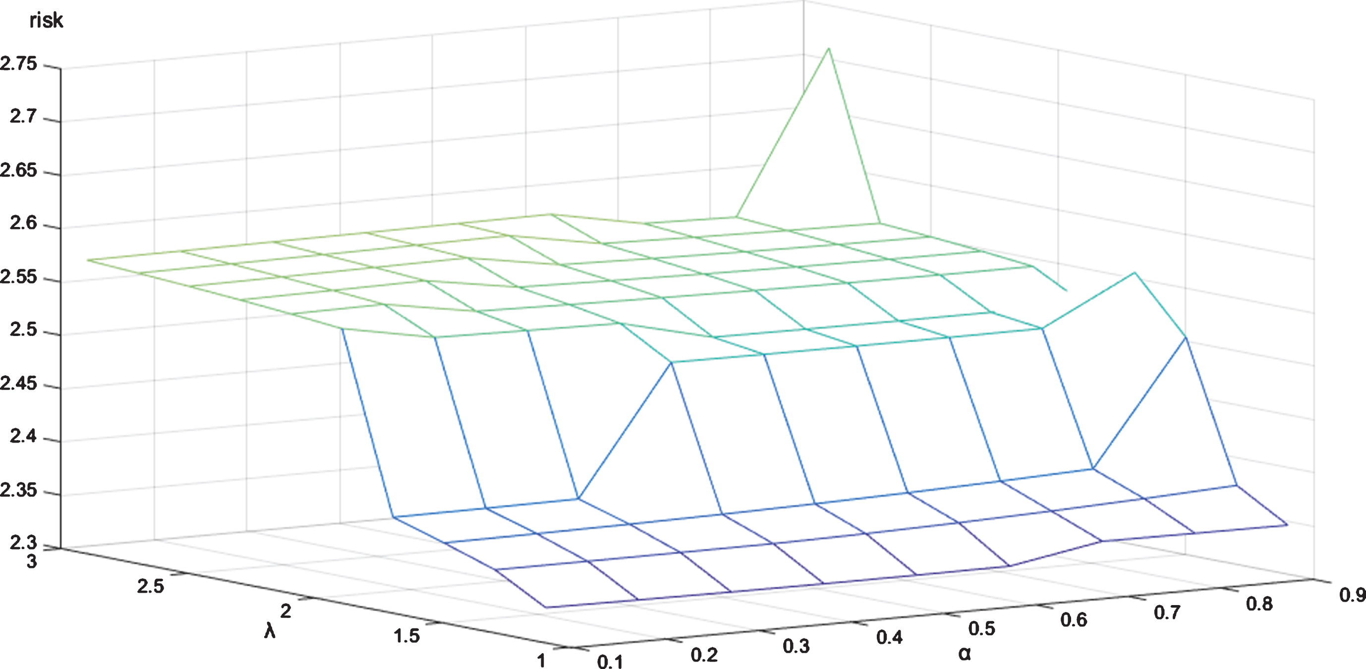
The risks of Model (31) with δ = 0.8 and α = β.
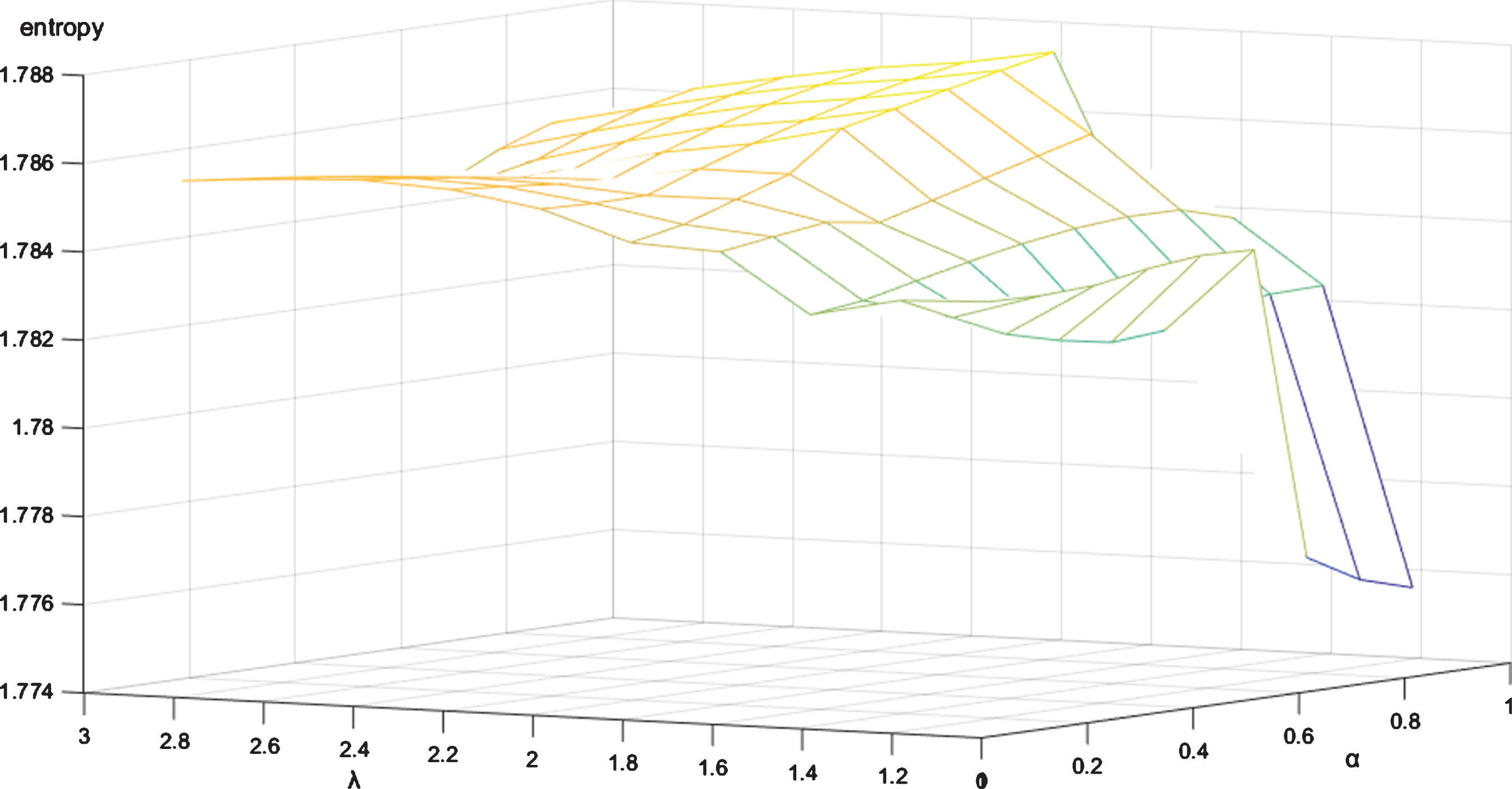
The Shannon entropy of Model (31) with δ = 0.8 and α = β.
It should be noticed that when the values of α, β and λ are changed, the prospect return rates of each asset are also changed. In other words, the prospect possibilistic mean values, prospect possibilistic variances, fuzzy prospect values and relative fuzzy prospect values are all changed so that the ranking of assets is changed and the assets selected to invest in would be different. The asset selection distribution is shown in Fig. 2.
From Fig. 2, we can find that: In all the cases, the investment ratios of assets A1, A9 are all zero, which indicates that neither of these two assets has ever been selected to invest in. A7 is similar to them. In fact, A7 is selected only once when α, β = 0.9 and λ = 2.9, which is the reason that return decreases sharply and risk increases sharply in that case (see Figs. 3 and 4). In all the cases, the investment ratios of assets A2, A3, A4, A8, A10 are higher than 0.1, which indicates that these assets have a good performance and are not affected by the parameters. In addition, we can find that the investment ratio of A2 is the highest at all times. According to the constraint x
worst
⩽ x
i
⩽ x
best
(i = 1, 2, ⋯ , n) of Model (31), it can be inferred that A2 is the asset with the maximum relative fuzzy prospect value no matter how the parameters change. Based on (i) and (ii), it is not difficult to find that either A5 or A6 is the last selected asset in most cases. The minimum investment ratio allocated to these two assets is zero, which means that sometimes they are not selected. In fact, when A5 is selected, A6 is excluded; when A6 is selected, A5 is excluded.
From Tables 7 9 and Figs. 3 5, we can find that: In most cases, the return obtained by the proposed method increases if λ decreases. Comparatively, the sensitivity of return to parameters α and β is far less than that to λ. In addition, when 0.1 ⩽ α, β ⩽ 0.3, there is a sharp decrease of return from λ = 1.7 to λ = 1.9; when 0.3 ⩽ α, β ⩽ 0.8, there is a sharp decrease of return from λ = 1.5 to λ = 1.7; when α, β = 0.9, there is a sharp decrease of return from λ = 1.3 to λ = 1.5. That is, the sharp decreasing point λ0 decreases when α and β increase. In most cases, the risk obtained by the proposed method increases if λ increases. Comparatively, the sensitivity of risk to parameters α and β is far less than that to λ. In addition, when 0.1 ⩽ α, β ⩽ 0.3, there is a sharp increase of risk from λ = 1.7 to λ = 1.9; when 0.3 ⩽ α, β ⩽ 0.8, there is a sharp increase of risk from λ = 1.5 to λ = 1.7; when α, β = 0.9, there is a sharp increase of risk from λ = 1.3 to λ = 1.5. That is, the sharp increasing point λ0 decreases when α and β increase, which is similar to (i). In most cases, when λ ⩾ 1.9 and The values of Shannon entropy are more than 1.774 in all the cases, which is far higher than that of the general model in Section 6. It shows that our model can better help investors disperse risk no matter how the parameters change.
In conclusion, assets A2, A3, A4, A8, A10 are worth selecting and A5, A6 can be selected according to investors’ preference. And then, with a sufficient risk dispersion, investors can decide the values of parameters α, β and λ according to their risk preference. If investors are risk averse, the values of these parameters should be small; Otherwise, investors can choose a small value for λ and a large value for α, β.
In this part, the parameter δ in Model (32) is changed from 0 to 1 to analyze the relationship between optimal portfolio strategy and the investors’ preference for assets. The results are shown in Tables 10 11 and Figs. 6 7.
The optimal portfolio strategy of Model (32) with α = β = 0.88 and λ = 2.25
The optimal portfolio strategy of Model (32) with α = β = 0.88 and λ = 2.25
The return, risk, Shannon entropy, θ and PCC of Model (32)

The optimal portfolio strategy of Model (32) with α = β = 0.88 and λ = 2.25.
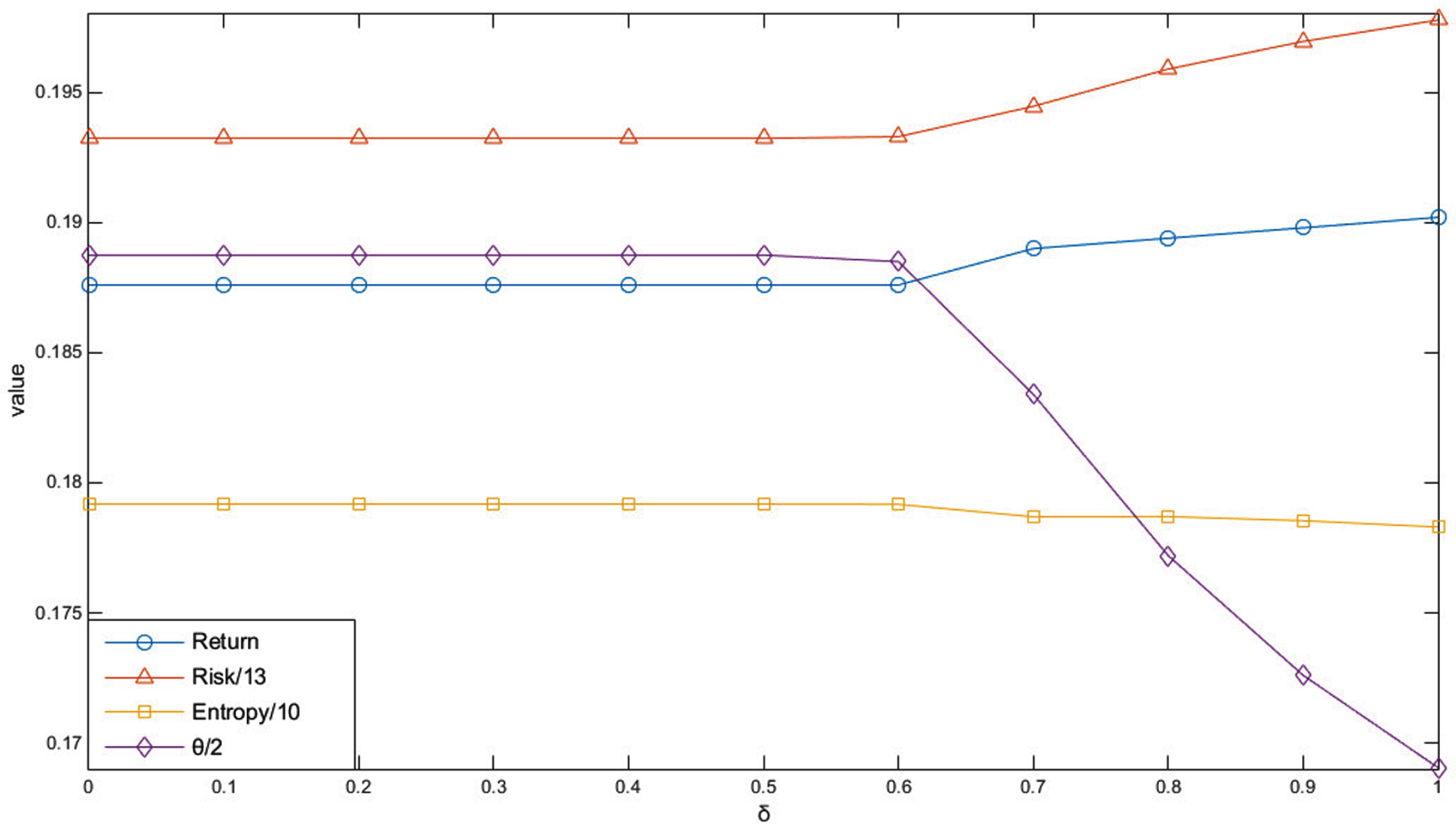
The return, risk (/13), Shannon entropy (/10), θ(/2) of Model (32).
From Tables 10 11 and Figs. 6 7, we can find that: When δ ⩽ 0.5, there is no change in the optimal portfolio strategy. The reason is that PCC = 0 .5890 ⩾ δ when δ ⩽ 0.5. In other words, Model (32) can provide investors with a strategy that satisfies at least 58% of their preference. When δ ⩾ 0.5, the return and risk obtained by Model (32) increase if δ increases. However, the sensitivity of return to δ is less than that of risk, which makes the value of objective θ decrease. It means that if investors hold a lower tolerance level, the portfolio strategy will be worse, which is rational in reality: the actual optimal portfolio strategy always conflicts with investors’ irrational psychology. The Shannon entropy of the strategy provided by Model (32) decreases slowly when δ increases. In fact, from Table 10 and Fig. 6, we can find that all the assets hold the same investment ratio when δ ⩽ 0.5. In this case, it is easy to prove that the Shannon entropy is at its maximum. When δ ⩾ 0.5, the balance is broken and the value of entropy decreases. The investment ratio allocated to A2 is the maximum at all times. In addition, the investment ratio allocated to A2 increases with the increase of δ when δ ⩾ 0.5. Conversely, the investment ratio allocated to A8 is the minimum and it decreases with the increase of δ when δ ⩾ 0.5. The reason is that the relative fuzzy prospect value of A2 is the highest and that of A8 is the lowest. Thus, if the investors’ tolerance level decreases, A2 would be allocated more investment ratios and A8 would be allocated fewer, which also demonstrates that the definition of prospect consistency coefficient is rational.
In order to better illustrate the advantages and limitations of our proposed model, we compared it with some existing studies:
(i) The Comparison with Zhou and Xu [45]:
In [45], Zhou and Xu proposed a novel model under the intuitionistic fuzzy environment. This model took the investors’ preference for risk into account but ignored the investors’ preference for assets. Comparatively, it seems that our model just focuses on the investors’ preference for assets. In fact, as mentioned in Section 7.1, if the investor is risk averse, they can select small values of α, β and λ to reduce the risk; Otherwise, they can choose a small value for λ and large values for α, β. Thus, our model also takes the investors’ preference for risk into account. Another difference between [45] and our model is that Zhou’s model can provide investors with suitable strategy when the historical data is unavailable, and our model needs sufficient historical data to quantify the return rates of assets.
(ii) The Comparison with Kar et al. [46]:
In [46], Kar proposed a bi-objective portfolio selection model based on fuzzy Sharpe ratio and fuzzy VaR ratio. This study adopted new return measure and risk measure, fuzzy Sharpe ratio and fuzzy VaR ratio, to evaluate the portfolio strategy. Comparatively, the possibilistic mean and variance used in our model are conventional. However, Kar’s model did not consider investors’ preference, whether for risk or assets, which may offer investors portfolio strategies that are inconsistent with their preference.
(iii) The Comparison with Sui et al. [47]:
In [47], Sui set up a possibilistic portfolio selection model with liquidity constraint. This model regarded asset liquidity as fuzzy variable, and then introduced the possibilistic liquidity constraint into portfolio selection model to help investors make better use of their capital. Similar to [45], it also took the investors’ preference for risk into account but ignored the investors’ preference for assets. In addition, from Tables 3 5 in [47], it could be found that Sui’s model may not allocate any investment to a selected asset. In contrast, according to Theorem 4, as long as δ > 0 (i.e. investors are not completely rational) in Model (31), our model can ensure that each asset will be allocated a certain amount of investment and the risk will be dispersed better.
Conclusion
For portfolio selection problem, considering that most studies have taken the investors’ preference for risk into account but ignored the investors’ preference for assets, in this paper, the prospect theory and possibility theory are combined to provide investors with a strategy that satisfies their preference for assets. Firstly, a novel reference point is proposed based on the joint possibility distribution of assets, which can provide investors with a comprehensive impression of these assets. Secondly, the prospect returns and risks of each asset are obtained by calculating the possibilistic mean and possibilistic variance of these assets. In addition, we defined the fuzzy prospect value of asset to denote the score of an asset in investors’ subjective cognition. For it can describe the prospect return rate of an asset under unit risk, it is utilized to rank the assets. On this basis, a prospect asset filtering frame is put forward. This framework can help investors solve the problem of how to select a certain number of assets from a large set. Especially, according to the rule of Selection Operation, it can ensure that all the selected assets have the highest scores, i.e. the highest fuzzy prospect values to satisfy investors’ preference.
In order to measure the consistency between a portfolio strategy and investors’ preference with range [0, 1], a new definition called prospect consistency coefficient is proposed. And then, considering that portfolio selection model may provide investors with strategies inconsistent with their preference for assets, we introduce the prospect consistency constraint with a parameter into the model. This parameter is used to describe investors’ tolerance level on the deviation of a portfolio strategy from their preference. Within the investors’ tolerance level, the model will provide investors with an optimal strategy to make profit and reduce risk as much as possible. Furthermore, it is pointed out that with the increase of investors’ tolerance level, the portfolio strategy provided by the model will be better, which indicates that the investors’ preference for assets is one of the irrational psychologies. Finally, a numerical example and the sensitivity analysis are given to show the efficiency of our proposed method. The results point out that compared with the general model, our model can not only better satisfy investors’ preference for assets, but also disperse risk effectively.
In the future, we will combine prospect theory with multi-period investment and then study the problem of multi-period investment based on investors’ preference for assets.
Footnotes
Acknowledgments
This research was supported by the “Humanities and Social Sciences Research and Planning Fund of the Ministry of Education of China, No. x2lxY9180090”, “Natural Science Foundation of Guangdong Province, No. 2019A1515011038”, “Soft Science of Guangdong Province, and No. 2018A070712006, 2019A101002118”, and “Fundamental Research Funds for the Central Universities of China, No. x2lxC2180170”. The authors are highly grateful to the referees and editor in-chief for their very helpful comments.