Deep ganitrus algorithm for speech emotion recognition

Abstract

Human emotion recognition with the evaluation of speech signals is an emerging topic in recent decades. Emotion recognition through speech signals is relatively confusing because of the speaking style, voice quality, cultural background of the speaker, environment, etc. Even though numerous signal processing methods and frameworks exists to detect and characterize the speech signal’s emotions, they do not attain the full speech emotion recognition (SER) accuracy and success rate. This paper proposes a novel algorithm, namely the deep ganitrus algorithm (DGA), to perceive the various categories of emotions from the input speech signal for better accuracy. DGA combines independent component analysis with fisher criterion for feature extraction and deep belief network with wake sleep for emotion classification. This algorithm is inspired by the elaeocarpus ganitrus (rudraksha seed), which has 1 to 21 lines. The single line bead is rarest to find, analogously finding a single emotion from the speech signal is also complex. The proposed DGA is experimentally verified on the Berlin database. Finally, the evaluation results were compared with the existing framework, and the test result accomplishes better recognition accuracy when compared with all other current algorithms.

Keywords

Speech signal emotion recognition deep analysis deep ganitrus algorithm recognition accuracy

1 Introduction

Human speech is different forms of emotions, faces, and gesture speeches for communication that take both the speaker’s communication and emotional conditions [1]. People have an average ability to diagnose the speakers’ emotions from their speech signals, which focuses on consequently finding the emotional state from the distinct category of the human speech signal, which brings the linguistic statistics and likewise their gender, age, origin, and expressive conditions [2]. This structure has made numerous probable effects on the human-computer interface (HCI) [3, 4]. Spontaneous speech emotion recognition (SER) has been utilized in multiple real-life gadgets to examine and identify all emotions in call centers.

SER is mainly implemented to understand the emotional state of the speaker [5]. SER has several applications like robot interaction, e-learning, online games, call centers, etc. For example, in an e-learning classroom, emotion recognition will help identify the students’ emotional state [6]. Whether the topic is understandable or not, it also increases techniques for handling feelings inside the studying surroundings [7]. Numerous advantages make SER superior technology for computing. Likewise, the benefits have several implementation complications, such as a suitable emotional database, feature extraction efficiency, classification algorithms, and so on [8].

Along with this, SER performs three main functionalities for emotion recognition, namely, preprocessing, feature extraction, and emotion classification. In preprocessing, incomplete and other unwanted noise signals are removed for better credit. The feature extraction is then performed; the extracted feature ought to create a more remarkable effect and capacity to speak to various emotions existing in speech signals [9]. In general, the feature extraction procedure is performed at three distinct levels: edge, fragment, and utterance from the speech signal [10]. Typical toolboxes are available to mine speech signal features, similar to PRAAT, APARAT, Open SMILE, and Open EAR [11]. The mined features are marked with different statistics for all emotions; then, multiple classifiers were employed to diagnose the feeling through classification. It usually takes the whole emotion sentence as units for feature extraction, and the extracted features are considered as a piece of characteristics [12, 13]. The emotional speech with no expressive features is then classified based on explicit signal distribution [14]. By following this procedure, unwanted features are also considered for the evaluation, and finally, the accuracy gets diminished.

The above-mentioned previous research focused on a large portion of the speech processing techniques using the hidden Markov model (HMM) and Gaussian mixture model (GMM) etc., to characterize feelings. The serious issue with these strategies is that they require point-by-point presumptions about the information conveyance and model boundaries. Additionally, neural network-based characterization models need preparing information for better arrangement; however, they contain low-level elements, nearby requests, and intrinsic qualities, which are hard to deal with in acoustic models. Generally speaking, the algorithm ought to be planned by (i) selecting the main signal features to include the detailed data to effectively perceive by any other model and (ii) the reasonable determination of samples for training a classification model. In recent research, DNN [15] has a unique achievement in speech and image processing, even though only limited research has been done on SER [16]. In [17] the authors have proposed an SER system based on the gender of the speaker using residual convolutional neural network (R-CNN) and is independent of acoustic features of speech. But the limitation of the algorithm is that it is unable to operate in real time and has large computational power. The deep CNN and discriminant temporal pyramid matching in [18] is used for bridging the gap between the low level features and the subjective emotions. The algorithm has a drawback that it is not capable of dealing with continuous dimension SER. Bidirectional long short term memory with directional self-attention (BLSTM-DSA) in [19] demonstrate that the directional analysis is better at SER.

It is found that DNN has a massive benefit in SER. Human recognition can have inaccurate results; so here we have implemented an automated five-layered network-based framework to train and recognize emotions with high accuracy. This work proposes a classifier framework to perceive emotions. Unfortunately, there are no hypothetical conditions to notice the features that openly speak about a speech signal’s emotions. Consequently, this approach searches about concentration in the manner to restrain to defeat existing difficulties.

There are five sections in this paper. Section 1 and Section 2 gives the introduction and related work, respectively. It discusses the motivation for carrying out this work and describes the complexities involved in SER. The experimental technique, feature extraction technique, and databases employed in the proposed work are all covered in Section 3. It also explains the proposed DGN and DGA methods. Section 4 shows how well the suggested detector performs in terms of specific outcomes. This also includes a comparison of the proposed study to previous work. Section 5 gives the conclusion.

2 Related works

This section reviews the latest work done in SER. Table 1 gives the literature review with various scopes and findings.

Table 1
Literature review

Author name Methodology Database used Scope Findings Future work

and year

Kwon, 2019 [20] An artificial intelligence-assisted deep stride convolutional neural network (CNN) architecture. •Interactive Emotional Dyadic Motion Capture (IEMOCAP) •Ryerson Audio-Visual Database of Emotional Speech and Song (RAVDESS) datasets SER (Anger, Clam, Disgust, Fear, Happy, Neutral, Sad and Surprise) Accuracy: •79.5% on RAVDESS. •81.75% on IEMOCAP.

Vryzas et al., 2020 [21] Convolutional Neural Networks (CNN) architecture. Acted Emotional Speech Dynamic Database (AESDD). continuous SER (Anger, Disgust, Fear, Happiness, and Sadness) Accuracy: •69.2% on AESDD. Transfer learning with different languages.

Sajjad et al., 2020 [22] •Critical sequence segment selection: Redial Based Function Network (RBFN) •Feature extraction: CNN •Learning: Deep Bi-Directional Long Short-Term Memory (BiLSTM) •IEMOCAP •EMO-DB •RAVDESS SER (anger, sad, happy, neutral, surprise, disgust, frustrated, excited, and fearful) Accuracy: •72.25 on IEMOCAP •85.57% on EMO-DB •77.02% on RAVDESS SER using DBN, GRU, and spike networks.

Mohamed et al., 2020 [23] Concealment RNN (ConcealNet) RECOLA dataset Audio Packet Loss Concealment (PLC) and corresponding emotions predictions Arousal: dropped from 76.93% to 75.99 %, Valence: dropped from 43.18% to 39.81 %. Generative approaches such as variants of generative adversarial topologies or variational solutions

Chen et al., 2020 [24] The two-layer fuzzy multiple random forests (TLFMRF) •CASIA corpus •Berlin EmoDB SER (fear, happy, neutral, sad, and surprise) Computation time: 0.0579s Accuracy: •83.14% on CASIA. •85.61 % on EmoDB. Human-robot interaction

Mohamed et al., 2020 [25] Markov Chain model RECOLA corpus Automatic speech emotion recognition Observed the effects of frame loss in SER. Packet Loss Concealment (PLC).

Zheng et al., 2020 [26] Convolutional Recurrent Neural Network (CRNN) IEMOCAP corpus Multi-Level Speech Emotion Recognition Accuracy: 75% on IEMOCAP Personalized network model structure

Siriwardhana et al., 2020 [27] Shallow Fusion of Self Supervised Learning (SSL) •IEMOCAP •CMU-MOSEI •CMU-MOSI Multimodal emotion recognition Accuracy with two classes: •88.04% on CMU-MOSEI •88.275% on CMU-MOSI Natural Language Processing (NLP)

Parthasarathy et al., 2020 [28] Lad+UL+MTL MSP-Podcast corpus. Semi-Supervised Speech Emotion Recognition. Relative gains of 16.1% for arousal, 40% for valence, and 5.5% for dominance over the STL baseline. Ladder network architectures for predicting valence scores.

Shukla et al., 2020 [29] Stochastic Deep Conviction Network (SDCN) EMODB SER (anger, disgust, fear, happiness, sadness and neutral). Accuracy: 95% Recognition rate: 98% Computation time: 23 seconds Diversity in the ensemble of speech recognition.

Author name	Methodology	Database used	Scope	Findings	Future work
Kwon, 2019 [20]	An artificial intelligence-assisted deep stride convolutional neural network (CNN) architecture.	•Interactive Emotional Dyadic Motion Capture (IEMOCAP) •Ryerson Audio-Visual Database of Emotional Speech and Song (RAVDESS) datasets	SER (Anger, Clam, Disgust, Fear, Happy, Neutral, Sad and Surprise)	Accuracy: •79.5% on RAVDESS. •81.75% on IEMOCAP.
Vryzas et al., 2020 [21]	Convolutional Neural Networks (CNN) architecture.	Acted Emotional Speech Dynamic Database (AESDD).	continuous SER (Anger, Disgust, Fear, Happiness, and Sadness)	Accuracy: •69.2% on AESDD.	Transfer learning with different languages.
Sajjad et al., 2020 [22]	•Critical sequence segment selection: Redial Based Function Network (RBFN) •Feature extraction: CNN •Learning: Deep Bi-Directional Long Short-Term Memory (BiLSTM)	•IEMOCAP •EMO-DB •RAVDESS	SER (anger, sad, happy, neutral, surprise, disgust, frustrated, excited, and fearful)	Accuracy: •72.25 on IEMOCAP •85.57% on EMO-DB •77.02% on RAVDESS	SER using DBN, GRU, and spike networks.
Mohamed et al., 2020 [23]	Concealment RNN (ConcealNet)	RECOLA dataset	Audio Packet Loss Concealment (PLC) and corresponding emotions predictions	Arousal: dropped from 76.93% to 75.99 %, Valence: dropped from 43.18% to 39.81 %.	Generative approaches such as variants of generative adversarial topologies or variational solutions
Chen et al., 2020 [24]	The two-layer fuzzy multiple random forests (TLFMRF)	•CASIA corpus •Berlin EmoDB	SER (fear, happy, neutral, sad, and surprise)	Computation time: 0.0579s Accuracy: •83.14% on CASIA. •85.61 % on EmoDB.	Human-robot interaction
Mohamed et al., 2020 [25]	Markov Chain model	RECOLA corpus	Automatic speech emotion recognition	Observed the effects of frame loss in SER.	Packet Loss Concealment (PLC).
Zheng et al., 2020 [26]	Convolutional Recurrent Neural Network (CRNN)	IEMOCAP corpus	Multi-Level Speech Emotion Recognition	Accuracy: 75% on IEMOCAP	Personalized network model structure
Siriwardhana et al., 2020 [27]	Shallow Fusion of Self Supervised Learning (SSL)	•IEMOCAP •CMU-MOSEI •CMU-MOSI	Multimodal emotion recognition	Accuracy with two classes: •88.04% on CMU-MOSEI •88.275% on CMU-MOSI	Natural Language Processing (NLP)
Parthasarathy et al., 2020 [28]	Lad+UL+MTL	MSP-Podcast corpus.	Semi-Supervised Speech Emotion Recognition.	Relative gains of 16.1% for arousal, 40% for valence, and 5.5% for dominance over the STL baseline.	Ladder network architectures for predicting valence scores.
Shukla et al., 2020 [29]	Stochastic Deep Conviction Network (SDCN)	EMODB	SER (anger, disgust, fear, happiness, sadness and neutral).	Accuracy: 95% Recognition rate: 98% Computation time: 23 seconds	Diversity in the ensemble of speech recognition.

3 Proposed methodology

Nowadays, communication with computing hardware has grown increasingly ‘chatty.’ The SER hardware is aware of our emotions and responds to them the same way a human conversational companion would. In the proposed work, an appropriate classification scheme to improve emotion accuracy, which is a mix of four emotions: anger, fear, sadness, and disgust (in other words, stress, anxiety, and depression), is discussed. Recognizing these types of emotions is challenging in terms of precision. As a result, we present a novel deep ganitrus algorithm (DGA) for detecting human emotions and affective states from speech, inspired by Elaeocarpus Ganitrus’ notion [30]. Elaeocarpus Ganitrus bead is a round bead found in the fruits of Elaeocarpus Ganitrus. The number of “mukhi’s” –the clefts and furrows –on the surface of the Rudraksha beads determines their classification. Although the scriptures mention 1 to 38 mukhis, Rudraksha of 1 to 14 mukhis is more commonly used. The most popular Rudraksha bead is the five-faceted or panche Mukhi rudraksha bead. Higher mukhis, or faces, are pretty rare. Each bead has a varied effect depending on the quantity of mukhis it contains.

Stress, anxiety, sadness, palpitation, nerve pain, and psychosomatic disorders are all treated with it in traditional medicine. It lowers the body’s internal temperature and relaxes the mind. The seed kernel (fruit stone) is delicious, cooling, and emollient. The prevalent beads within are rigid and robust, with all the earmarks of being comparative in vision; but, when we deep classify it by the number of lines, they are assorted. The beads, on the other hand, are the most impressive medicinal component.

Similarly, human beings experience different types of emotions. Regardless, SER is unquestionably not an easy task. For example, when we receive a voice signal, it might have a single emotion. However, a closer examination reveals that it may elicit a range of feelings. As shown in Fig. 1, the proposed DGA method employs many procedures to distinguish various emotions. Elaeocarpus Ganitrus appears in various faces simultaneously; similarly, different emotions arise in the voice signal simultaneously, which can be detected by extracting additional features. The proposed DGA employs independent component analysis with the Fisher criterion to assess the voice signal’s unique emotion properties. To categorize distinct emotions based on Elaeocarpus Ganitrus classification, the proposed DGA uses a greedy wise layer learning of DBN with wake-sleep. Deep learning algorithms can perceive complex structures and features without manual feature extraction and deal with unlabeled data. Here some of the most effective, quicker, and optimized results are combined, thereby providing algorithms with the DBN approach to produce more accurate emotion recognition in the shortest possible time and with the lowest possible error rate. Since some emotions are easily detectable, it might be challenging to differentiate single emotion from a cluster of emotions such as anger, joy, sadness, fear, contempt, boredom, and neutrality.

Fig. 1

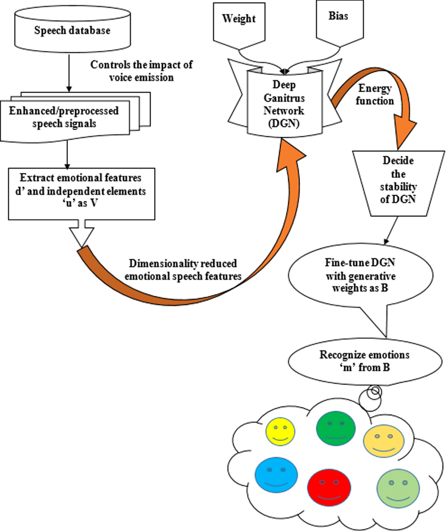
Flow diagram of proposed deep ganitrus algorithm.

Based on greedy layer-wise learning, the proposed system is aimed to perceive the emotions stated above accurately. The sections below provide a quick overview of how to achieve high accuracy while identifying various emotions.

3.1 Proposed deep ganitrus network (DGN)

In Fig. 1, DGA mainly comprises DGN as a classifier and independent component analysis with fisher criterion for feature extraction. DGN incorporates various random subspaces with a deep belief network. The wake-sleep algorithm is used for emotion classification to improve the naturalness and efficiency of spoken human-machine interfaces by exploiting extracted attributes.

3.2 Feature extraction: independent component analysis (ICA)

ICA is a type of blind source separation (BSS) method for decomposing data into underlying informative constituents, including images, sounds, telecommunication channels, or stock market prices [31]. The word “blind” refers to the ability of such approaches to divide data into source signals despite knowing little about the nature of those source signals. Independent component analysis divides a set of signal mixes into statistically independent component signals or source signals, as the name suggests. ICA is based on the essential, generic, and the realistically reasonable premise that various signals from different physical processes (for example, other persons speaking) are statistically independent. ICA exploits the fact that the consequence of this assumption can be inverted, resulting in a new assumption that is logically unjustified yet works in practice. If statistically independent signals can be recovered from signal mixes, they must be from different physical processes (e.g., other people speaking). As a result, ICA splits signal mixtures into statistically independent signals.

Principal component analysis (PCA) and factor analysis (FA) are two standard methods for evaluating substantial data sets. PCA and FA find signals with a considerably weaker property than independence, but ICA identifies a group of independent source signals. PCA and FA, in particular, look for a group of uncorrelated signals.

In ICA, there are two fundamental assumptions. First, we need statistically independent and non-Gaussian hidden separate components to find them. In linguistics, independence means that knowledge about x does not provide you with knowledge about y, and vice versa. Second, ICA can offer the ability to extract emotional features as independent variables. Third, unlike PCA, which focuses on maximizing the data point’s variance, the ICA focuses on independence. Third, ICA is a method for isolating additive subcomponents from a multivariate input. This is accomplished by assuming that the discrete components are non-Gaussian signals with statistical independence. Here n is linear mixtures, x = x₁, …… … . . , x_n is a random vector of n independent components, and s is a random vector with elements s₁, s₂, . . . . . . , s_n $x_{j} = a_{j 1} s_{1} + a_{j 2} s_{2} + \dots \dots \dots + a_{jn} s_{n}, for all j$ (1) $x = A s : Columns of matrix A denoted by a_{j}$ (2) $x = \sum_{i = 1}^{n} a_{i} s_{i}$ (3) Equation 2 is called the ICA model. ICA model is a generative model having independent latent variables. The independent component is obtained by: $S = Wx$ (4) where, W is the inverse of matrix A

3.2.1 ICA with fisher criterion

The proposed deep ganitrus ICA with fisher criterion [32] reveals the hidden factors that underlie sets of random variables and measurements and provide a reduced dataset with valuable features. Fisher criterion is the supervised criteria. It is being used to eliminate features that are noisy or unnecessary. However, it does not take into account feature redundancy. For example, if two feature vectors are identical and have high Fisher values, they will be selected with high redundancy. The ICA method investigates the relationship between features and eliminates duplicated features [33], but it cannot discern between noisy and valuable features.

3.2.2 Pre-selection using fisher criterion

The categorization of Z classes is taken. Let m_j be the training samples (vectors) { $p_{1}^{j}$ , $p_{2}^{j}, \dots \dots \dots, p_{m_{j}}^{j}$ } for class j, (j = 1, 2 . . . Z). The apriori probability of class Z is given as: $P_{j} = \frac{m_{j}}{\sum_{j = 1}^{Z} m_{j}}$ (5) The mean of the class is calculated as $\hat{μ_{j}} = \frac{1}{m_{j}} \sum_{n = 1}^{m_{j}} P_{n}^{j}$ (6) And the gross mean is given as $\hat{μ} = \sum_{j = 1}^{Z} P_{j} \hat{μ_{j}}$ (7) The covariance matrix of the class Z is evaluated as $\hat{C_{j}} = \frac{1}{m_{j}} \sum_{n = 1}^{m_{j}} (P_{n}^{j} - \hat{μ_{j}}) {(P_{n}^{j} - \hat{μ_{j}})}^{T}$ (8) The covariance matrix of within class C_ω and between classes C_b is calculated as $C_{ω} = \sum_{j = 1}^{Z} P_{j} \hat{C_{j}}$ (9) $C_{b} = \sum_{j = 1}^{Z} P_{j} (\hat{μ_{j}} - \hat{μ}) {(\hat{μ_{j}} - \hat{μ})}^{T}$ (10) The separability of a class of a feature set is evaluated as $G_{K} = trace ({C_{ω}}^{- 1} C_{b})$ (11) The ‘Fisher rate’ λ_F $λ_{F} = \frac{{C_{b}}^{(F)}}{{C_{ω}}^{(F)}}$ (12)C_b^(F) and C_ω^(F) are the Fth element of C_b and C_ω respectively and it can be evaluated from the data from a single feature. C_b and C_ω provides the essential emotion features with applied feature extraction and dimensionality reduction.

Regarding feature pre-selection, simply calculate each feature’s Fisher criterion, sort the features in decreasing order of criterion values, and choose the features with the highest Fisher values. In contrast, the features with the lowest Fisher values are discarded. Even though the single-feature Fisher criterion ignores the joint separability of multiple features, it can maintain all discriminant features by deleting only irrelevant/noisy features. The Fisher criterion is almost zero.

3.3 Proposed deep ganitrus algorithm

The following are the steps of the proposed algorithm:

Initialize Fisher Criterion in ICA (ICA-FC)): For each feature in the first set, calculate the Fisher criteria value. Sort the features by Fisher rate in decreasing order using Equations (5)–(7). Identify the leading characteristics until the cumulative Fisher value percentage surpasses 99%. The u /bold> UD comprising emotional feature ‘u’ and independent elements as ‘d’ (ICA) using Equations (1)–(4)

Initialize DBN-WS: A DBN is trained in two stages: the greedy layer-wise pre-training and fine-tuning. The input data is used to train the first-layer RBM in the pre-training step, V (i = 1 to n). The concealed unit values are then utilized as training data for the RBM in the following layer.

For training, features are extracted from V, and random subspaces are generated Ri (i = 1 to n)

Create DBN from Ri

Use V to train the layers of RBM using a contrastive divergence algorithm. Obtain pre-learned parameters w_ij, b.

3.4 Restricted Boltzmann machines

Deep Belief Networks (DBN) are generative probabilistic models with several layers of hidden variables, each layer capturing significant high-order correlations between hidden characteristics in the layer below. These models have been effectively implemented in various application domains due to efficient greedy methods for learning and approximate inference. The fundamental building component of a DBN is RBM which is a bipartite undirected graphical model. It shares attributes with individual levels of a DBN. The next concern is usually how to train the model once it has been developed. Since this is a probability model, we frequently utilize the maximum-likelihood method for training the model’s parameters. Regrettably, the probability of data underneath the model is only known up to the partition function, a computationally tricky normalizing constant. Model selection and model complexity control would both benefit from a reasonable estimate of the partition function. Hinton suggested that the contrastive divergence (CD) [34, 35] method circumvent this difficulty by approximating a distinct function’s gradient.

A Boltzmann machine [36] is a network of stochastic binary units that are symmetrically connected. It has a set of visible units S, m ∈ { 0, 1 } ^S as well as a set of hidden units T, h ∈ { 0, 1 } ^T. The state, h’s energy is defined as: $E (m, h; δ) = - c^{'} h - d^{'} m - m^{T} Pm - h^{T} Qh - m^{T} Rh$ (13)

Where δ ={ R, P, Q, c, d } are the model parameters, and visible-to-visible, visible-to-hidden, and hidden-to-hidden symmetric interaction terms are represented by P, R, and Q, respectively. The well-known Restricted Boltzmann machine model is recovered by setting P = 0 and Q = 0. The energy is given as $E [m, h; δ] = c^{'} h - d^{'} ϑ - m^{T} Rh$ (14) $δ = {R, c, d}$ (15)

RBM generates a bipartite graph since they only have connectivity between a hidden and visible unit. The Gibbs distribution is the most straightforward and most popular approach for converting a set of random energies into a collection ranging from 0 to 1 whose sum is 1. Therefore the probability which the model allocates to a visible vector m is: $\begin{matrix} P (m; δ) & = \sum_{h} \frac{exp (- E (m, h; δ))}{D (δ)} \\ = \frac{\sum_{h} exp ((- E (m, h; δ))}{\sum_{m} \sum_{h} exp (- E (m, h; δ))} \end{matrix}$ (16) The Maximum-likelihood (ML) learning of the parameters ø given, i.i.d. samples $M = {m^{(j)}}_{j = 1}^{Y}$ be done by gradient descent: $ø^{(μ + 1)} = ø^{(μ)} + {γ \frac{\partial L_{L} (ø; ϑ)}{\partial ø} |}_{(μ)}$ (17) μ is the learning rate which can vary, and the average log-likelihood is: $L_{L} (ø; V) = \frac{1}{Y} \sum_{j = 1}^{Y} log p (m^{(j)}; ø)$ (18) The log-likelihood gradient could be expressed in the form: $\begin{matrix} \frac{\partial log p (m; ø)}{\partial ø} = - \sum_{h} p (h | m) \frac{\partial E (m, h; ø)}{\partial ø} \\ + \sum_{ϑ, h} p (m, h) \frac{\partial E (m, h; ø)}{\partial ø} \end{matrix}$ (19)

Table 2

Description of variables for CD algorithm

S. No	Parameters	Description
1	m ₁	A representative sample from the RBM’s data distribution
2	τ	SGD learning rate in CD
3	R	The weight matrix of the RBM
4	c	Hidden units, RBM offset vector
5	d	Input units, RBM offset vector
6	σ	Sigmoid function in the neural network

The Markov chain Monte Carlo (MCMC) method has the advantage of being adaptable to a wide range of distribution types p (m ; ø). However, because executing the Markov chain to equilibrium might take a significant number of steps, and there is no guaranteed way for determining whether stability has been attained, it is often relatively slow. The substantial variance in the predicted gradient is another problem.

In [37], Hinton suggested the contrastive divergence (CD) approach, which emulates the gradient of a different function to circumvent the complexity of estimating the log-likelihood gradient. The Kullback-Leibler divergence is minimized via machine learning. $KL (p_{0} | | p_{\infty}) = \sum_{ϑ} p_{0} (m) log \frac{p_{0} (m)}{p (m, h; ø)} .$ (20) wherthe data distribution is p₀ (ϑ) and the model distribution is p_∞ (ϑ, h ; ø). The gradient of the differences between two divergences is roughly follow by contrastive divergence (CD) learning: $C D_{k} = KL (p_{0} | | p_{\infty}) - KL (p_{k} | | p_{\infty})$ (21)

The Markov chain is started at the data distribution p₀ and operated for a limited number of steps (e.g., n = 1) in CD learning. This considerably decreases the calculation per gradient step and the variance of the computed gradient, and investigations indicate that it yields accurate parameter assessments.

The CD algorithm for training RBM is described below:

For all hidden units, y do

Calculate p (h_1,y = 1|m₁) = σ (∑_xR_xym_1,x + c_y)

Sample h_1,y∈ { 0, 1 } from p (h_1,y = 1|m₁)

End For

For all visible units, x do

Evaluate p (m_2,x = 1|h₁) = σ (∑_yR_xyh_1,y + d_x)

Sample m_2,y∈ { 0, 1 } from p (m_2,x = 1|h₁)

End For

For all hidden units, y do

Compute p (h_2,y = 1|m₂) = σ (∑_xR_xym_2,x + c_y)

End For

$R = R + τ (h_{1} ϑ_{1}^{'} - p (h_{2} = 1 | m_{2}) m_{2}^{'}$ d = d + τ (m₁ - m₂) c = c + τ (h₁ - p (h₂ = 1|m₂)

3.5 Deep belief network wake-sleep algorithm for classification

DBNs are generative models with several layers of hidden units that are probabilistic. RBMs are frequently used to build DBNs, which are built by stacking and training them in a greedy layer-by-layer fashion that is repeated several times. Figure 2 depicts a five-layer DBN. From the HL in the layer below, each layer of the DBN may takes high-order features. The top two layers will continue to create the RBM, whereas the bottom levels will form the directional sigmoid belief network.

Fig. 2

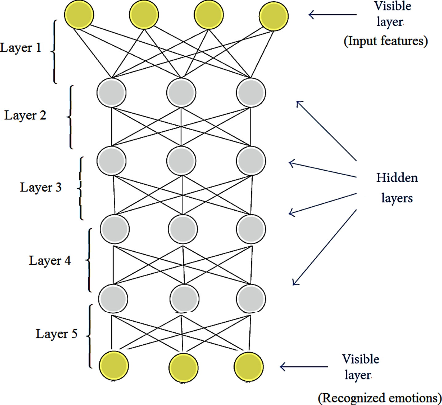
Five-layer pre-trained network architecture.

To train a DBN, a greedy layer-wise pre-training and fine-tuning approach is utilized. The first layer of RBM is trained utilizing input data in the pre-training stage, after which the outputs of its hidden units are employed as training data for the RBM in the following layer, and so on. As seen in Algorithm 1, the process can be applied layer by layer until a deep model is created. By requiring just, a single bottom-up pass to deduce the values of the top-level hidden variables, this learning approach ensures efficient approximated inference. The DBN can indeed be fine-tuned by employing supervised learning algorithms, including BP and SGD, after greedy learning in the first stage, and then it will be suitable for classification and recognition.

For training, the derivative of the emotion recognition is determined by considering the model boundaries ‘R’ and ‘b’. By approximating the gradient of the objective function R, the RBM update of the weight and bias are as follows: $Δ R = \in (E X_{e_{data}} [m q^{P}] - E X_{e_{recog}} [m q^{P}])$ (22) $Δ b^{1} = \in (E X_{e_{data}} [q] - E X_{e_{recog}} [q])$ (23) $Δ b^{2} = \in (E X_{e_{data}} [m] - E X_{e_{recog}} [m])$ (24)

EX_{e
_data} [ .]- The expectation of the joint distribution of accurate data.

EX_{e
_recog} [ .]- The expectation concerning the reconstructions.

∈-Learning rate

The joint distribution function of DBN with L layers, m visible vectors, and lth hidden variable h^l (l = 1, 2 . . . L) $\begin{matrix} P (m, h^{1}, h^{2}, \dots \dots, h^{l}) = (\prod_{l = 1}^{L - 1} P (h^{l - 1} | h^{l})) \\ P (h^{L - 1} | h^{L}) \end{matrix}$ (25) Where, m = h⁰, $(\prod_{l = 1}^{L - 1} P (h^{l - 1} | h^{l}))$ gives the directed sigmoid belief network and P (h^L-1|h^L) is the joint distribution and is defined by the RBM in the top two layers. $P (h^{l - 1} | h^{l}) = σ (c^{l} + h^{l} R^{l^{T}}),$ (26) $P (h^{l} | h^{l - 1}) = σ (d^{l} + h^{l - 1} R^{l}),$ (27) $P (h^{L - 1} | h^{L}) = \frac{1}{\sum_{h^{L - 1}, h^{L}} e^{- E (h^{L - 1}, h^{L})}} e^{- E (h^{L - 1}, h^{L})}$ (28) The energy function for the top RBM $E (h^{L - 1} | h^{L}) = - h^{L - 1} R^{L} h^{L^{T}} - h^{L - 1} c^{L^{T}} - h^{L} c^{L^{T}},$ (29)

The posterior Q is calculated since P (h^L-1|h^L) is difficult to calculate and obtain samples from it. Q is used for inference and training so Q (h^l-1|h^l) gives the distribution of lth RBM during training. Except for Q (h^L|h^L-1) which is equal P (h^L|h^L-1) to in topmost RBM, rest all posteriors are approximations.

The wake-sleep algorithm [37] is another unsupervised and quick fine-tuning algorithm for learning a deep discriminative model. When there is no external training signal to match, the concealed units must be forced to extract the underlying structure through some other means. The wake-sleep method aims to learn simple representations to represent but permits the input to be appropriately reconstituted. There are two distinct sets of connections in the neural network. First, the input vector is transformed into characterization in one or more layers of hidden units via bottom-up “recognition” connections. The “generative” connections are then utilized to provide an estimate of the input vector based on its fundamental description using the top-down “generative” connections. The training process for these two sets of connections can be applied to a variety of stochastic neuron types, but stochastic binary units with states of 1 or 0 are considered.

Figure 2 shows the five-layered pre-trained network architecture. Here the input features are the visible layer and the intermediate layers called hidden layers. Finally, the recognized emotions with corresponding weights were obtained as a pre-trained output (visible layer). These pre-trained weights were fine-tuned by applying the wake and sleep phase’s generative and recognition processes, respectively. The pre-trained weights from each enhanced voice signal are given as the input to the deep ganitrus network for the training reason. The feature vector for the training clarification behind existing is of the weight w. The greedy layer-wise way did speech emotion recognition. As appears in Fig. 2, it starts with preparing the primary layer on the input element. The yield of the primary layer is utilized as the contribution of the subsequent layer.

Additionally, the third layer is prepared on the yield of the second layer. Layers 1 to 4 were trained based on each other’s upper layers, and finally, the recognized emotions were gathered based on the previously obtained outcomes. Finally, a deep hierarchical model is built along these lines that take learned weights from low-level weights to get the advanced accurate weight rankings.

In the wake phase (generative), pre-trained weights of layers 1 and 2 were evaluated with regression to eliminate the error/false emotion recognition. B¹, B², B³, B⁴, B⁵, B⁶ produces the recognized weights. In the wake phase, we fine-tune the “generative” weights by $Δ B^{1} = ɛ m_{1}^{1^{T}} (w_{2}^{1} - w_{21}^{1})$ (30) $Δ B^{2} = ɛ m_{2}^{1^{T}} (m_{2}^{2} - m_{21}^{2})$ (31)

In the sleep phase (recognition), pre-trained weights of layers 3 and 4 were evaluated with regression to categorize different types of emotions, and in the sleep phase, the “recognition” was done by $Δ B^{3} = ɛ m_{3}^{3^{T}} (w_{4}^{3} - w_{43}^{3})$ (32) $Δ B^{4} = ɛ m_{4}^{3^{T}} (w_{4}^{4} - m_{43}^{4})$ (33)

Finally, the fifth layer outputs the recognized emotions such as anger, joy, sadness, fear, disgust, boredom, and neutral, obtained by regretting the combination of emotions. i.e., if the speech contains a fusion of emotions, then the emotion recognition attained from the fifth layer be recognized as follows, $\begin{matrix} Δ B^{5} = ɛ (w_{1}^{2^{T}} w_{1}^{3} w_{1}^{4} w_{1}^{5} - w_{2}^{2^{T}} w_{2}^{3} w_{2}^{4} w_{2}^{5} \\ - w_{3}^{2^{T}} w_{3}^{3} w_{3}^{4} w_{3}^{5} - w_{4}^{2^{T}} w_{4}^{3} w_{4}^{4} w_{4}^{5}) \end{matrix}$ (34)

The m and w in the above conditions are sampled according to Equation (25), respectively. The emotions were categorized based on the weight ranking of each emotion. The amount of hidden units in the DGA’s first layer is crucial in lowering the recognition error rate. As it rises, the error rate falls considerably faster than in circumstances when the number of concealed units in subsequent layers rises.

Algorithm 1: Pre-training of deep ganitrus network

Input: Extracted emotion feature sets C_ω and C_b, as initialized parameters, learning rate τ Output: Pre-trained DG network with L layers.

1. for l = 1 to L do

2. Approximate the gradient of the objective function, the RBM update of the weights and biases utilizing ΔR = ∈ (EX_{e
_data} [mq^P] - EX_{e
_recog} [mq^P]), Δb² = ∈ (EX_{e
_data} [m] - EX_{e
_recog} [m])

3. Obtain the joint distribution and energy function using Equations (25)–(27).

4. Get the pre-learned parameters R,c, and d;

5. R(h^l - 1, q¹) is concerned with the transmission of the lth RBM during a learning stage.

6. Estimate the posteriors Q with the exclusion of Q (h^L|h^L-1) corresponding to the true P (h^l| h^l-1).

7. End for

4 Result and discussion

The proposed deep ganitrus algorithm for extracting the distinctive emotion is shown in this section. The person speaking capabilities and the speaker-built-up abilities are recovered separately using our proposed extracting emotional speech elements. When it perceives the last characteristic of the consultant speech emotional feature at length, it analyzes the extracted impassioned data to eliminate the redundant data. Specifically, the proposed emotion detection general implementation is compared with several system-based techniques, and the findings are investigated.

4.1 Experimental setup

This experiment was conducted in a python platform with a system configuration of windows 10 OS, i5 processor with 8 GB RAM. We will use a Python library called Theano, [38] which will provide a significant increase in training performance.

4.2 Dataset description

Suitable dataset selection is essential for any work. In this SER framework, we utilized the Berlin emotional database [39] given in Table 3. It consists of 500 utterances with seven feelings: joy, sadness, disgust, anger, anxiety/fear, neutral, and boredom.

Table 3
EmoDB details

S. No. No. of speakers Gender Age

1 03 M 31

2 08 F 34

3 09 F 21

4 10 M 32

5 11 M 26

6 12 M 30

7 13 F 32

8 14 F 35

9 15 M 25

10 16 F 31

S. No.	No. of speakers	Gender	Age
1	03	M	31
2	08	F	34
3	09	F	21
4	10	M	32
5	11	M	26
6	12	M	30
7	13	F	32
8	14	F	35
9	15	M	25
10	16	F	31

The speech dataset (V_d) is primarily used to extract relevant data from the dataset, which includes changing emotions. Consider the (V_d) data consists of acoustic data with English sounds in various emotions: anger, happiness, sadness, fear, disgust, boredom, neutral, and so on. Each utterance is designated with the V_d and can be spoken in any order. $V_{d} = v_{1} + v_{2} + v_{3} + \dots + v_{n}$ (35)

Every word is spoken by different actors with different emotions, resulting in a list of other datasets. For example, a large pool of 2327 features from EmoDB is extracted, which comprises many features. Specific loudness sensation coefficients (SLSC), MPEG-7 descriptors, total loudness, and Teager energy operator on autocorrelation are among the 602 unique features proposed in this study for establishing emotion recognition.

4.3 Enhancement of input speech signal

During the recording step, loud, inconsistent, and irrelevant information can damage input speech data used for emotion recognition. The emotion classification of this raw data will result in a wrong category and reduced detection accuracy. The input speech signal is upgraded by deleting irrelevant, blank, and corrupted data automatically. Finally, the extraction step is highlighted by a clean signal free of any corruption or recording variance. $m_{e} = m_{1} + m_{2} + m_{3} + \dots + m_{n}$ (36)

Equation (36) denotes the number of features enhanced/automatically preprocessed voice signals as ‘n.’

4.4 Feature extraction

The speech signal is made out of many characteristics that reoccur in remarkable, exuberant singularities [36]. One of the elements that should be used is a feature that is centered around emotional assurance. Elaeocarpus Ganitrus, for example, appears in multiple faces in a single tree, which can be identified by counting the number of lines. Similarly, a single speech signal can include numerous emotions. We must extract the fundamental aspects such as pitch intensity, speaking rate, voice quality, tonal force proportion, and unearthly flux, among others, to define the suitable emotion. Various challenges are always associated with the information dimensions when using factual procedures for extracting pattern recognition’s emotional elements. For example, applying a strategy that works in low-dimensional space to a high-dimensional space is difficult. Furthermore, the technique for dealing with a low-dimensional problem is often low in computing complexity, efficient, and beneficial [40]. In correlation analysis, the extricated datasets are represented by many high-dimensional emotional features, which probably takes considerable time and space.

The extraction of features is done in three stages here. First, the features from the voice signal are recovered as independent components in the first stage. The extended feature vectors, formed of independent static and dynamic features, are collected in the second stage. Finally, if there is one, the final step transforms these upgraded feature vectors into small-scale and robust vectors for the recognizer to use.

It is observed that speech signal mixtures, m_e which is the enhanced input signal consists of ‘n’ number of emotional features signal as described below. $m_{i} = d_{i 1} u_{1} + d_{i 2} u_{2} + \dots + d_{in} u_{n}, for all i^{'}$ (37)

The data variables in the speech signals are thought to be linear mixtures of unknown emotional components. The independent components of the examined data are considered to be non-Gaussian and are mutually independent latent variables. An autonomous speaker scenario is used, and seven emotional classes are considered such as anger, joy, sadness, fear, disgust, boredom, and neutral. Assume that every combination m_i, as well as each independent constituent u_n, is a stochastic variable, rather than a perfect speech signal, in Equation 38. Without losing generality, it may be predicted that each of the aggregate factors and independent components has zero mean.

Using vector-matrix description instead of aggregates, like in the above equation, is significantly more sensible. The emotional components d_ij is denoted by matrix D, and U is the matrix of independent components. $m = DU$ (38) Occasionally the columns of matrix D given as d_j; the equation can also be written as $m = \sum_{i = 1}^{p} d_{i} u_{i}$ (39)

Equation 39 explains how the obtained information is created by collaborating the modules u_i. The unbiased components are inactive, which means they can’t be identified easily. The mixing matrix is also supposed to be unidentifiable. The random vector m is used to estimate both d and v. This vector must be used as close to commonly held assumptions as possible. The starting point is the u_i. component’s statistically unbiased hypothesis.

In this case, non-Gaussian dispersion is employed to calculate the D matrix. The opposite framework is accomplished, state W, after the estimate method of a matrix, and we will obtain the autonomous component vector by $V = UD$ (40)

Where ‘ U’ will be the extricated independent component, the yield of the feature vector will then be used in the event determination optimization, which is done in this work using the Fisher Criterion to reduce emotional speech features.

4.5 Training for speech emotion recognition

In this paper, Theano is used to create the DG network. Theano is a Python package for performing fast numerical computations on either the CPU or the GPU. It’s a major Python deep learning core package that can be used to develop deep learning models directly or wrapper libraries that make the process much easier. It enables us to assess mathematical operations, including multi-dimensional arrays, efficiently. The DG network was initially pre-trained using the greedy layer-wise strategy for deep learning with the wake-sleep algorithm to identify diverse emotions. The Berlin dataset is divided into two parts, using 70 percent of the voice information for training and 30 percent for testing. Almost 100 different hyperparameter combinations have been tried, and the model with the lowest error rate is chosen. Table 4 shows the hyperparameters for generative pre-processing and processing. With a 0.01 learning rate, the layers ran for 475 epochs.

Table 4
Hyperparameters and training statistics of the DGN

Number of layers 5

Units per layer 50

Learning rate 0.01

Number of epochs 475

Recognition accuracy 0.985

Number of layers	5
Units per layer	50
Learning rate	0.01
Number of epochs	475
Recognition accuracy	0.985

4.6 Simulation results

Figure 3 shows an example of a voice signal that can be used to differentiate between various expressions. The goal of automatic emotion detection system research is to develop an effective, real-time framework for mobile phone users, call center workers and customers, automobile drivers, pilots, and other human-machine interaction, subscribers. It has been determined that giving robots emotions is crucial to making them appear and behave more human-like.

Fig. 3

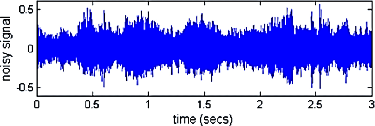
Noisy input voice signal.

Speech signals are crucial in conveying the speaker’s feelings. The speech signal’s emotions change depending on the speaker’s speaking style. As a result, it’s difficult to discern the emotions expressed in the voice signal. By sensing the feelings represented in speech, SER determines the speaker’s emotional states. Figure 4 depicts the preprocessed/enhanced speech signal before the feature extraction stage, where the suggested DGA removes the unwanted noise components naturally.

Fig. 4

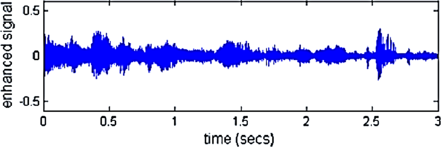
Preprocessed/ Enhanced speech signal.

From this point onwards, the extracted features from the upgraded speech signal, using our recommended feature extraction technique to extract essential features. The deep ganitrus method is used to extract the speech’s significant components. Pre-training and fine-tuning features are provided for determining the appropriate emotion for detecting various feelings and enhancing precision. The clean signal obtained from the improved input speech signal is shown in Fig. 5.

Fig. 5

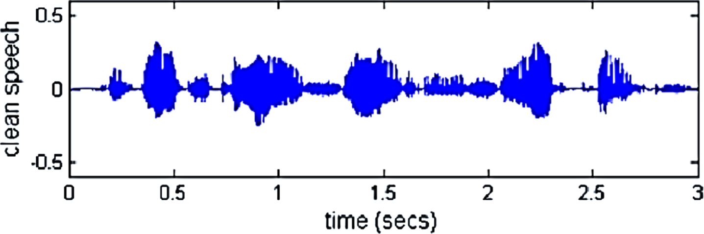
Clean speech signal.

Interpreting the speaker’s emotions through speech signals is more effective because speech provides more meaningful information. Thus, by combining the spatial transformation methods, these significant difficulties in the emotion recognition system can be addressed. For example, people’s speech is full of many emotions, classified as anger, joy, sadness, fear, disgust, boredom, and neutrality. Figure 6 depicts the recognized feelings derived from a single speech input with various ratios. For “Currently at the weekends I always went home and saw Agnes,” the emotions depicted in Fig. 6 were detected.

Fig. 6

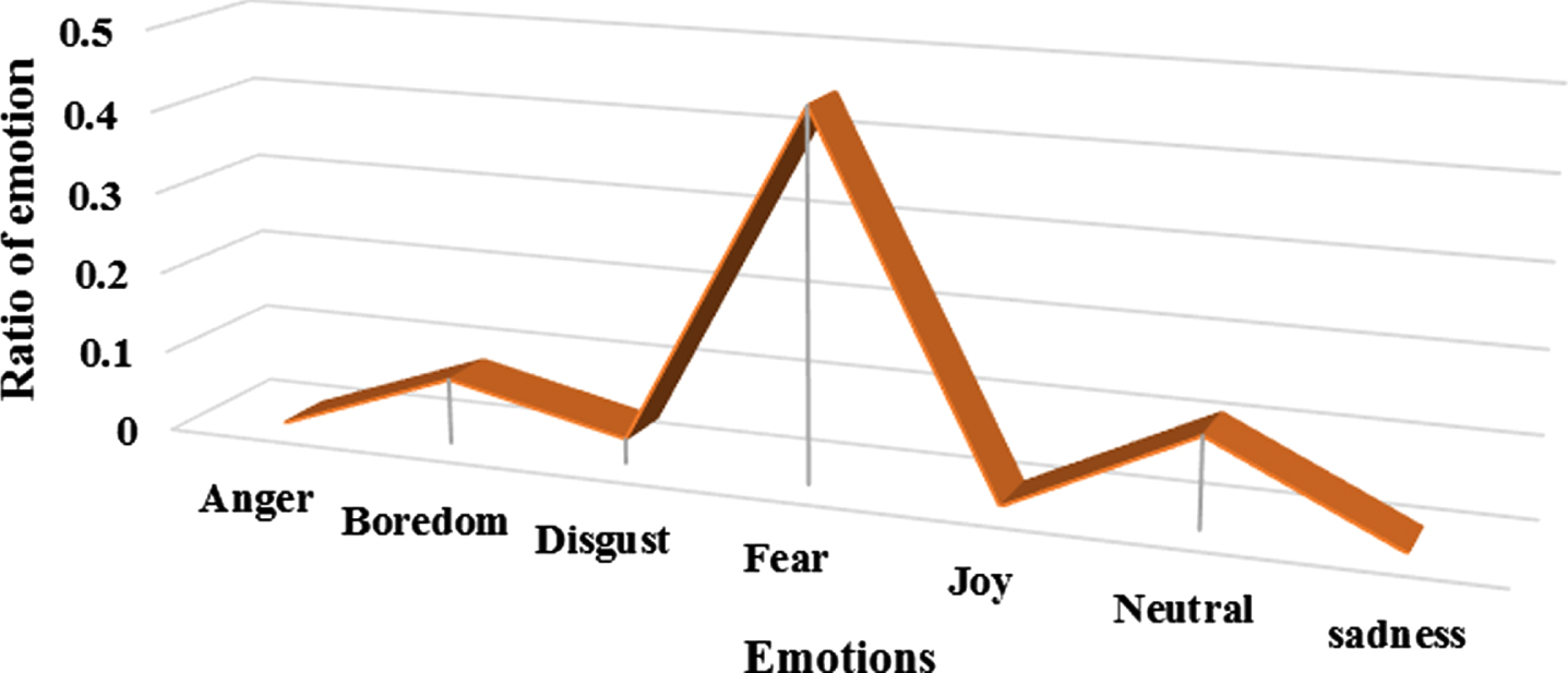
Emotions recognized from a single speech signal.

With the assistance of the Berlin emotional dataset, the proposed DGA architecture is put to the test. The speech emotions in the Berlin database were recorded in various contexts and speech variants, which may include multiple undesired noise signals. Our proposed technique automatically removes unwanted signals. The feature extraction procedure was then applied to the preprocessed/enhanced speech stream. Following that, the recovered features are subjected to emotion recognition using the suggested Deep Ganitrus Algorithm. Finally, it detects the seven emotions contained in the Berlin database.

4.7 Performance analysis

The proposed Deep Ganitrus algorithm is the recognition algorithm, and this way, it is imperative to consider the presentation of the model in idea with the estimations. For instance, false acceptance rate (FAR), false rejection rate (FRR), and precision. The explanation for each assessment metric used in the SER is informed as follows,

i) FAR

It measures the proportion of the falsely perceived feelings to the all-out attempts utilized by the model to sense the emotions, and it has conversed as follows, $FAR = \frac{Number of false recognitions}{Total number of attempts} .$ (41)

ii) FRR

It expresses the proportion of falsely rejected (FR) emotions to the overall attempts utilized by the technique, and it is articulated as follows, $FRR = \frac{Number of false rejections}{Total number of attempts} .$ (42)

i) Accuracy

The accuracy indicates the deviation in enacting the framework with characteristic data, and it is measured in terms of the framework’s positivity and negativity. $Accuracy = \frac{TP + TN}{TP + TN + FP + FN}$ (43)

Table 5 shows the recognition performance analysis of our proposed DGA framework. It offers the performance analysis of different emotions (sadness, joy, neutral, boredom, fear, and disgust) over varying recall/sensitivity, precision, F1-score, FAR, FRR, specificity, and accuracy. Performance measures were calculated for each of the recognized emotions to experiment with the emotion recognition ability of DGA. Proposed DGA recognizes these seven emotions with high accuracy percentages, and the average values are recall: 0.981, precision: 0.982, F1-score: 0.982, FAR: 0.01, FRR: 0.01, specificity: 0.984, and accuracy is 0.985, which is represented graphically in Fig. 7.

Table 5

Recognition performance of DGA over Berlin database

Emotions	Recall/sensitivity	Precision	F1-Score	Specificity	Accuracy	FAR	FRR
Anger	0.975	0.992	0.987	0.989	0.989	0	0
Sadness	0.977	0.963	0.981	0.971	0.982	0.02	0.01
Joy	0.974	0.988	0.971	0.984	0.988	0	0
Neutral	0.981	0.975	0.972	0.988	0.984	0.01	0.02
Boredom	0.992	0.986	0.987	0.983	0.982	0.03	0.01
Fear	0.978	0.993	0.998	0.988	0.989	0	0
Disgust	0.991	0.982	0.979	0.991	0.981	0.03	0.03
Average	0.981	0.982	0.982	0.984	0.985	0.01	0.01

Fig. 7

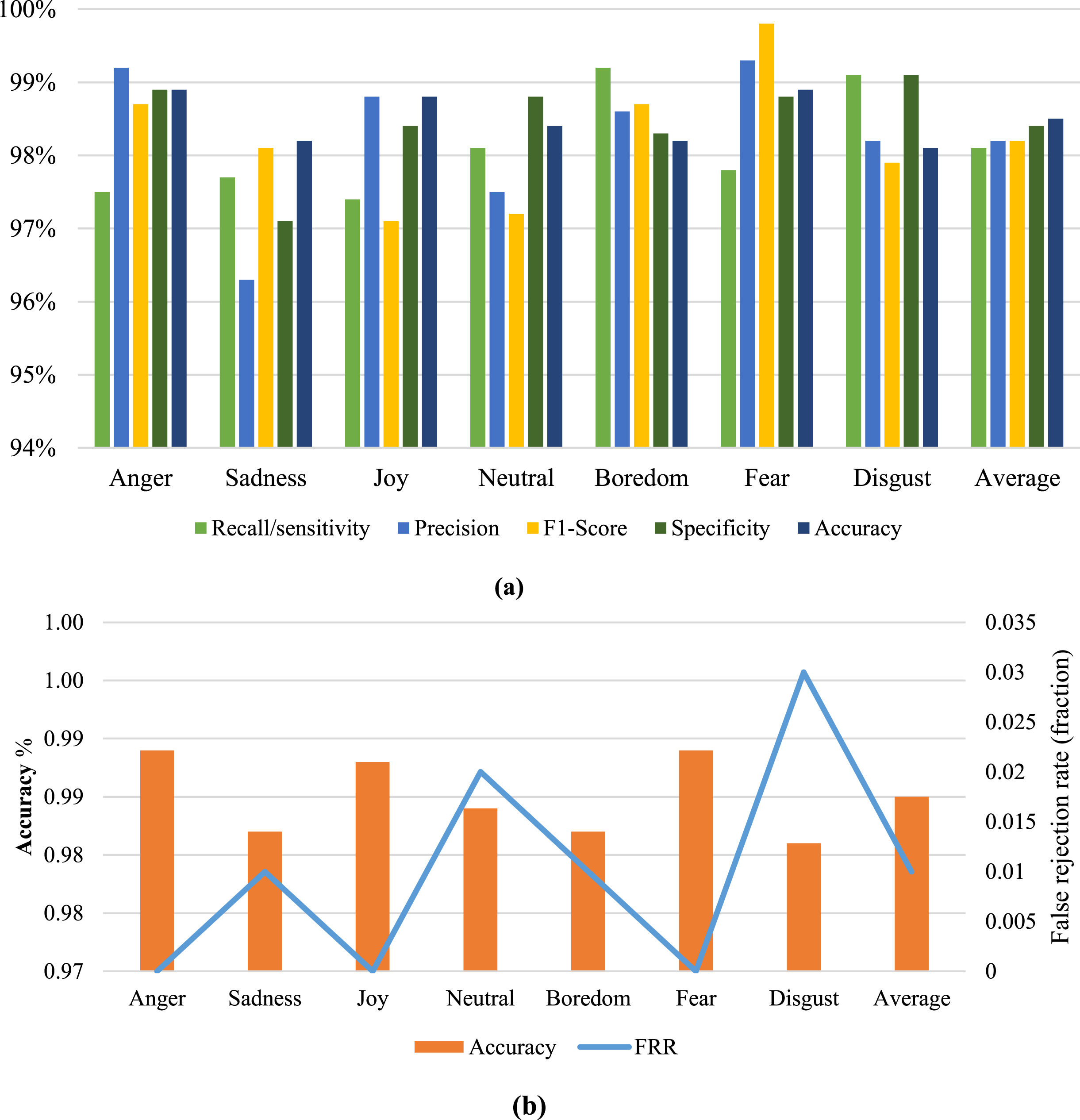
Emotion recognition performance of DGA.

Table 6 shows the confusion matrix for the accuracy % of the Deep Ganitrus Algorithm. The bold values indicated in the matrix represent the highest recognition accuracy.

Table 6

Confusion matrix for accuracy % of DGA

	Anger	Boredom	Disgust	Fear	Joy	Neutral	Sad
Anger	98.9	0	0	0.75	0.11	0	0
Boredom	0	98.2	0	0.23	0.47	0.24	0.13
Disgust	0.71	0	98.1	0.52	0.57	0.56	0.34
Fear	0.63	0.34	0	98.9	0	0.13	0
Joy	0.32	0.32	0.56	0	98.8	0.37	0
Neutral	0	0.62	0	0.42	0	98.4	0.32
Sad	0	0.89	0.15	0.53	0	0.14	98.2

From Table 5, it can be found that the recognition accuracies of DGA are high. As we have made the analysis, boredom, disgust, neutral and sad has lower recognition rate than other emotions because the confusion between neutral and other emotions can be alleviated by inputting the whole emotion into the network. This confusion is caused by the neutral speech segment in the sad may be misclassified to different emotions because these neutral speech segments are very similar by using the fixed-length model. Meanwhile, the accuracy of sadness and disgust is decreased. It may be that the increasing recall of other non-neutral emotions leads to the decreasing recall of sadness and boredom. Besides, the accuracy of anger and fear are accurately recognized. Single emotion has an error rate of 0.01 on anger, fear, disgust, and sadness. This error rate is caused because of combined characteristics such as anger, fear, disgust, and. These results indicate that the DGA framework provides an improvement in the recognition accuracy of some emotions.

4.8 Comparative analysis

This section compares some of the performance measures with the previously proposed emotion recognition frameworks tested over the Berlin database to prove our proposed DGA framework’s enhanced performance.

Figure 8 demonstrates the relative comparative analysis of the proposed deep ganitrus algorithm with other existing methodologies [17–19 , 42]. It shows the values attained for Berlin database data. The R-CNN [17], DCNN-DTPM [18], RNN-DST [19] gives a recognition accuracy of 90.30%, 82.65% and 85.95% respectively. The SDCN [29] gives an overall accuracy of 97%. The various techniques deep belief network (DBN), fractional deep belief network (F-DBN), neural network (NN), k nearest neighbours (k-NN), naïve bayes (NB) and Taylor DBN reported in [41, 42] suggests an accuracy of 93%, 95.2%, 90.68%, 90.4%, 91% and 96% respectively. So it can be seen that the suggested deep ganitrus algorithm has achieved a highest accuracy rate of 98.5%. Hence, the suggested Deep Ganitrus Algorithm is specific for emotion recognition in the database with different languages and cultures.

Fig. 8

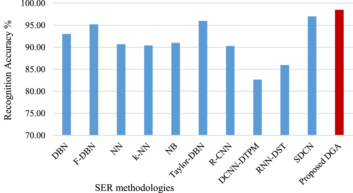
Comparative analysis of existing SER [17–19, 29, 41, 42] and proposed DGA framework.

5 Conclusion

Any classifier’s performance is degraded by emotion recognition with noisy signals. To overcome this problem, we propose a Deep Ganitrus Algorithm that automatically removes unnecessary noisy signals and recovers the crucial aspects from the augmented voice signal. The Deep Ganitrus is used to prepare the weights and bias for categorizing the specific emotions in the voice signal. Anger, joy, sadness, fear, disgust, boredom, and neutral are all recognized by DGA. The Berlin database is used to complete the simulation of the proposed method. Experimentation is conducted at various preparation rates. The conceptual inconsistencies of the precision, FAR, and FRR readings, respectively, are used to analyze the model’s reactions. The proposed system’s simulation result is compared with the performance of existing systems. As a result, it outperforms all other techniques in terms of recognition performance. Finally, we will explore several datasets to extract additional intriguing speech characteristics with improved emotion recognition accuracy in future research.

References

Bjekić

, Zlatić

and Bojović

, Students-teachers’communication competence: basic social communication skills andinteraction involvement, Journal of Educational Sciences &Psychology 10(1) (2020).

Bąk

Emotional Prosody Processing in Nonnative English Speakers. In Emotional Prosody Processing for Non-Native English Speakers (2016), 141–169, Springer, Cham.

Fishwick

P.A.

, Toward an integrative multimodeling interface: A human-computer interface approach to interrelating model structures, Simulation 80(9) (2004), 421–432.

Norman

Turn signals are the facial expressions of automobiles. Diversion Books (2014).

Adler

Understanding human nature: The psychology of personality. GENERAL PRESS (2020).

Edwards

N.E.

and Scheetz

P.S.

, Predictors of burden for cregivers of patients with Parkinson’s disease, Journal of Neuroscience Nursing 34(4) (2002), 184.

Shukla

, Jain

and Dubey

R.K.

, Increasing the performance of speech recognition system by using different optimization techniques to redesign artificial neural network, Journal of Theoretical and Applied Information Technology 97(8) (2019), 2404–2415.

Kerkeni

, Serrestou

, Mbarki

, Raoof

, Mahjoub

M.A.

, Cleder

Automatic speech emotion recognition using machine learning. In Social media and machine learning. IntechOpen (2019).

Jain

, Gupta

, Jain

N.K.

Analysis and design of digital IIR integrators and differentiators using minimax and pole, zero, and constant optimization methods, International Scholarly Research Notices (2013).

10.

Park

A.S.

and Glass

J.R.

, Unsupervised pattern discovery in speech, IEEE Transactions on Audio, Speech, and Language Processing 16(1) (2007), 186–197.

11.

Yogesh

C.K.

, Hariharan

, Ngadiran

, Adom

A.H.

, Yaacob

, Berkai

and Polat

, A new hybrid PSO assisted biogeography-based optimization for emotion and stress recognition from speech signal, Expert Systems with Applications 69 (2017), 149–158.

12.

Shukla

and Jain

, A novel system for effective speech recognition based on artificial neural network and opposition artificial bee colony algorithm, International Journal of Speech Technology 22 (4) (2019), 959–969.

13.

Huang

, Gong

, Fu

, Feng

A research of speech emotion recognition based on deep belief network and SVM, Mathematical Problems in Engineering (2014).

14.

Gupta

, Jain

and Kumar

, Novel class of stable wideband recursive digital integrators and differentiators, IET Signal Processing 4 (5) (2010), 560–566.

15.

Pustokhina

I.V.

, Pustokhin

D.A.

, Gupta

, Khanna

, Shankar

and Nguyen

G.N.

, An effective training scheme for deep neural network in edge computing enabled Internet of medical things (IoMT) systems, IEEE Access 8 (2020), 107112–107123.

16.

Jain

and Shukla

, Accurate speech emotion recognition by using brain-inspired decision-making spiking neural network, , International Journal of Advanced Computer Science and Applications 10 (2019), 12.

17.

Sun

T.W.

, End-to-end speech emotion recognition with gender information, 23, IEEE Access 8 (2020), 152423–152438.

18.

Zhang

, Zhang

, Huang

and Gao

, Speech emotion recognition using deep convolutional neural network and discriminant temporal pyramid matching, IEEE Transactions on Multimedia 20(6) (2017), 1576–1590.

19.

, Liu

, Yang

, Sun

and Wang

, Speech emotion recognition using recurrent neural networks with directional self-attention, , Expert Systems with Applications 173 (2021), 114683.

20.

Kwon

, A CNN-assisted enhanced audio signal processing for speech emotion recognition,, Sensors 20(1) (2020), 183.

21.

Vryzas

, Vrysis

, Matsiola

, Kotsakis

, Dimoulas

and Kalliris

, Continuous speech emotion recognition with convolutional neural networks, Journal of the Audio Engineering Society 68(1/2) (2020), 14–24.

22.

Sajjad

and Kwon

, Clustering-based speech emotion recognition by incorporating learned features and deep BiLSTM, 1–, IEEE Access 8 (2020), 79861–79875.

23.

Mohamed

M.M.

, Schuller

B.W.

Concealnet: An end-to-end neural network for packet loss concealment in deep speech emotion recognition. arXiv preprint arXiv:2005.07777 (2020).

24.

Chen

, Su

, Feng

, Wu

, She

and Hirota

, Two-layer fuzzy multiple random forest for speech emotion recognition in human-robot interaction, Information Sciences 509 (2020), 150–163.

25.

Mohamed

M.M.

, Schuller

B.W.

“I have vxxx bxx connexxxn!” Facing Packet Loss in Deep Speech Emotion Recognition. arXiv preprint arXiv:2005.07757 (2020).

26.

Zheng

, Wang

and Jia

, An ensemble model for multi-level speech emotion recognition, Applied Sciences 10(1) (2020), 205.

27.

Siriwardhana

, Reis

, Weerasekera

, Nanayakkara

Jointly Fine-Tuning” BERT-like” Self Supervised Models to Improve Multimodal Speech Emotion Recognition. arXiv preprint arXiv:2008.06682 (2020).

28.

Parthasarathy

and Busso

, Semi-supervised speech emotion recognition with ladder networks, IEEE/ACM Transactions on Audio, Speech, and Language Processing 28 (2020), 2697–2709.

29.

Shukla

and Jain

, A novel stochastic deep conviction network for emotion recognition in speech signal, Journal of Intelligent & Fuzzy Systems 38(4) (2020), 5175–5190.

30.

Hardainiyan

, Nandy

B.C.

and Kumar

, Elaeocarpus ganitrus(Rudraksha): A reservoir plant with their pharmacological effects, Int J Pharm Sci Rev Res 34(1) (2015), 55–64.

31.

Stone

J.V.

, Independent component analysis: an introduction, Trends in Cognitive Sciences 6(2) (2002), 59–64.

32.

Sun

, Fu

and Wang

, Decision tree SVM model with Fisher feature selection for speech emotion recognition, EURASIP Journal on Audio, Speech, and Music Processing 2019(1) (2019), 1–14.

33.

Wang

, Liu

C.L.

and Zheng

, August. Feature selection by combining Fisher criterion and principal feature analysis. In 2007 International Conference on Machine Learning and Cybernetics 2(2007), 1149–1154. IEEE.

34.

Carreira-Perpinan

M.A.

, Hinton

, January. On contrastive divergence learning. In International workshop on artificial intelligence and statistics (2005), 33–40. PMLR.

35.

Liu

J.W.

, Chi

G.H.

, Luo

X.L.

Contrastive divergence learning for the restricted Boltzmann machine. In 2013 Ninth International Conference on Natural Computation (ICNC) (2013), 18–22. IEEE.

36.

Wang

, An

, Li

B.N.

, Zhang

and Li

, Speech emotion recognition using Fourier parameters, IEEE Transactions on Affective Computing 6(1) (2015), 69–75.

37.

Hinton

G.E.

, Dayan

, Frey

B.J.

and Neal

R.M.

, The ”wake-sleep” algorithm for unsupervised neural networks, Science 268 (1995), 1158–1161.

38.

Bourez

Deep learning with Theano. Packt Publishing Ltd. (2017).

39.

Berlin database from http://emodb.bilderbar.info/docu/ Accessed May 2020.

40.

, Ayadi, M.S. Kamel and F. Karray, Survey on speech emotion recognition: Features, classification schemes, and databases, Pattern Recognition 44(3) (2011), 1158–587.

41.

Haridas

A.V.

, Marimuthu

, Sivakumar

V.G.

, Chakraborty

Emotion recognition of speech signal using Taylor series and deep belief network based classification, Evolutionary Intelligence (2020), 1–14.

42.

Mannepalli

, Sastry

P.N.

and Suman

, FDBN: Design and development of Fractional Deep Belief Networks for speaker emotion recognition, International Journal of Speech Technology 19(4) (2016), 779–790.

Deep ganitrus algorithm for speech emotion recognition

Abstract

Keywords

1 Introduction

2 Related works

3.2 Feature extraction: independent component analysis (ICA)

3.2.2 Pre-selection using fisher criterion

3.4 Restricted Boltzmann machines

4.1 Experimental setup

4.2 Dataset description

Table 3 EmoDB details S. No. No. of speakers Gender Age 1 03 M 31 2 08 F 34 3 09 F 21 4 10 M 32 5 11 M 26 6 12 M 30 7 13 F 32 8 14 F 35 9 15 M 25 10 16 F 31

Table 4 Hyperparameters and training statistics of the DGN Number of layers 5 Units per layer 50 Learning rate 0.01 Number of epochs 475 Recognition accuracy 0.985

References

Table 3
EmoDB details

S. No. No. of speakers Gender Age

1 03 M 31

2 08 F 34

3 09 F 21

4 10 M 32

5 11 M 26

6 12 M 30

7 13 F 32

8 14 F 35

9 15 M 25

10 16 F 31

Table 4
Hyperparameters and training statistics of the DGN

Number of layers 5

Units per layer 50

Learning rate 0.01

Number of epochs 475

Recognition accuracy 0.985