Numerical solution of bipolar fuzzy initial value problem

Abstract

Differential equations occur in many fields of science, engineering and social science as it is a natural way of modeling uncertain dynamical systems. A bipolar fuzzy set model is useful mathematical tool for addressing uncertainty which is an extension of fuzzy set model. In this paper, we study differential equations in bipolar fuzzy environment. We introduce the concept gH-derivative of bipolar fuzzy valued function. We present some properties of gH-differentiability of bipolar fuzzy valued function by considering different types of differentiability. We consider bipolar fuzzy Taylor expansion. By using Taylor expansion, Euler method is presented for solving bipolar fuzzy initial value problems. We discuss convergence analysis of proposed method. We describe some numerical examples to see the convergence and stability of the method and compute global truncation error. From numerical results, we see that for small step size Euler method converges to exact solution.

Keywords

Generalized Hukuhara derivative Bipolar Fuzzy Taylor expansion bipolar fuzzy initial value problem Euler method method convergence analysis 34A07

1 Introduction

Many problems of science and engineering are modeled in such a way that some of the information regarding the problems are incomplete, imprecise or vague. Fuzzy differential equations (DEs) arise in many dynamical systems. Zadeh [43] introduced the concept of fuzzy set to handle uncertainty which is due to vagueness or imprecision instead of randomness. Chang and Zadeh [13] introduced fuzzy numbers that are special types of fuzzy sets which satisfy certain conditions. They also introduced the fuzzy derivative. Following the approach of [13], extension principle has been used to define fuzzy derivative [14]. Puri and Ralescu [37] gave the notion of Hukara derivative of fuzzy valued function. Kaleva [26] studied the existence and uniqueness of the solution of fuzzy DEs. Seikkala [39] studied fuzzy initial value problems. Mondal and Roy [32] introduced a method to solve nonhomogeneous first order linear fuzzy DEs. Esfahani etal. [17] studied the existence and uniqueness of solutions of fuzzy boundary value problems. There are many fuzzy DEs whose analytic solutions do not exist or it is much difficult to handle analytically. For such differential equations, numerical procedures are often used. Ma etal. [31] used a numerical method to solve fuzzy IVPs based on standard Picard method. Error analysis of described method has been discussed. Abbasbandy and Allahviranloo [1] introduced Taylor method to solve fuzzy DEs. Effati and Pakdaman [15] used a novel approach for solving fuzzy IVPs based on neural network. They replaced the DE by a system of DEs and write the solution in two parts, one part satisfies the initial conditions and the other satisfies the feed-forward neural network that contain controllable parameters. Gisilov etal. [19] suggested a method based on linear transformation to solve high order linear DEs whose initial values are fuzzy. They presented the solution in the form of fuzzy functions that satisfy the initial value problem. Pederson and Sambandham [35] used Runge-Kutta method to find the solution of fuzzy DEs. A method based on Euler and improved Euler method introduced by Tapaswini and Chakraverty [41]. Fard and Gal [18] introduced an iterative method to resolve system of first order linear fuzzy DEs having fuzzy coefficients Parandin [34] applied RK-method to obtain numerical solution of n-th order fuzzy DEs. Tapaswini and Chakraverty [40,] introduced homotopy perturbation method and a method based on Euler method for fuzzy DEs. Jayakumar etal. [25] investigated and applied fifth order RK-method. Palligkinis etal. [33] utilized RK-method to solve more general fuzzy DEs and discussed the convergence analysis for s-stage RK-method. Ghazanfari etal. [20] applied a fourth order R-Kutta like method has used for numerical solution of fuzzy DEs. Ivaz etal. [23] developed algorithms to approximate the solution of first order fuzzy DEs and hybrid fuzzy DEs. Rabiei etal. [21] applied improved RK-nystrom method for second order fuzzy DEs. Characterization theorem has been used by Pederson and Sambandham [36] to obtain the numerical solution of fuzzy DEs. Allahviranloo et al. [5] introduced Adam-moulton, Adam-Bashforth and a predictor-corrector method in which three step Adam-Bashforth is used as predictor and two step Adam-Moulton method is used as corrector. Stability and convergence condition of proposed methods has been discussed. Several approaches have been used to solve fuzzy DEs based on H-derivatives. The first approach is due to Puri and Ralsue [37]. The major drawback of this approach is that the solution has increasing length of its support. Hullermeier [22] interpreted the fuzzy DE as system of differential inclusions. This approach has also a drawback that derivative of function does not present. Buckely and Feuring [10] described another approach based on Zadeh extension principle in which a crisp differential equation has been extended to fuzzy DE. This approach is based on differential inclusions. Buckely and Feuring [11] solved analytically nth-order linear differential equation with fuzzy initial conditions by two different approaches. In first approach, the crisp solution has been fuzzified to get fuzzy function and then it is checked whether this fuzzified function satisfies the differential equation or not. The second method is the reversal steps of first method. Many methods for solving fuzzy DEs based on system of crisp differential equations, that is fuzzy DE is converted to system of crisp DEs. Thus solving the system of crisp DE, we have the solution of fuzzy DE. It may be much difficult to manipulate complicated systems. Tapaswini etal. [42] proposed a method based on fuzzy radius and center to find the solution of n^th-order fuzzy differential equation. Two crisp differential equations are obtained in the form of fuzzy radius and center. Thus after having the fuzzy radius and center solution, the fuzzy solution can be obtained. Bade and Gal [9] gave the notion of strongly generalized differentiability and applied it to fuzzy DEs. Under this concept, the solution of fuzzy DE has decreasing length of its support. This concept is very useful in practical application as well as in theoretical evaluation of qualitative type [4]. Cano and Flores [12] introduced the notion of generalized H-differentiability. Lupulescu [30] gave the idea of inner product on fuzzy space to solve fuzzy IVPs. Jafari etal. [24] applied variational iteration method to solve n^th-order fuzzy DEs. Khastan and Lopez [27] studied different formulation of first order linear fuzzy DEs with generalized differentiability. They obtained a general form of these solutions that show different behaviors.

Sometimes, we have the information that have two poles, one for satisfaction and other for dissatisfaction. Coexistence, harmony and equilibrium between two sides can be regarded as an essential to human being’s intellectual and materialistic health and to the strength and success of social system. Zhang [47, 48] enlarged the concept of fuzzy set to bipolar fuzzy set. The structure of bipolar fuzzy set and intuitionistic fuzzy set look very much like to each other but Lee [29] has pointed out some essential distinction between bipolar fuzzy sets and intuitionistic fuzzy sets. Lee [28] studied some basic operations of bipolar fuzzy sets. The bipolar fuzzy frame has more attraction for researchers as compared to fuzzy frame. A bipolar fuzzy has positive and negative parts. The positive part shows the possibility and negative part shows the impossibility. Akram and Arshad [2] introduced a new method for group decision making. Recently, Akram etal. [3] extended the fuzzy system of linear equations to bipolar fuzzy system of linear equations and resolved this system for (-1,1)-cut. The rest of the paper is structured as follows: In section 2, we give some definitions and basic results. Some properties of gH-differentiability are given in section 3. In section 4, we demonstrate Taylor theorem for bipolar fuzzy valued functions. In section 5, we describe bipolar fuzzy initial value problem and some related theorems. We present Euler method for bipolar fuzzy IVPs in section 6. Consistency, stability and convergence of proposed method have been discussed in section 7. In section 8, a few numerical examples have been presented. Lastly, we draw some conclusions in section 9.

2 Preliminaries

We provide necessary notions and results that would be used in the sequel.

Definition 2.1. [48] Let $X$ be a nonempty set, a bipolar fuzzy set $A$ is an object of the form $\begin{matrix} A = {< x, μ_{A}^{P} (x), μ_{A}^{N} (x) > | x \in X}, \end{matrix}$ which is characterized by satisfaction degree of a certain property $μ_{A}^{P}$ and satisfaction of its counter property $μ_{A}^{N}$ , where $μ_{A}^{P} : X ⟶ [0, 1]$ and $μ_{A}^{N} : X ⟶ [- 1, 0]$ .

Definition 2.2. [2] Let $A$ be bipolar fuzzy number and α ∈ [0, 1] andβ ∈ [-1, 0], the (α, β)-cut of $A$ is defined as: $\begin{matrix} A^{(α, β)} = {x \in R | μ_{A}^{P} (x) \geq α, μ_{A}^{N} (x) \leq β} . \end{matrix}$

Lemma 2.3. For any bipolar fuzzy set $A$ , $[A]^{(α, β)}$ is convex if and only if $μ_{A}^{P}$ and $μ_{A}^{N}$ are convex and concave, respectively.

Proof. Let $[A]^{(α, β)}$ be convex and $x, y \in [A]^{(α, β)}$ . Let $min {μ_{A}^{P} (x), μ_{A}^{P} (y)} = ξ \geq α$ and $max {μ_{A}^{N} (x), μ_{A}^{N} (y)} = η \leq β$ For any $x, y \in [A]^{(ξ, η)}$ and δ ∈ [0, 1], we have $δ x + (1 - δ) y \in [A]^{(ξ, η)}$ , $\begin{matrix} \Rightarrow μ_{A}^{P} (δ x + (1 - δ) y) \geq ξ and μ_{A}^{N} (δ x + (1 - δ) y) \leq η . \end{matrix}$ $\begin{matrix} \begin{matrix} Thus, μ_{A}^{P} (δ x + (1 - δ) y) \geq min {μ_{A}^{P} (x), μ_{A}^{P} (y)} \\ and μ_{A}^{N} (δ x + (1 - δ) y) \leq max {μ_{A}^{N} (x), μ_{A}^{N} (y)} . \end{matrix} \end{matrix}$ Hence $μ_{A}^{P}$ and $μ_{A}^{N}$ are convex and concave, respectively.

Conversely, let $μ_{A}^{P}$ and $μ_{A}^{N}$ are convex and concave, respectively, and $x, y \in [A]^{(α, β)}, for α \in [0, 1] and β \in [- 1, 0],$ we have $\begin{matrix} μ_{A}^{P} (x) \geq α, μ_{A}^{P} (y) \geq α and μ_{A}^{N} (x) \leq β, μ_{A}^{N} (y) \leq β . \end{matrix}$ Since, $μ_{A}^{P}$ and $μ_{A}^{N}$ are convex and concave, respectively, for δ ∈ [0, 1], we have $\begin{matrix} \begin{matrix} μ_{A}^{P} (δ x + (1 - δ) y) \geq min {μ_{A}^{P} (x), μ_{A}^{P} (y)} and \\ μ_{A}^{N} (δ x + (1 - δ) y) \leq max {μ_{A}^{N} (x), μ_{A}^{N} (y)} . \end{matrix} \end{matrix}$ Thus, $\begin{matrix} δ x + (1 - δ) y \in [A]^{(α, β)}, \forall x, y \in [A]^{(α, β)}, δ \in [0, 1] . \end{matrix}$ □

Definition 2.4. [3] The parametric form of BFN $u$ is a quadruple $≺ [{\underline{u}}^{P}, {\bar{u}}^{P}], [{\underline{u}}^{N}, {\bar{u}}^{N}] ≻$ of the functions ${\underline{u}}^{P} (t), {\bar{u}}^{P} (t), {\underline{u}}^{N} (w), {\bar{u}}^{N} (w)$ ; 0 ≤ t ≤ 1, -1 ≤ w ≤ 0 which satisfy the following conditions:

${\underline{u}}^{P} (t)$ is a bounded, non-decreasing, right continuous at 0 and left continuous function on (0, 1].

${\bar{u}}^{P} (t)$ is a bounded, non-increasing, right continuous at 0 and left continuous function on (0, 1].

${\underline{u}}^{N} (w)$ is a bounded, non-increasing, right continuous at ’-1’ and left continuous function on (-1, 0].

${\bar{u}}^{N} (w)$ is a bounded, non-decreasing, right continuous at ’-1’ and left continuous function on (-1, 0].

${\underline{u}}^{P} (t) \leq {\bar{u}}^{P} (t)$ .

${\underline{u}}^{N} (w) \leq {\bar{u}}^{N} (w)$ .

Definition 2.5. [3] For any $u = ≺ [\underline{u^{P}} (t), {\bar{u}}^{P} (t)]$ , $[{\underline{u}}^{N} (w), {\bar{u}}^{N} (w)] ≻$ , $v = ≺ [{\underline{v}}^{P} (t), {\bar{v}}^{P} (t)]$ , $[{\underline{v}}^{N} (w), {\bar{v}}^{N} (w)] ≻$ and $c \in ℝ$ ; 0 ≤ t ≤ 1, -1≤ w ≤ 0, the addition and multiplication are laid out as;

$(\underline{u^{P} \oplus v^{P}}) (t) = {\underline{u}}^{P} (t) + {\underline{v}}^{P} (t)$ , $(\bar{u^{P} \oplus v^{P}}) (t) = {\bar{u}}^{P} (t) + {\bar{v}}^{P} (t)$ ,

$(\underline{u^{N} \oplus v^{N}}) (w) = {\underline{u}}^{N} (w) + {\underline{v}}^{N} (w)$ , $(\bar{u^{N} \oplus v^{N}}) (w) = {\bar{u}}^{N} (w) + {\bar{v}}^{N} (w)$ ,

${\underline{u^{P} ⊙ v}}^{P} = min {{\underline{u}}^{P} {\underline{v}}^{P}, {\underline{u}}^{P} {\bar{v}}^{P}, {\bar{u}}^{P} {\underline{v}}^{P}, {\bar{u}}^{P} {\bar{v}}^{P}}$ ,

$\bar{u^{P} ⊙ v^{P}} = max {{\underline{u}}^{P} {\underline{v}}^{P}, {\underline{u}}^{P} {\bar{v}}^{P}, {\bar{u}}^{P} {\underline{v}}^{P}, {\bar{u}}^{P} {\bar{v}}^{P}}$ ,

${\underline{u^{N} ⊙ v}}^{N} = max {{\underline{u}}^{N} {\underline{v}}^{N}, {\underline{u}}^{N} {\bar{v}}^{N}, {\bar{u}}^{N} {\underline{v}}^{N}, {\bar{u}}^{N} {\bar{v}}^{N}}$ ,

$\bar{u^{N} ⊙ v^{N}} = min {{\underline{u}}^{N} {\underline{v}}^{N}, {\underline{u}}^{N} {\bar{v}}^{N}, {\bar{u}}^{N} {\underline{v}}^{N}, {\bar{u}}^{N} {\bar{v}}^{N}}$ ,

For c ≥ 0, $({\underline{c ⊙ u}}^{P}) (t) = c ({\underline{u}}^{P}) (t)$ , $({\bar{c ⊙ u}}^{P}) (t) = c ({\bar{u}}^{P}) (t)$ , $({\underline{c ⊙ u}}^{N}) (w) = c ({\underline{u}}^{N}) (w)$ , $({\bar{c ⊙ u}}^{N})$ $(w) = c ({\bar{u}}^{N}) (w)$ ,

Forc < 0, $({\underline{c ⊙ u}}^{P}) (t) = c ({\bar{u}}^{P}) (t)$ , $({\bar{c ⊙ u}}^{P}) (t) = c ({\underline{u}}^{P}) (t)$ , $({\underline{c ⊙ u}}^{N}) (w) = c ({\bar{u}}^{N}) (w)$ , $({\bar{c ⊙ u}}^{N}) (w) = c ({\underline{u}}^{N}) (w)$ .

The space of all bipolar fuzzy numbers is denoted by $B_{F}$ .

Theorem 2.6. If $u \in B_{F}$ , then;

$[u]^{α}, [u]^{β} \in P_{K} (ℝ), \forall 0 \leq α \leq 1, - 1 \leq β \leq 0,$ where $P_{K} (ℝ)$ is the space of convex and compact subsets of $ℝ$ .

[u] ^α
₂ ⊆ [u] ^α
₁and [u] ^β
₂ ⊆ [u] ^(β₁), for0 ≤ α₁ ≤ α₂ ≤ 1, and - 1 ≤ β₂ ≤ β₁ ≤ 0.

Further, if (α_k) is non-decreasing sequence converging to α > 0 and (β_k) is non-increasing sequence converging to β > -1, then

[u] ^α = ⋂ _k≥1 [u] ^α
_kand [u] ^β = ⋂ _k≥1 [u] ^β
_k .

Conversely, if

A^{α} = {x \in ℝ : 0 \leq α \leq 1}

and

B^{β} = {y \in ℝ : - 1 \leq β \leq 0}

be two families of subsets of

ℝ

satisfying conditions (i)-(iii), then there is a

u \in B_{F}

such that

\begin{matrix} \begin{matrix} [u]^{α} & = A^{α}, for 0 < α \leq 1 and [u]^{β} = B^{β}, for \\ - 1 \leq β < 0 . \end{matrix} \end{matrix}

Proof. Let $u \in B_{F}$ , then for 0 ≤ α₁ ≤ α₂ ≤ 1, we have [u] ^{α
₂} ⊆ [u] ^{α
₁} ⊆ [u] ⁰, where [u] ⁰ = cl ⋃ _α∈(0,1] [u] ^α.

Also for -1 ≤ β₁ ≤ β₂ ≤ 0, we have [u] ^{β
₁} ⊆ [u] ^{β
₂} ⊆ [u] ⁰, where [u] ⁰ = cl ⋃ _β∈[-1,0) [u] ^β.

Since, u is normal, that is, there exist $x, y \in ℝ$ such that u^P (x) =1 and u^N (y) = -1, u^P maps $ℝ$ onto [0, 1] and u^N maps $ℝ$ onto [-1, 0].

Also, [u] ^α and [u] ^β are convex subsets of $ℝ$ , for all α ∈ [0, 1] andβ ∈ [-1, 0]. For any nondecreasing sequence (α_i) converging to α ∈ [0, 1] and non-increasing sequence (β_i) converging to β ∈ [-1, 0], we have [u] ^α = ⋂ _k≥1 [u] ^{a
_k}and [u] ^β = ⋂ _k≥1 [u] ^{β
_k} .

To prove converse, let x ∈ A⁰, define I_x = [α ∈ [0, 1] : x ∈ A^α] and let α₀ = supI_x. We claim that I_x = [0, α₀]. If α₀ = 0, then there is nothing to prove. Suppose α > 0 and let α₁ ∈ (0, α₀), then there exists α₂ ∈ [α₁, α₀) such that α₂ ∈ I_x. Thus, x ∈ A^{α
₂}, by (ii), x ∈ A^{α
₁} and α₁ ∈ I_x. Also 0 ∈ I_x, hence [0, α₀) ⊆ I_x. As (α_i) is nondecreasing sequence converging to α₀ in I_x. So, x ∈ A^{α
_i} for each i = 1, 2, ⋯ and therefore, by (iii), x ∈ A^{α
₀}. Thus, α₀ ∈ I_x, and [0, α₀] ⊆ I_x.

Again, α₁ ∈ I_x implies that α₁ ≤ α₀, we have I_x ⊆ [0, α₀]. Hence, I_x = [0, α₀].

Let α ∈ [0, 1], if x ∈ [u] ^α, then u (x) ≥ α > 0 and so, x ∈ A⁰ and $u (x) = \underset{x}{supI} = α_{0} \geq α$ . Hence, x ∈ A⁰ and by (ii), x ∈ A^α thus, [u] ^α ⊆ A^α.

Conversely, if x ∈ A^α, then $u (x) = \underset{x}{supI} = α_{0} \geq α$ and thus, x ∈ [u] ^α. This implies A^α ⊆ [u] ^α. Combining the results, we obtain [u] ^α = A^α. Let y ∈ B⁰, define I_y = [α ∈ [-1, 0] : y ∈ B^β] and let $β_{0} = \underset{y}{infI}$ . We claim that I_y = [β₀, 0]. If β₀ = 0, then there is nothing to prove. Suppose β < 0 and let, β₁ ∈ (β₀, 0), then there exists β₂ ∈ [β₀, β₁) such that β₂ ∈ I_y. Thus, y ∈ B^{β
₂}, by (ii), y ∈ B^{β
₁} and β₁ ∈ I_y. Also, 0 ∈ I_y, hence (β₀, 0]) ⊆ I_y. As, (β_i) is non-increasing sequence converging to β₀ in I_y. So, y ∈ B^{β
_i} for each i = 1, 2, ⋯ and therefore, by (iii), y ∈ B^{β
₀}. Thus, β₀ ∈ I_y, hence, [β₀, 0] ⊆ I_y.

Again, β₁ ∈ I_y implies that β₀ ≤ β₁, we have I_y ⊆ [β₀, 0]. Hence, I_y = [β₀, 0].

Let, β ∈ [-1, 0], if y ∈ [u] ^β, then u (y) ≤ β < 0 and so, y ∈ B⁰ and $u (y) = \underset{y}{infI} = β_{0} \leq β$ . Hence, y ∈ B⁰ and by (ii), y ∈ A^β thus, [u] ^β ⊆ A^β. Conversely, if y ∈ B^β, then $u (y) = \underset{y}{infI} = β_{0} \leq β$ and thus, y ∈ [u] ^β. This implies A^β ⊆ [u] ^β. Combining the results, we obtain [u] ^β = A^β.

We find that u^P maps $ℝ$ onto [0, 1] and u^N maps $ℝ$ onto [-1, 0], so u maps $ℝ$ onto [0, 1] × [-1, 0]. Also since [u] ^α and [u] ^β are convex, so, by Lemma 2.20, u^P and u^N are fuzzy convex and concave respectively. Hence, $u \in B_{F}$ . □

Definition 2.7. Let $u = ≺ [{\underline{u}}^{P} (r), {\bar{u}}^{P} (r)]$ , $[{\underline{u}}^{N} (s), {\bar{u}}^{N} (s)] ≻ \in B_{F}$ , then length of $u$ is

$\begin{matrix} diam (u) = max {max_{0 \leq r \leq 1} | {\bar{u}}^{P} (r) - {\bar{u}}^{P} (r) |, \\ max_{- 1 \leq s \leq 0} | {\bar{u}}^{N} (s) - {\underline{u}}^{N} (s) |} \end{matrix}$

Definition 2.8. The generalized H-difference of two bipolar fuzzy numbers $u, v \in B_{F}$ is defined as $\begin{matrix} u \underset{gH}{⊖} v = w \Leftrightarrow {\begin{matrix} (a) u = v \oplus w, \\ (b) v = u \oplus (- 1) w . \end{matrix} \end{matrix}$ $u \underset{gH}{⊖} v$ exists if and only if $u^{P} \underset{gH}{⊖} v^{P}$ and $u^{N} \underset{gH}{⊖} v^{N}$ both exist. That is,

$\begin{matrix} u^{P} \underset{gH}{⊖} v^{P} = w^{P} \Leftrightarrow {\begin{matrix} (a_{1}) u^{P} = v^{P} \oplus w^{P}, \\ (b_{1}) v^{P} = u^{P} \oplus (- 1) w^{P} . \end{matrix} \end{matrix}$ and $\begin{matrix} u^{N} \underset{gH}{⊖} v^{N} = w^{N} \Leftrightarrow {\begin{matrix} (a_{2}) u^{N} = v^{N} \oplus w^{N}, \\ (b_{2}) v^{N} = u^{N} \oplus (- 1) w^{N} . \end{matrix} \end{matrix}$

Definition 2.9. Let $u = ≺ [{\underline{u}}^{P} (r), {\bar{u}}^{P} (r)]$ , $[{\underline{u}}^{N} (s), {\bar{u}}^{N} (s)] ≻$ and $v = ≺ [{\underline{v}}^{P} (r), {\bar{v}}^{P} (r)], [{\underline{v}}^{N} (s), {\bar{v}}^{N} (s)] ≻$ , we define metric $D : B_{F} \times B_{F} \to ℝ^{+} \cup {0}$ as follows; $\begin{matrix} D (u, v) = max [max_{0 \leq r \leq 1} {| {\underline{u}}^{P} (r) - {\underline{v}}^{P} (r) |, | {\bar{u}}^{P} (r) - {\bar{v}}^{P} (r) |}, \\ \max_{- 1 \leq s \leq 0} {| {\underline{u}}^{N} (s) - {\underline{v}}^{N} (s) |, | {\bar{u}}^{N} (s) - {\bar{u}}^{N} (s) |}] . \end{matrix}$ That is, if $D_{1} (u^{P}, v^{P}) = max_{0 \leq r \leq 1} {| {\underline{u}}^{P} (r) - {\underline{v}}^{P} (r) |, | {\bar{u}}^{P} (r) - {\bar{v}}^{P} (r) |}$ and $D_{2} (u^{N}, v^{N}) = max_{- 1 \leq s \leq 0} {| {\underline{u}}^{N} (s) - {\underline{v}}^{N} (s) |, | {\bar{u}}^{N} (s) - {\bar{u}}^{N} (s) |}$ , are two metric spaces then $D (u, v) = max (D_{1} (u^{P}, v^{P}), D_{2} (u^{N}, v^{N}))$ .

It is easy to see that $D$ satisfies the following properties;

$D (u oplus w, v oplus w) = D (u, v)$ , $\forall u, v, w \in B_{F}$ .

$D (λ ⨀ u, λ ⨀ v) = | λ | D (u, v)$ , $\forall u, v \in B_{F}, λ \in ℝ$ .

$D (u oplus v, w oplus e) \leq D (u, w) + D (v, e)$ , $\forall u, v, w, e \in B_{F}$ .

$D (u ⊖ v, w ⊖ e) \leq D (u, w) + D (v, e)$ , when $u ⊖ v$ and $w ⊖ e$ both exist, $\forall u, v, w, e \in B_{F}$ .

Where ⊖ is H-difference, that is

u ⊖ v = w

if and only if

u = v \oplus w

(v). $(B_{F}, D)$ is a complete metric space.

Definition 2.10. A bipolar fuzzy valued function $F : J \to B_{F}$ is called continuous at t₀ ∈ J if for any ε > 0, there exists a δ > 0 such that $D (F (t), F (t_{0})) < ε$ , whenever |t - t₀| < δ. If $F$ is continuous at each point of J then it is continuous on J.

$F$ is continuous if and only if both $F^{P}$ and $F^{N}$ are continuous.

Definition 2.11. Let $F : J \to B_{F}$ and t₀ ∈ J, then $F$ is gH-differentiable at t₀ ∈ J if there is $F^{'} (t_{0}) \in B_{F}$ such that $lim_{k \to 0^{+}} \frac{F (t_{0} + k) ⊖_{gH} F (t_{0})}{k}$ exist and equal to $F^{'} (t_{0})$ .

Definition 2.12. A bipolar fuzzy valued function $F : I \to B_{F}$ is said to be

[i - gH]-differentiable if for k > 0, the differences $F^{P} (t_{0} + k) \underset{gH}{⊖} F^{P} (t_{0})$ and $F^{N} (t_{0} + k) \underset{gH}{⊖} F^{N} (t_{0})$ exist as case (a₁) and (a₂) of Definition 2.8, respectively, and limits $lim_{k \to 0^{+}} \frac{F^{P} (t_{0} + k) ⊖_{gH} F^{P} (t_{0})}{k}$ and $lim_{k \to 0^{+}} \frac{F^{N} (t_{0} + k) ⊖_{gH} F^{N} (t_{0})}{k}$ exist and equal to $F_{i . gH}^{' P} (t_{0})$ and $F_{i . gH}^{' N} (t_{0})$ , respectively.

[(i, ii) - gH]-differentiable if for k > 0, the differences $F^{P} (t_{0} + k) \underset{gH}{⊖} F^{P} (t_{0})$ and $F^{N} (t_{0} + k) \underset{gH}{⊖} F^{N} (t_{0})$ exist as case (a₁) and (b₂) of Definition 2.8, respectively, and limits $lim_{k \to 0^{+}} \frac{F^{P} (t_{0} + k) ⊖_{gH} F^{P} (t_{0})}{k}$ and $lim_{k \to 0^{+}} \frac{F^{N} (t_{0} + k) ⊖_{gH} F^{N} (t_{0})}{k}$ exist and equal to $F_{i . gH}^{' P} (t_{0})$ and $F_{ii . gH}^{' N} (t_{0})$ , respectively.

[(ii, i) - gH]-differentiable if for k > 0, the differences $F^{P} (t_{0} + k) \underset{gH}{⊖} F^{P} (t_{0})$ and $F^{N} (t_{0} + k) \underset{gH}{⊖} F^{N} (t_{0})$ exist as case (a₂) and (b₁) of Definition 2.8, respectively, and limits $lim_{k \to 0^{+}} \frac{F^{P} (t_{0} + k) ⊖_{gH} F^{P} (t_{0})}{k}$ and $lim_{k \to 0^{+}}$ $\frac{F^{N} (t_{0} + k) ⊖_{gH} F^{N} (t_{0})}{k}$ exist and equal to $F_{ii . gH}^{' P} (t_{0})$ and $F_{i . gH}^{' N} (t_{0})$ , respectively.

[ii - gH]-differentiable if for k > 0, the differences $F^{P} (t_{0} + k) \underset{gH}{⊖} F^{P} (t_{0})$ and $F^{N} (t_{0} + k) \underset{gH}{⊖} F^{N} (t_{0})$ exist as case (a₂) and (b₂) of Definition 2.8, respectively, and limits $lim_{k \to 0^{+}} \frac{F^{P} (t_{0} + k) ⊖_{gH} F^{P} (t_{0})}{k}$ and $lim_{k \to 0^{+}}$ $\frac{F^{N} (t_{0} + k) ⊖_{gH} F^{N} (t_{0})}{k}$ exist and equal to $F_{ii . gH}^{' P} (t_{0})$ and $F_{ii . gH}^{' P} (t_{0})$ , respectively.

Definition 2.13. Let $F : J \to B_{F}$ be bipolar fuzzy valued function then (α, β)-cut of F is given by $\begin{matrix} \begin{matrix} [F (t)]^{(α, β)} = ≺ [{\underline{F}}^{P} (t; α), {\bar{F}}^{P} (t; α)], \\ [{\underline{F}}^{N} (t; β), {\bar{F}}^{N} (t; β)] ≻, \end{matrix} \end{matrix}$ where $\begin{matrix} {\underline{F}}^{P} (t; α) & = min {F^{P} (t; α) : t \in J, 0 \leq α \leq 1}, \\ {\bar{F}}^{P} (t; α) & = max {F^{P} (t; α) : t \in J, 0 \leq α \leq 1}, \\ {\underline{F}}^{N} (t; β) & = min {F^{N} (t; β) : t \in J, - 1 \leq β \leq 0}, \\ {\bar{F}}^{N} (t; β) & = max {F^{N} (t; β) : t \in J, - 1 \leq β \leq 0}, \end{matrix}$ and ${\underline{F}}^{P} (t; α) \leq {\bar{F}}^{P} (t; α)$ , ${\underline{F}}^{N} (t; β) \leq {\bar{F}}^{N} (t; β)$ .

Theorem 2.14. Let $F : J \to B_{F}$ and $[F (t)]^{(α, β)} = ≺ [{\underline{F}}^{P} (t; α), {\bar{F}}^{P} (t; α)], [{\underline{F}}^{N} (t; β), {\bar{F}}^{N} (t; β)] ≻$ , for each α ∈ [0, 1] and β ∈ [-1, 0],

If $F$ is [i - gH]-differentiable then ${\underline{F}}_{α}^{P}, {\bar{F}}_{α}^{P}, {\underline{F}}_{β}^{N}, and {\bar{F}}_{β}^{N}$ all are differentiable and ${\underline{F^{'}}}^{P} (t; α) \leq {\bar{F^{'}}}^{P} (t; α)$ , ${\underline{F^{'}}}^{N} (t; β) \leq {\bar{F^{'}}}^{N} (t; β)$ and

$\begin{matrix} [F^{'} (t)]^{(α, β)} = ≺ [{\underline{F^{'}}}^{P} (t; α), {\bar{F^{'}}}^{P} (t; α)], \\ [{\underline{F^{'}}}^{N} (t; β), {\bar{F^{'}}}^{N} (t; β)] ≻ . \end{matrix}$ (1)

If $F$ is [(i, ii) - gH]-differentiable then ${\underline{F}}_{α}^{P}, {\bar{F}}_{α}^{P}, {\underline{F}}_{β}^{N}, and {\bar{F}}_{β}^{N}$ all are differentiable and ${\underline{F^{'}}}^{P} (t; α) \leq {\bar{F^{'}}}^{P} (t; α)$ , ${\bar{F^{'}}}^{N} (t; β) \leq {\underline{F^{'}}}^{N} (t; β)$ and

$\begin{matrix} [F^{'} (t)]^{(α, β)} = ≺ [{\underline{F^{'}}}^{P} (t; α), {\bar{F^{'}}}^{P} (t; α)], \\ [{\bar{F^{'}}}^{N} (t; β), {\underline{F^{'}}}^{N} (t; β)] ≻ . \end{matrix}$ (2)

If $F$ is [(ii, i) - gH]-differentiable then ${\bar{F}}_{α}^{P}, {\underline{F}}_{α}^{P}, {\underline{F}}_{β}^{N}, and {\bar{F}}_{β}^{N}$ all are differentiable and ${\bar{F^{'}}}^{P} (t; α) \leq {\underline{F^{'}}}^{P} (t; α)$ , ${\underline{F^{'}}}^{N} (t; β) \leq {\bar{F^{'}}}^{N} (t; β)$ and

$\begin{matrix} [F^{'} (t)]^{(α, β)} = ≺ [{\bar{F^{'}}}^{P} (t; α), {\underline{F^{'}}}^{P} (t; α)], \\ [{\underline{F^{'}}}^{N} (t; β), {\bar{F^{'}}}^{N} (t; β)] ≻ . \end{matrix}$ (3)

If $F$ is [ii - gH]-differentiable then ${\underline{F}}_{α}^{P}, {\bar{F}}_{α}^{P}, {\underline{F}}_{β}^{N}, and {\bar{F}}_{β}^{N}$ all are differentiable and ${\bar{F^{'}}}^{P} (t; α) \leq {\underline{F^{'}}}^{P} (t; α)$ , ${\bar{F^{'}}}^{N} (t; β) \leq {\underline{F^{'}}}^{N} (t; β)$ and

$\begin{matrix} [F^{'} (t)]^{(α, β)} = ≺ [{\bar{F^{'}}}^{P} (t; α), {\underline{F^{'}}}^{P} (t; α)], \\ [{\bar{F^{'}}}^{N} (t; β), {\underline{F^{'}}}^{N} (t; β)] ≻ . \end{matrix}$ (4)

Proof. (1) If k > 0, α ∈ [0, 1], β ∈ [-1, 0], $F^{P} (t + k) \underset{gH}{⊖} F^{P} (t)$ exists as in case (a₁) and $F^{N} (t + k) \underset{gH}{⊖} F^{N} (t)$ exists as in (a₂), then we have $\begin{matrix} [F (t + k) \underset{gH}{⊖} F (t)]^{(α, β)} = \\ ≺ [{\underline{F}}_{α}^{P} (t + k) - {\underline{F}}_{α}^{P} (t), {\bar{F}}_{α}^{P} (t + k) - {\bar{F}}_{α}^{P} (t)], \\ [{\underline{F}}_{β}^{N} (t + k) - {\underline{F}}_{β}^{N} (t), {\bar{F}}_{β}^{N} (t + k) - {\bar{F}}_{β}^{N} (t)] ≻ \end{matrix}$ Multiplying by $\frac{1}{k}$ $\begin{matrix} \frac{[F (t + k) ⊖_{gH} F (t)]^{(α, β)}}{k} = \\ ≺ [\frac{{\underline{F}}_{α}^{P} (t + k) - {\underline{F}}_{α}^{P} (t)}{k}, \frac{{\bar{F}}_{α}^{P} (t + k) - {\bar{F}}_{α}^{P} (t)}{k}], \\ [\frac{{\underline{F}}_{β}^{N} (t + k) - {\underline{F}}_{β}^{N} (t)}{k}, \frac{{\bar{F}}_{β}^{N} (t + k) - {\bar{F}}_{β}^{N} (t)}{k}] ≻ . \end{matrix}$ Similarly, $\begin{matrix} \frac{[F (t) ⊖_{gH} F (t - k)]^{(α, β)}}{k} = \\ ≺ [\frac{{\underline{F}}_{α}^{P} (t) - {\underline{F}}_{α}^{P} (t - k)}{h}, \frac{{\bar{F}}_{α}^{P} (t) - {\bar{F}}_{α}^{P} (t - k)}{k}], \\ [\frac{{\underline{F}}_{β}^{N} (t) - {\underline{F}}_{β}^{N} (t - k)}{k}, \frac{{\bar{F}}_{β}^{N} (t) - {\bar{F}}_{β}^{N} (t - k)}{k}] ≻ . \end{matrix}$ Taking limit k → 0, we have $\begin{matrix} [F^{'} (t)]^{(α, β)} = ≺ [{\underline{F^{'}}}^{P} (t; α), {\bar{F^{'}}}^{P} (t; α)], \\ [{\underline{F^{'}}}^{N} (t; β), {\bar{F^{'}}}^{N} (t; β)] ≻ . \end{matrix}$ (2) If k > 0, α ∈ [0, 1], β ∈ [-1, 0], $F^{P} (t + k) \underset{gH}{⊖} F^{P} (t)$ exists as in case (a₁) and $F^{N} (t + k) \underset{gH}{⊖} F^{N} (t)$ exists as in (b₂), then we have $\begin{matrix} [F (t + k) \underset{gH}{⊖} F (t)]^{(α, β)} = \\ ≺ [{\underline{F}}_{α}^{P} (t + k) - {\underline{v}}_{α}^{P} (t), {\bar{F}}_{α}^{P} (t + k) - {\bar{F}}_{α}^{P} (t)], \\ [{\bar{F}}_{β}^{N} (t + k) - {\bar{F}}_{β}^{N} (t), {\underline{F}}_{β}^{N} (t + k) - {\underline{F}}_{β}^{N} (t)] ≻ \end{matrix}$ Multiplying by $\frac{1}{k}$ $\begin{matrix} \frac{[F (t + k) ⊖_{gH} F (t)]^{(α, β)}}{k} = \\ ≺ [\frac{{\bar{F}}_{α}^{P} (t + k) - {\bar{F}}_{α}^{P} (t)}{k}, \frac{{\underline{F}}_{α}^{P} (t + k) - {\underline{F}}_{α}^{P} (t)}{k}], \\ [\frac{{\bar{F}}_{β}^{N} (t + k) - {\bar{F}}_{β}^{N} (t)}{k}, \frac{{\underline{F}}_{β}^{N} (t + k) - {\underline{F}}_{β}^{N} (t)}{k}] ≻ . \end{matrix}$ Similarly, $\begin{matrix} \frac{[F (t) ⊖_{gH} F (t - k)]^{(α, β)}}{k} = \\ ≺ [\frac{{\bar{F}}_{α}^{P} (t) - {\bar{F}}_{α}^{P} (t - k)}{k}, \frac{{\underline{F}}_{α}^{P} (t) - {\underline{F}}_{α}^{P} (t - k)}{k}], \\ [\frac{{\bar{F}}_{β}^{N} (t) - {\bar{F}}_{β}^{N} (t - k)}{k}, \frac{{\underline{F}}_{β}^{N} (t) - {\underline{F}}_{β}^{N} (t - k)}{k}] ≻ . \end{matrix}$ Taking limit k → 0, we have $\begin{matrix} [F^{'} (t)]^{(α, β)} = ≺ [{\underline{F^{'}}}^{P} (t; α), {\bar{F^{'}}}^{P} (t; α)], [{\bar{F^{'}}}^{N} (t; β), \\ {\underline{F^{'}}}^{N} (t; β)] ≻ . \end{matrix}$ □

In similar manners, we can prove (3) and (4).

Definition 2.15. A point t₀ ∈ J is called a switching point for differentiability of the function $F$ if in any neighborhood $U$ of t₀, there are points t₁ < t₀ < t₂ such that

Type (I) At t = t₁, it is [i - gH]-differentiable and at t = t₂ it is [(ii, i) - gH]-differentiable, or

Type (II) At t = t₁, it is [(ii, i) - gH]-differentiable and at t = t₂, it is [i - gH]-differentiable, or

Type (III) At t = t₁, it is [(i, ii) - gH]-differentiable and at t = t₂, it is [ii - gH]-differentiable, or

Type (IV) At t = t₁ it is [ii - gH]-differentiable and at t = t₂, it is [(i, ii) - gH]-differentiable, or

Type (V) At t = t₁, it is [i - gH]-differentiable and at t = t₂, it is [(i, ii) - gH]-differentiable, or

Type (VI) At t = t₁, it is [(i, ii) - gH]-differentiable and at t = t₂, it is [i - gH]-differentiable, or

Type (VII) At t = t₁, it is [(ii, i) - gH]-differentiable and at t = t₂, it is [ii - gH]-differentiable, or

Type (VIII) At t = t₁, it is [ii - gH]-differentiable and at t = t₂, it is [(ii, i) - gH]-differentiable, or

Type (IX) At t = t₁, it is [i - gH]-differentiable and at t = t₂, it is [ii - gH]-differentiable, or

Type (X)At t = t₁, it is [ii - gH]-differentiable and at t = t₂, it is [i - gH]-differentiable, or

Type (XI)At t = t₁, it is [(i, ii) - gH]-differentiable and at t = t₂, it is [(ii, i) - gH]-differentiable, or

Type (XII)At t = t₁, it is [(ii, i) - gH]-differentiable and at t = t₂, it is [(i, ii) - gH]-differentiable.

Definition 2.16. Let $F : (a, b) \to B_{F}$ and $F (t)$ is gH-differentiable of order i, i = 1, 2, ⋯ , n - 1 at t₀ with no switching point on [a, b], then $F (t)$ is gH-differentiable of order n at t₀ if $F^{(n)} (t_{0}) \in B_{F}$ and $\begin{matrix} F^{(n)} (t_{0}) = lim_{k \to 0} \frac{F^{(n - 1)} (t_{0} + k) ⊖_{gH} F^{(n - 1)} (t_{0})}{k} . \end{matrix}$

Throughout the rest of the paper, we denote $C_{F} ([a, b], B_{F})$ , the set of all continuous bipolar fuzzy valued functions in the interior of [a, b] and it is one sided continuous at end points a and b. Let $C_{gH}^{k} ([a, b], B_{F}), k \in N$ denote the space of functions $F$ , such that $F$ and its first k, gH-derivatives are in $C_{F} ([a, b], B_{F})$ .

Definition 2.17. A bipolar fuzzy valued function $F : [a, b] \to B_{F}$ is called Riemann integrable on [a, b], if there is $I \in B_{F}$ and for any ε > 0 there exists a δ > 0,such that for any P : a = x₀ < ⋯ < x_n = b of [a, b] with the norm Δ (P) < δ and for any points ζ_i ∈ [x_i, x_i+1],i = 0, 1, ⋯ , n - 1, we have $\begin{matrix} D (\sum_{i = 0}^{n - 1} F (ζ_{i}) ⊙ (x_{i + 1} - x_{i}), I) < ε . \end{matrix}$ We write $I = \int_{a}^{b} F (t) d t$ . Thus if $F$ is Riemann integrable then both $F^{P}$ and $F^{N}$ are Riemann integrable and $I^{P} = \int_{a}^{b} F^{P} (t) d t, I^{N} = \int_{a}^{b} F^{N} (t) d t$ .

Lemma 2.18. Let $F : [a, b] \to B_{F}$ be bipolar fuzzy continuous function on [a, b], then $\int_{a}^{b} F (t) d t$ exists and belongs to $B_{F}$ .

Further, $\begin{matrix} \int_{a}^{b} F^{(α, β)} (t) d t = ≺ [\int_{a}^{b} {\underline{F}}^{P} (t; α) d t, \int_{a}^{b} {\bar{F}}^{P} (t; α) d t], \\ [\int_{a}^{b} {\underline{F}}^{N} (t; β) d t, \int_{a}^{b} {\bar{F}}^{N} (t; β) d t] ≻ . \end{matrix}$ Based on [8], we have the following lemmas;

Lemma 2.19. Let $F : [a, b] \subseteq R \to B_{F}$ be continuous function then $\int_{a}^{t} F (t) d t$ is continuous for t ∈ [a, b].

Lemma 2.20. Let $F \in C_{F} ([a, b], B_{F}), k \in N$ , then the following integrals $\begin{matrix} \int_{a}^{s_{k - 1}} F (s_{k}) d s_{k}, \int_{a}^{s_{k - 2}} (\int_{a}^{s_{k - 1}} F (s_{k}) d s_{k}) d s_{k - 1}, \dots, \\ \int_{a}^{s} (\int_{a}^{s_{1}} \dots (\int_{a}^{s_{k - 2}} (\int_{a}^{s_{k - 1}} F (s_{k}) d s_{k}) d s_{k - 1}) \dots) d s_{1}, \end{matrix}$ are continuous functions in s_k-1, s_k-2, ⋯ , s, respectively. Here s_k-1, s_k-2, ⋯ , s ≥ a and all are real numbers.

3 Some results of gH-differentiability

We present some results of bipolar fuzzy Hukuhara gH-differentiability. Based on [6], we have the following lemma;

Lemma 3.1. Let $F : [a, b] \to B_{F}$ be gH-differenti-able and ${F^{'}}_{gH} (t)$ be continuous on [a, b], then $\begin{matrix} \int_{s}^{a} {F^{'}}_{i . gH} (t) d t = (- 1) ⊙ \int_{a}^{s} {F^{'}}_{ii . gH} (t) d t, \end{matrix}$ and $\begin{matrix} \int_{s}^{a} {F^{'}}_{(i, ii) . gH} (t) d t = (- 1) ⊙ \int_{a}^{s} {F^{'}}_{(ii, i) . gH} (t) d t . \end{matrix}$

Proof. Since, $F_{gH}$ is bipolar fuzzy Riemann integrable, therefore $\begin{matrix} \int_{s}^{a} {F^{'}}_{i . gH} (t; α, β) d t = ≺ [ & \int_{s}^{a} ({\underline{F}}_{i . gH}^{P})^{'} (t; α) d t, \int_{s}^{a} ({\bar{F}}_{i . gH}^{P})^{'} (t; α) d t], \\ [\int_{s}^{a} ({\underline{F}}_{i . gH}^{N})^{'} (t; β) d t, \int_{s}^{a} ({\bar{F}}_{i . gH}^{N})^{'} (t; β) d t] ≻ \\ = ≺ [ & {\underline{F}}^{P} (a; α) - {\underline{F}}^{P} (s; α), {\bar{F}}^{P} (a; α) - {\bar{F}}^{P} (s; α)], \\ [{\underline{F}}^{N} (a; β) - {\underline{F}}^{N} (s; β), {\bar{F}}^{N} (a; β) - {\bar{F}}^{N} (s; β)] ≻ . \end{matrix}$ Moreover, $\begin{matrix} (- 1) \int_{a}^{s} {F^{'}}_{ii . gH} (t; α, β) d t = (- 1) ≺ [ & \int_{a}^{s} ({\bar{F}}_{ii . gH}^{P})^{'} (t; α) d t, \int_{a}^{s} ({\underline{F}}_{ii . gH}^{P})^{'} (t; α) d t], \\ [\int_{a}^{s} ({\bar{F}}_{ii . gH}^{N})^{'} (t; β) d t, \int_{a}^{s} ({\underline{F}}_{ii . gH}^{N})^{'} (t; β) d t] ≻ \\ = (- 1) ≺ [ & {\bar{F}}^{P} (s; α) - {\bar{F}}^{P} (a; α), {\underline{F}}^{P} (s; α) - {\underline{F}}^{P} (a; α)], \\ [{\bar{F}}^{N} (s; β) - {\bar{F}}^{N} (a; β), {\underline{F}}^{N} (s; β) - {\underline{F}}^{N} (a; β)] ≻ \\ = ≺ [ & {\underline{F}}^{P} (a; α) - {\underline{F}}^{P} (s; α), {\bar{F}}^{P} (a; α) - {\bar{F}}^{P} (s; α)], \\ [{\underline{F}}^{N} (a; β) - {\underline{F}}^{N} (s; β), {\bar{F}}^{N} (a; β) - {\bar{F}}^{N} (s; β)] ≻ . \end{matrix}$

Thus, $\begin{matrix} \int_{s}^{a} {F^{'}}_{i . gH} (t) d t = (- 1) ⊙ \int_{a}^{s} {F^{'}}_{ii . gH} (t) d t . \end{matrix}$ Similarly, we can prove $\begin{matrix} \int_{s}^{a} {F^{'}}_{(i, ii) . gH} (t) d t = (- 1) ⊙ \int_{a}^{s} {F^{'}}_{(ii, i) . gH} (t) d t . \end{matrix}$ □

Theorem 3.2. Let $F : [a, b] \to B_{F}$ be gH-differentiable such that type of differentiability of $F$ do not change in [a, b], then for a ≤ s ≤ b, we have

If $F$ is [i - gH]-differentiable then ${F^{'}}_{i . gH} (t)$ is fuzzy Riemann integrable over [a, b] and $\begin{matrix} F (s) = F (a) \oplus \int_{a}^{s} F_{i . gH} (t) d t . \end{matrix}$

If $F$ is [(i, ii) - gH]-differentiable then ${F^{'}}_{(i, ii) - gH} (t)$ is fuzzy Riemann integrable over [a, b] and $\begin{matrix} F (s) & = ≺ F^{P} (s), F^{N} (s) ≻ \\ = ≺ F^{P} (a) \oplus \int_{a}^{s} F^{' P} \underset{i . gH}{} (t) d t, F^{N} (a) ⊖ (- 1) \\ \int_{a}^{s} F^{' N} \underset{ii . gH}{} (t) d t ≻ . \end{matrix}$

If $F$ is [(ii, i) - gH]-differentiable then ${F^{'}}_{(ii, i) - gH} (t)$ is fuzzy Riemann integrable over [a, b] and $\begin{matrix} F (s) & = ≺ F^{P} (s), F^{N} (s) ≻ \\ = ≺ F^{P} (a) ⊖ (- 1) \int_{a}^{s} F^{' P} \underset{ii . gH}{} (t) d t, F^{N} (a) \oplus \\ \int_{a}^{s} F^{' N} \underset{i . gH}{} (t) d t ≻ . \end{matrix}$

If $F$ is [ii - gH]-differentiable then ${F^{'}}_{ii . gH} (t)$ is fuzzy Riemann integrable over [a, b] and $\begin{matrix} F (s) = F (a) ⊖ (- 1) \int_{a}^{s} {F^{'}}_{ii . gH} (t) d t . \end{matrix}$

Proof. We will prove (1) and (2). The proof of others are similar.

(1) When $F (t)$ is [i - gH]-differentiable then $F^{P} (t)$ and $F^{N}$ both are [i - gH]-differentiable and

$\begin{matrix} \begin{matrix} \int_{a}^{s} F^{' P} \underset{i . gH}{} (t; α) d t \\ = [\int_{a}^{s} {\underline{F}}^{'}_{i . gH}^{P} (t; α) d t, \int_{a}^{s} {\bar{F}}^{'}_{i . gH}^{P} (t; α) d t] \\ = [{\underline{F}}^{P} (s; α) - {\underline{F}}^{P} (a; α), {\bar{F}}^{P} (s; α) - {\bar{F}}^{P} (a; α)] \\ = [{\underline{F}}^{P} (s; α), {\bar{F}}^{P} (s; α)] ⊖ [{\underline{F}}^{P} (a; α), {\bar{F}}^{P} (a; α)] \\ = F^{P} (s; α) ⊖ F^{P} (a; α) \\ \Rightarrow F^{P} (s; α) = F^{P} (a; α) \oplus \int_{s}^{a} F^{' P} \underset{1 . gH}{} (t; α) d t . \end{matrix} \end{matrix}$

Thus, $\begin{matrix} F^{P} (s) = F^{P} (a) \oplus \int_{a}^{s} F^{' P} \underset{i . gH}{} (t) d t . \end{matrix}$ Similarly, $\begin{matrix} F^{N} (s) = F^{N} (a) \oplus \int_{a}^{s} F^{' N} \underset{i . gH}{} (t) d t . \end{matrix}$ Hence, $\begin{matrix} F (s) = F (a) \oplus \int_{a}^{s} F_{i . gH} (t) d t . \end{matrix}$ (2) When $F (t)$ is [(i, ii) - gH]-differentiable then $F^{P} (t)$ and $F^{N}$ are [i - gH]-differentiable and [ii - gH]-differentiable respectively, we have $\begin{matrix} \int_{a}^{s} F^{' P} \underset{i . gH}{} (t; α) d t \\ = [\int_{a}^{s} {\underline{F}}^{'}_{i . gH}^{P} (t; α) d t, \int_{a}^{s} {\bar{F}}^{'}_{i . gH}^{P} (t; α) d t] \\ = [{\underline{F}}^{P} (s; α) - {\underline{F}}^{P} (a; α), {\bar{F}}^{P} (s; α) - {\bar{F}}^{P} (a; α)] \\ = [{\underline{F}}^{P} (s; α), {\bar{F}}^{P} (s; α)] ⊖ [{\underline{F}}^{P} (a; α), {\bar{F}}^{P} (a; α)] \\ = F^{P} (s; α) ⊖ F^{P} (a; α) \\ \Rightarrow F^{P} (s; α) = F^{P} (a; α) \oplus \int_{a}^{s} F^{' P} \underset{i . gH}{} (t; α) d t . \end{matrix}$ Thus, $\begin{matrix} F^{P} (s) = F^{P} (a) \oplus \int_{a}^{s} F^{' P} \underset{i . gH}{} (t) d t . \end{matrix}$ Again,

$\begin{matrix} (- 1) \int_{a}^{s} F^{' N} \underset{ii . gH}{} (t; β) d t \\ = (- 1) [\int_{a}^{s} {\bar{F}}^{'}_{ii . gH}^{N} (t; β) d t, \int_{a}^{s} {\underline{F}}^{'}_{ii . gH}^{N} (t; β) d t] \\ = (- 1) [{\bar{F}}^{N} (s; β) - {\bar{F}}^{N} (a; β), {\underline{F}}^{N} (s; β) - {\underline{F}}^{N} (a; β)] \\ = [{\underline{F}}^{N} (a; β) - {\underline{F}}^{N} (s; β), {\bar{F}}^{N} (a; β) - {\bar{F}}^{N} (s; β)] \\ = [{\underline{F}}^{N} (a; β), {\bar{F}}^{N} (a; β)] ⊖ [{\underline{F}}^{N} (s; β), {\bar{F}}^{N} (s; β)] \\ = F^{N} (a; β) ⊖ F^{N} (s; β) \\ \Rightarrow F^{N} (a; β) = F^{N} (s; β) \oplus (- 1) \int_{a}^{s} F^{' N} \underset{ii . gH}{} (t; β) d t . \end{matrix}$ Thus, $\begin{matrix} F^{N} (a) = F^{N} (s) \oplus (- 1) \int_{a}^{s} F^{' N} \underset{ii . gH}{} (t) d t . \end{matrix}$ Implies $\begin{matrix} F^{N} (s) = F^{N} (a) ⊖ (- 1) \int_{a}^{s} F^{' N} \underset{ii . gH}{} (t) d t . \end{matrix}$ Hence, $\begin{matrix} F (s) = ≺ F^{P} (a) \oplus \int_{a}^{s} F^{' P} \underset{i . gH}{} (t) d t, F^{N} (a) ⊖ (- 1) \\ \int_{a}^{s} F^{' N} \underset{ii . gH}{} (t) d t ≻ . \end{matrix}$ □

Theorem 3.3. Let $F : [a, b] \to B_{F}$ and $F \in C_{gH}^{n} ([a, b], B_{F})$ , then for all s ∈ [a, b],

Let $F_{gH}^{(k)}$ , k = 1, 2, ⋯ , n are [i - gH]-differentiable and type of differentiability do not change in [a, b], then $\begin{matrix} F_{i . gH}^{(k - 1)} (s) = F_{i . gH}^{(k - 1)} (a) \oplus \int_{a}^{s} F_{i . gH}^{(k)} (t) d t . \end{matrix}$

Let $F_{gH}^{(k)}$ , k = 1, 2, ⋯ , n are [(i, ii) - gH]-differentiable and type of differentiability do not change in [a, b], then $\begin{matrix} F_{(i, ii) . gH}^{(k - 1)} (s) = F_{(i, ii) . gH}^{(k - 1)} (a) \oplus \int_{a}^{s} F_{(i, ii) . gH}^{(k)} (t) d t . \end{matrix}$

Let $F_{gH}^{(k)}$ , k = 1, 2, ⋯ , n are [(ii, i) - gH]-differentiable and type of differentiability do not change in [a, b], then $\begin{matrix} F_{(ii, i) . gH}^{(k - 1)} (s) = F_{(ii, i) . gH}^{(k - 1)} (a) \oplus \int_{a}^{s} F_{(ii, i) . gH}^{(k)} (t) d t . \end{matrix}$

Let $F_{gH}^{(k)}$ , k = 1, 2, ⋯ , n are [ii - gH]-differentiable and type of differentiability do not change in [a, b], then $\begin{matrix} F_{ii . gH}^{(k - 1)} (s) = F_{ii . gH}^{(k - 1)} (a) \oplus \int_{a}^{s} F_{ii . gH}^{(k)} (t) d t . \end{matrix}$

Let $F_{gH}^{(k)}$ , $k = 2 m - 1, m \in ℕ$ are [i - gH]-differentiable and $F_{gH}^{(k)}$ , $k = 2 m, m \in ℕ$ are [(i, ii) - gH]-differentiable, then $\begin{matrix} F_{i . gH}^{(k - 1)} (s) = ≺ {F^{P}}_{i . gH}^{(k - 1)} (a) \oplus \\ \int_{a}^{s} {F^{P}}_{i . gH}^{(k)} (t) d t, {F^{N}}_{i . gH}^{(i - 1)} (a) ⊖ (- 1) \\ \int_{a}^{s} {F^{N}}_{ii . gH}^{(i)} (t) d t ≻ . \end{matrix}$

Let $F_{gH}^{(k)}$ , $k = 2 m - 1, m \in ℕ$ are [i - gH]-differentiable and $F_{gH}^{(k)}$ , $k = 2 m, m \in ℕ$ are [(ii, i) - gH]-differentiable, then

$\begin{matrix} F_{i . gH}^{(k - 1)} (s) = ≺ {F^{P}}_{i . gH}^{(k - 1)} (a) ⊖ (- 1) \\ \int_{a}^{s} {F^{P}}_{ii . gH}^{(k)} (t) d t, {F^{N}}_{i . gH}^{(k - 1)} (a) \oplus \\ \int_{a}^{s} {F^{N}}_{i . gH}^{(k)} (t) d t ≻ . \end{matrix}$

Let $F_{gH}^{(k)}$ , $k = 2 m - 1, m \in ℕ$ are [i - gH]-differentiable and $F_{gH}^{(k)}$ , $k = 2 m, m \in ℕ$ are [ii - gH]-differentiable, then $\begin{matrix} F_{i . gH}^{(k - 1)} (s) = F_{i . gH}^{(k - 1)} (a) ⊖ (- 1) \int_{a}^{s} F_{ii . gH}^{(k)} (t) d t . \end{matrix}$

Let $F_{gH}^{(k)}$ , $k = 2 m - 1, m \in ℕ$ are [(i, ii) - gH]-differentiable and $F_{gH}^{(k)}$ , $k = 2 m, m \in ℕ$ are [(ii, i) - gH]-differentiable, then $\begin{matrix} F_{(i, ii) . gH}^{(k - 1)} (s) = ≺ {F^{P}}_{i . gH}^{(k - 1)} (a) ⊖ (- 1) \\ \int_{a}^{s} {F^{P}}_{ii . gH}^{(k)} (t) d t, {F^{N}}_{ii . gH}^{(k - 1)} (a) ⊖ (- 1) \\ \int_{a}^{s} {F^{N}}_{i . gH}^{(k)} (t) d t ≻ . \end{matrix}$

Let $F_{gH}^{(k)}$ , $k = 2 m - 1, m \in ℕ$ are [(ii, i) - gH]-differentiable and $F_{gH}^{(k)}$ , $k = 2 m, m \in ℕ$ are [(i, ii) - gH]-differentiable, then $\begin{matrix} F_{(ii, i) . gH}^{(k - 1)} (s) = ≺ {F^{P}}_{ii . gH}^{(k - 1)} (a) ⊖ (- 1) \\ \int_{a}^{s} {F^{P}}_{i . gH}^{(k)} (t) d t, {F^{N}}_{i . gH}^{(k - 1)} (a) ⊖ (- 1) \\ \int_{a}^{s} {F^{N}}_{ii . gH}^{(k)} (t) d t ≻ . \end{matrix}$

Let $F_{gH}^{(k)}$ , $k = 2 m - 1, m \in ℕ$ are [ii - gH]-differentiable and $F_{gH}^{(k)}$ , $k = 2 m, m \in ℕ$ are [i - gH]-differentiable, then $\begin{matrix} F_{ii . gH}^{(k - 1)} (s) = F_{ii . gH}^{(k - 1)} (a) ⊖ (- 1) \int_{a}^{s} F_{i . gH}^{(k)} (t) d t . \end{matrix}$

Proof. Since, by assumption $F \in C_{gH}^{n} ([a, b], B_{F})$ , therefore $F^{(k)}, k = 1, 2, \dots, n$ are bipolar fuzzy Reimann integrable. We give the proof of (ii), (iv), (vi) and (viii). The proofs of other parts are similar.

(ii) As $F^{(k)}, k = 1, 2, \dots, n$ are [(i, ii) - gH]-differentiable, we have

$\begin{array}{l} \int_{a}^{s} ℱ_{(i, i i) . g H}^{(k)} (t; α, β) d t = ≺ [\int_{a}^{s} {\underline{ℱ^{P}}}^{(k)} (t; α) d t, \int_{a}^{s} {\bar{ℱ^{P}}}^{(k)} (t; α) d t], [\int_{a}^{s} {\bar{ℱ^{N}}}^{(k)} (t; β) d t, \int_{a}^{s} {\underline{ℱ^{N}}}^{(k)} (t; β) d t] ≻ \\ = ≺ [{\underline{ℱ^{P}}}^{(k - 1)} (s; α) - {\underline{ℱ^{P}}}^{(k - 1)} (a; α), {\bar{ℱ^{P}}}^{(k - 1)} (s; α) - {\bar{ℱ^{P}}}^{(k - 1)} (a; α)], [{\bar{ℱ^{N}}}^{(k - 1)} (s; β) - {\bar{ℱ^{N}}}^{(k - 1)} (a; β), {\underline{ℱ^{P}}}^{(k - 1)} (a; β)] - {\underline{ℱ^{N}}}^{(k - 1)} (s; β) ≻ \\ = ≺ [{\underline{ℱ^{P}}}^{(k - 1)} (s; α), {\bar{ℱ^{P}}}^{(k - 1)} (s; α)], [{\underline{ℱ^{N}}}^{(k - 1)} (s; β), {\bar{ℱ^{N}}}^{(k - 1)} (s; β)] ≻ ⊖ ≺ [{\underline{ℱ^{P}}}^{(k - 1)} (a; α), {\bar{ℱ^{P}}}^{(k - 1)} (a; α)], [{\bar{ℱ^{N}}}^{(k - 1)} (a; β), {\underline{ℱ^{N}}}^{(k - 1)} (a; β)] ≻ \\ = {(ℱ_{(i, i i) . g H})}^{(k - 1)} (s; α, β) ⊖ {(ℱ_{(i, i i) . g H})}^{(k - 1)} (a; α, β) . \end{array}$ Hence, $\begin{matrix} F_{(i, ii) . gH}^{(k - 1)} (s) = F_{(i, ii) . gH}^{(k - 1)} (a) \oplus \int_{a}^{s} F_{(i, ii) . gH}^{(k)} (t) d t . \end{matrix}$ (iv) As $F^{(k)}, k = 1, 2, \dots, n$ are [ii - gH]-differentiable, we have $\begin{matrix} \int_{a}^{s} F_{ii . gH}^{(k)} (t; α, β) d t = ≺ [ & \int_{a}^{s} {\bar{F^{P}}}^{(k)} (t; α) d t, \int_{a}^{s} {\underline{F^{P}}}^{(k)} (t; α) d t], [\int_{a}^{s} {\bar{F^{N}}}^{(k)} (t; β) d t, \int_{a}^{s} {\underline{F^{N}}}^{(k)} (t; β) d t] ≻ \\ = ≺ [ & {\bar{F^{P}}}^{(k - 1)} (s; α) - {\bar{F^{P}}}^{(k - 1)} (a; α), {\underline{F^{P}}}^{(k - 1)} (s; α) - {\underline{F^{P}}}^{(k - 1)} (a; α)], \\ [{\bar{F^{N}}}^{(k - 1)} (s; β) - {\bar{F^{N}}}^{(k - 1)} (a; β), {\underline{F^{N}}}^{(k - 1)} (s; β) - {\underline{F^{P}}}^{(k - 1)} (a; β)] ≻ \\ = ≺ [ & {\bar{F^{P}}}^{(k - 1)} (s; α), {\underline{F^{P}}}^{(k - 1)} (s; α)], [{\bar{F^{N}}}^{(k - 1)} (s; β), {\underline{F^{N}}}^{(k - 1)} (s; β)] ≻ ⊖ \\ ≺ [{\bar{F^{P}}}^{(k - 1)} (a; α), {\underline{F^{P}}}^{(k - 1)} (a; α)], [{\bar{F^{N}}}^{(k - 1)} (a; β), {\underline{F^{N}}}^{(k - 1)} (a; β)] ≻ \\ = (F_{ii . gH})^{(- 1)} (s; α, β) ⊖ (F_{ii . gH})^{(k - 1)} (a; α, β) . \end{matrix}$ Hence, $\begin{matrix} F_{ii . gH}^{(k - 1)} (s) = F_{ii . gH}^{(k - 1)} (a) \oplus \int_{a}^{s} F_{ii . gH}^{(k)} (t) d t . \end{matrix}$ (vi) As $F_{gH}^{(k)}$ , $k = 2 m - 1, m \in ℕ$ are [i - gH]-differentiable and $F_{gH}^{(k)}$ , $k = 2 m, m \in ℕ$ are [(ii, i) - gH]-differentiable.

Consider, $\begin{matrix} F_{i . gH}^{(k - 1)} (s; α) + (- 1) \int_{a}^{s} {F^{P}}_{ii . gH}^{(k)} (t; α) d t \\ = [{\underline{F^{P}}}^{(k - 1)} (s; α), {\bar{F^{P}}}^{(k - 1)} (s; α)] + (- 1) [{\bar{F^{P}}}^{(k - 1)} (s; α) - {\bar{F^{P}}}^{(k - 1)} (a; α), {\underline{F^{P}}}^{(k)} (s; α) - {\underline{F^{P}}}^{(k - 1)} (a; α)] \\ = [{\underline{F^{P}}}^{(k - 1)} (s; α), {\bar{F^{P}}}^{(k - 1)} (s; α)] + [{\underline{F^{P}}}^{(k - 1)} (a; α) - {\underline{F^{P}}}^{(k - 1)} (s; α), {\bar{F^{P}}}^{(k - 1)} (a; α) - {\bar{F^{P}}}^{(k - 1)} (s; α)] \\ = [{\underline{F^{P}}}^{(k - 1)} (a; α), {\bar{F^{P}}}^{(k - 1)} (a; α)] \\ = {F^{P}}_{1 . gH}^{(k - 1)} (a; α) . \end{matrix}$

Thus, $\begin{matrix} {F^{P}}_{i . gH}^{(k - 1)} (s) = {F^{P}}_{i . gH}^{(k - 1)} (a) ⊖ (- 1) \int_{a}^{s} {F^{P}}_{ii . gH}^{(k)} (t) d t . \end{matrix}$

Again, $\begin{matrix} \int_{a}^{s} {F^{N}}_{i . gH}^{(k)} (t; β) d t \\ = [\int_{a}^{s} {\underline{F^{N}}}^{(k)} (t; β) d t, \int_{a}^{s} {\bar{F^{N}}}^{(k)} (t; β) d t] \\ = [{\underline{F^{N}}}^{(k - 1)} (s; β) - {\underline{F^{N}}}^{(k - 1)} (a; β), {\bar{F^{N}}}^{(k - 1)} (s; β) \\ - {\bar{F^{P}}}^{(k - 1)} (a; β)] \\ = [{\underline{F^{N}}}^{(k - 1)} (s; β), {\bar{F^{N}}}^{(k - 1)} (s; β)] ⊖ [{\underline{F^{N}}}^{(k - 1)} (a; β), \\ {\bar{F^{N}}}^{(k - 1)} (a; β)] \\ = (\underset{i . gH}{F^{N}})^{(k - 1)} (s; β) ⊖ (F_{i . gH}^{N})^{(k - 1)} (a; β) . \end{matrix}$ Thus, $\begin{matrix} {F^{N}}_{i . gH}^{(k - 1)} (s) = {F^{N}}_{i . gH}^{(k - 1)} (a) \oplus \int_{a}^{s} {F^{N}}_{i . gH}^{(k)} (t) d t . \end{matrix}$ Hence, $\begin{matrix} F_{i . gH}^{(k - 1)} (s) & = ≺ {F^{P}}_{i . gH}^{(k - 1)} (s), {F^{N}}_{i . gH}^{(k - 1)} (s) ≻ \\ = ≺ {F^{P}}_{i . gH}^{(k - 1)} (a) ⊖ (- 1) \\ \int_{a}^{s} {F^{P}}_{ii . gH}^{(k)} (t) d t, {F^{N}}_{i . gH}^{(k - 1)} (a) \oplus \\ \int_{a}^{s} {F^{N}}_{i . gH}^{(k)} (t) d t ≻ . \end{matrix}$ (viii) As $F_{gH}^{(k)}$ , $k = 2 m - 1, m \in ℕ$ are [(i, ii) - gH]-differentiable and $F_{gH}^{(k)}$ , $k = 2 m, m \in ℕ$ are [(ii, i) - gH]-differentiable.

Consider, $\begin{matrix} {F^{P}}_{i . gH}^{(k - 1)} (s; α) + (- 1) \int_{a}^{s} {F^{P}}_{ii . gH}^{(k)} (t; α) d t \\ = [{\underline{F^{P}}}^{(k - 1)} (s; α), {\bar{F^{P}}}^{(k - 1)} (s; α)] + (- 1) [{\bar{F^{P}}}^{(k - 1)} (s; α) \\ - {\bar{F^{P}}}^{(k - 1)} (a; α), {\underline{F^{P}}}^{(k - 1)} (s; α) - {\underline{F^{P}}}^{(k - 1)} (a; α)] \\ = [{\underline{F^{P}}}^{(k - 1)} (s; α), {\bar{F^{P}}}^{(k - 1)} (s; α)] + [{\underline{F^{P}}}^{(k - 1)} (a; α) \\ - {\underline{F^{P}}}^{(k - 1)} (s; α), {\bar{F^{P}}}^{(k - 1)} (a; α) - {\bar{F^{P}}}^{(k - 1)} (s; α)] \\ = [{\underline{F^{P}}}^{(k - 1)} (a; α), {\bar{F^{P}}}^{(k - 1)} (a; α)], \\ = {F^{P}}_{i . gH}^{(k - 1)} (a; α) . \end{matrix}$ Thus, $\begin{matrix} {F^{P}}_{i . gH}^{(k - 1)} (s) = {F^{P}}_{i . gH}^{(k - 1)} (a) ⊖ (- 1) \int_{a}^{s} {F^{P}}_{ii . gH}^{(k)} (t) d t . \end{matrix}$ Again, $\begin{matrix} {F^{N}}_{ii . gH}^{(k - 1)} (s; β) + (- 1) \int_{a}^{s} {F^{N}}_{i . gH}^{(k)} (t; β) d t \\ = [{\bar{F^{N}}}^{(k - 1)} (s; β), {\underline{F^{N}}}^{(k - 1)} (s; β)] + (- 1) [{\underline{F^{N}}}^{(k - 1)} (s; β) \\ - {\underline{F^{N}}}^{(k - 1)} (a; β), {\bar{F^{N}}}^{(k - 1)} (s; β) - {\bar{F^{N}}}^{(k - 1)} (a; β)] \\ = [{\bar{F^{N}}}^{(k - 1)} (s; β), {\underline{F^{N}}}^{(k - 1)} (s; β)] + [{\bar{F^{N}}}^{(k - 1)} (a; β) \\ - {\bar{F^{N}}}^{(k - 1)} (s; β), {\underline{F^{N}}}^{(k - 1)} (a; β) - {\underline{F^{N}}}^{(k - 1)} (s; β)] \\ = [{\bar{F^{N}}}^{(k - 1)} (a; β), {\underline{F^{N}}}^{(k - 1)} (a; β)] \\ = {F^{N}}_{ii . gH}^{(k - 1)} (a; β) . \end{matrix}$ Thus, $\begin{matrix} {F^{N}}_{ii . gH}^{(k - 1)} (s) = {F^{N}}_{ii . gH}^{(k - 1)} (a) ⊖ (- 1) \int_{a}^{s} {F^{N}}_{i . gH}^{(k)} (t) d t . \end{matrix}$ Hence, $\begin{matrix} F_{(i, ii) . gH}^{(k - 1)} (s) & = ≺ {F^{P}}_{i . gH}^{(k - 1)} (s), {F^{N}}_{ii . gH}^{(k - 1)} (s) ≻ \\ = ≺ {F^{P}}_{i . gH}^{(k - 1)} (a) ⊖ (- 1) \int_{a}^{s} {F^{P}}_{ii . gH}^{(k)} (t) d t, \\ {F^{N}}_{ii . gH}^{(k - 1)} (a) ⊖ (- 1) \int_{a}^{s} {F^{N}}_{i . gH}^{(k)} (t) d t ≻ . \end{matrix}$ □

4 Bipoalr Fuzzy Taylor theorem

In this section, we prove Taylor expansion for bipolar fuzzy valued functions for different cases by using gH-differentiability concept.

Theorem 4.1. Let $I = [a, a + h] \subseteq ℝ, h > 0$ and $F \in C_{gH}^{n} ([a, b], B_{F})$ . For s ∈ I

Let $F_{gH}^{(i)}$ , i = 0, 1, ⋯ , n - 1 are [i - gH]-differentiable and type of differentiability do not change, then $\begin{array}{l} ℱ (s) = ℱ (a) \oplus (ℱ_{i . g H})^{'} (a) ⊙ (s - a) \oplus (ℱ_{i . g H})^{″} (a) \\ ⊙ \frac{{(s - a)}^{2}}{2!} \oplus \dots \oplus {(ℱ_{i . g H})}^{(n - 1)} (a) ⊙ \frac{{(s - a)}^{n - 1}}{(n - 1)!} \oplus R_{n} (a, s), \end{array}$ where $R_{n} (a, s) = \int_{a}^{s} (\int_{a}^{s_{1}} \dots (\int_{a}^{s_{k - 2}} (\int_{a}^{s_{k - 1}} (F_{i . gH})^{(n)} (s_{k}) d s_{k}) d s_{k - 1}) \dots) d s_{1}$ .

Let $F_{gH}^{(i)}$ , i = 0, 1, ⋯ , n - 1 are [(i, ii) - gH]-differentiable and type of differentiability do not change, then $\begin{array}{l} ℱ (s) = ≺^{ℱ} (s), ℱ^{N} (s) ≻ \\ = ≺^{ℱ} (a) \oplus (^{ℱ}_{i . g H})^{'} (a) ⊙ (s - a) \oplus (^{ℱ}_{i . g H})^{″} (a) ⊙ \frac{{(s - a)}^{2}}{2!} \oplus \dots \oplus {(^{ℱ}_{i . g H})}^{(n - 1)} (a) ⊙ \frac{{(s - a)}^{n - 1}}{(n - 1)!} \\ \oplus R_{n} (a, s), ℱ^{N} (a) ⊖ (- 1) (ℱ^{N}_{i i . g H})^{'} (a) ⊙ (s - a) ⊖ (- 1) (ℱ^{N}_{i i . g H})^{″} (a) ⊙ \frac{{(s - a)}^{2}}{2!} ⊖ (- 1) \dots \\ ⊖ (- 1) {(ℱ^{N}_{i i . g H})}^{(n - 1)} (a) ⊙ \frac{{(s - a)}^{n - 1}}{(n - 1)!} ⊖ (- 1) {R^{'}}_{n} (a, s) ≻, \end{array}$ where $R_{n} (a, s) = \int_{a}^{s} (\int_{a}^{s_{1}} \dots (\int_{a}^{s_{k - 2}} (\int_{a}^{s_{k - 1}} (\underset{i . gH}{F^{P}})^{(n)} (s_{k}) d s_{k}) d s_{k - 1}) \dots) d s_{1}$ and $R_{n}^{'} (a, s) = \int_{a}^{s} (\int_{a}^{s_{1}} \dots (\int_{a}^{s_{k - 2}} (\int_{a}^{s_{k - 1}} (\underset{ii . gH}{F^{N}})^{(n)} (s_{k}) d s_{k}) d s_{k - 1}) \dots) d s_{1}$ .

Let $F_{gH}^{(i)}$ , i = 0, 1, ⋯ , n - 1 are [(ii, i) - gH]-differentiable and type of differentiability do not change, then $\begin{array}{l} ℱ (s) = ≺^{ℱ} (s), ℱ^{N} (s) ≻ \\ = ≺^{ℱ} (a) ⊖ (- 1) (^{ℱ}_{i i . g H})^{'} (a) ⊙ (s - a) ⊖ (- 1) (^{ℱ}_{i i . g H})^{″} (a) ⊙ \frac{{(s - a)}^{2}}{2!} ⊖ \\ (- 1) \dots ⊖ n (- 1) {(^{ℱ}_{i i . g H})}^{(n - 1)} (a) ⊙ \frac{{(s - a)}^{n - 1}}{(n - 1)!} \oplus R_{n} (a, s), ℱ^{N} (a) \oplus (ℱ^{N}_{i . g H})^{'} (a) ⊙ (s - a) \oplus \\ (ℱ^{N}_{i . g H})^{″} (a) ⊙ \frac{{(s - a)}^{2}}{2!} \oplus \dots \oplus {(ℱ^{N}_{i . g H})}^{(n - 1)} (a) ⊙ \frac{{(s - a)}^{n - 1}}{(n - 1)!} \oplus {R^{'}}_{n} (a, s) ≻, \end{array}$ where $R_{n} (a, s) = \int_{a}^{s} (\int_{a}^{s_{1}} \dots (\int_{a}^{s_{k - 2}} (\int_{a}^{s_{k - 1}} (\underset{ii . gH}{F^{P}})^{(n)} (s_{k}) d s_{k}) d s_{k - 1}) \dots) d s_{1}$ and $R_{n}^{'} (a, s) = \int_{a}^{s} (\int_{a}^{s_{1}} \dots (\int_{a}^{s_{k - 2}} (\int_{a}^{s_{k - 1}} (\underset{i . gH}{F^{N}})^{(n)} (s_{k}) d s_{k}) d s_{k - 1}) \dots) d s_{1}$ .

Let $F_{gH}^{(i)}$ , i = 0, 1, ⋯ , n - 1 are [ii - gH]-differentiable and type of differentiability do not change, then $\begin{matrix} F (s) = F (a) ⊖ (- 1) (F_{ii . gH})^{'} (s) ⊙ (s - a) ⊖ (- 1) (F_{ii . gH})^{″} (s) ⊙ \frac{(s - a)^{2}}{2!} ⊖ (- 1) \dots \\ ⊖ (- 1) (F_{ii . gH})^{(n - 1)} (s) ⊙ \frac{(s - a)^{n - 1}}{(n - 1)!} ⊖ (- 1) R_{n} (a, s), \end{matrix}$ where $R_{n} (a, s) = \int_{a}^{s} (\int_{a}^{s_{1}} \dots (\int_{a}^{s_{k - 2}} (\int_{a}^{s_{k - 1}} (F_{ii . gH})^{(n)} (s_{k}) d s_{k}) d s_{k - 1}) \dots) d s_{1} .$

Let $F_{gH}^{(i)}$ , $i = 2 k - 1, k \in ℕ$ are [i - gH]-differentiable and $F_{gH}^{(i)}$ , $i = 2 k, k \in ℕ \cup {0}$ are [(i, ii) - gH]-differentiable, then

$\begin{matrix} F (s) = ≺ & F^{P} (s), F^{N} (s) ≻ \\ = ≺ & F^{P} (a) \oplus (\underset{i . gH}{F^{P}})^{'} (s) ⊙ (s - a) \oplus (\underset{i . gH}{F^{P}})^{″} (s) ⊙ \frac{(s - a)^{2}}{2!} \oplus \dots \oplus \\ (\underset{i . gH}{F^{P}})^{(n - 1)} (s) ⊙ \frac{(s - a)^{n - 1}}{(n - 1)!} \oplus R_{n} (a, s), F^{N} (a) ⊖ (- 1) (\underset{ii . gH}{F^{N}})^{'} (s) ⊙ (s - a) \oplus \\ (\underset{i . gH}{F^{N}})^{″} (s) ⊙ \frac{(s - a)^{2}}{2!} ⊖ (- 1) \dots ⊖ (- 1) (\underset{ii . gH}{F^{N}})^{(\frac{i - 1}{2})} (s) ⊙ \frac{(a - s)^{\frac{i - 1}{2}}}{(\frac{i - 1}{2})!} \oplus \\ (\underset{i . gH}{F^{N}})^{(\frac{i}{2})} (s) ⊙ \frac{(a - s)^{\frac{i}{2}}}{(\frac{i}{2})!} ⊖ (- 1) \dots ⊖ (- 1) R_{n}^{'} (a, s) ≻, \end{matrix}$ where $R_{n} (a, s) = \int_{a}^{s} (\int_{a}^{s_{1}} \dots (\int_{a}^{s_{k - 2}} (\int_{a}^{s_{k - 1}} (\underset{i . gH}{F^{P}})^{(n)} (s_{k}) d s_{k}) d s_{k - 1}) \dots) d s_{1}$ and $R_{n}^{'} (a, s) = \int_{a}^{s} (\int_{a}^{s_{1}} \dots (\int_{a}^{s_{k - 2}} (\int_{a}^{s_{k - 1}} (\underset{i . gH}{F^{N}})^{(n)} (s_{k}) d s_{k}) d s_{k - 1}) \dots) d s_{1}$ .

Let $F_{gH}^{(i)}$ , $i = 2 k - 1, k \in ℕ$ are [i - gH]-differentiable and $F_{gH}^{(i)}$ , $i = 2 k, k \in ℕ \cup {0}$ are [(ii, i) - gH]-differentiable, then $\begin{matrix} F (s) = ≺ & F^{P} (s), F^{N} (s) ≻ \\ = ≺ & F^{P} (a) ⊖ (- 1) (\underset{ii . gH}{F^{P}})^{'} (s) ⊙ (s - a) \oplus (\underset{i . gH}{F^{P}})^{″} (s) ⊙ \frac{(s - a)^{2}}{2!} ⊖ (- 1) \dots \\ ⊖ (- 1) (\underset{ii . gH}{F^{P}})^{(\frac{i - 1}{2})} (s) ⊙ \frac{(a - s)^{\frac{i - 1}{2}}}{(\frac{i - 1}{2})!} \oplus (\underset{i . gH}{F^{P}})^{(\frac{i}{2})} (s) ⊙ \frac{(a - s)^{\frac{i}{2}}}{(\frac{i}{2})!} ⊖ (- 1) \dots ⊖ (- 1) R_{n} (a, s), \\ F^{N} (a) \oplus (\underset{i . gH}{F^{N}})^{'} (s) ⊙ (s - a) \oplus (\underset{i . gH}{F^{N}})^{″} (s) ⊙ \frac{(s - a)^{2}}{2!} \oplus \dots \\ \oplus (\underset{i . gH}{F^{N}})^{(n - 1)} (s) ⊙ \frac{(s - a)^{n - 1}}{(n - 1)!} \oplus R_{n}^{'} (a, s) ≻, \end{matrix}$ where $R_{n} (a, s) = \int_{a}^{s} (\int_{a}^{s_{1}} \dots (\int_{a}^{s_{k - 2}} (\int_{a}^{s_{k - 1}} (\underset{i . gH}{F^{P}})^{(n)} (s_{k}) d s_{k}) d s_{k - 1}) \dots) d s_{1}$ and $R_{n}^{'} (a, s) = \int_{a}^{s} (\int_{a}^{s_{1}} \dots (\int_{a}^{s_{k - 2}} (\int_{a}^{s_{k - 1}} (\underset{i . gH}{F^{N}})^{(n)} (s_{k}) d s_{k}) d s_{k - 1}) \dots) d s_{1}$ .

Let $F_{gH}^{(i)}$ , $i = 2 k - 1, k \in ℕ$ are [i - gH]-differentiable and $F_{gH}^{(i)}$ , $i = 2 k, k \in ℕ \cup {0}$ are [ii - gH]-differentiable, then $\begin{matrix} F (s) = ≺ & F^{P} (s), F^{P} (s) ≻ \\ = & ≺ F^{P} (a) ⊖ (- 1) (\underset{ii . gH}{F^{P}})^{'} (s) ⊙ (s - a) \oplus (\underset{i . gH}{F^{P}})^{″} (s) ⊙ \frac{(s - a)^{2}}{2!} ⊖ (- 1) \dots \\ ⊖ (- 1) (\underset{ii . gH}{F^{P}})^{(\frac{i - 1}{2})} (s) ⊙ \frac{(a - s)^{\frac{i - 1}{2}}}{(\frac{i - 1}{2})!} \oplus (\underset{i . gH}{F^{P}})^{(\frac{i}{2})} (s) ⊙ \frac{(a - s)^{\frac{i}{2}}}{(\frac{i}{2})!} ⊖ (- 1) \dots ⊖ (- 1) R_{n} (a, s), \\ F^{N} (a) ⊖ (- 1) (\underset{ii . gH}{F^{N}})^{'} (s) ⊙ (s - a) \oplus (\underset{i . gH}{F^{N}})^{″} (s) ⊙ \frac{(s - a)^{2}}{2!} ⊖ (- 1) \dots \\ ⊖ (- 1) (\underset{ii . gH}{F^{N}})^{(\frac{i - 1}{2})} (s) ⊙ \frac{(a - s)^{\frac{i - 1}{2}}}{(\frac{i - 1}{2})!} \oplus (\underset{i . gH}{F^{N}})^{(\frac{i}{2})} (s) ⊙ \frac{(a - s)^{\frac{i}{2}}}{(\frac{i}{2})!} ⊖ (- 1) \dots ⊖ (- 1) R_{n}^{'} (a, s) ≻, \end{matrix}$

where $R_{n} (a, s) = \int_{a}^{s} (\int_{a}^{s_{1}} \dots (\int_{a}^{s_{k - 2}} (\int_{a}^{s_{k - 1}} (\underset{i . gH}{F^{P}})^{(n)} (s_{k}) d s_{k}) d s_{k - 1}) \dots) d s_{1}$ ,

and $R_{n}^{'} (a, s) = \int_{a}^{s} (\int_{a}^{s_{1}} \dots (\int_{a}^{s_{k - 2}} (\int_{a}^{s_{k - 1}} (\underset{i . gH}{F^{N}})^{(n)} (s_{k}) d s_{k}) d s_{k - 1}) \dots) d s_{1}$ .

Let $F_{gH}^{(i)}$ , $i = 2 k - 1, k \in ℕ$ are [(i, ii) - gH]-differentiable and $F_{gH}^{(i)}$ , $i = 2 k, k \in ℕ \cup {0}$ are [(ii, i) - gH]-differentiable, then $\begin{matrix} F (s) = ≺ & F^{P} (s), F^{N} (s) ≻ \\ = ≺ & F^{P} (a) \oplus (\underset{i . gH}{F^{P}})^{'} (s) ⊙ (s - a) ⊖ (- 1) (\underset{ii . gH}{F^{P}})^{″} (s) ⊙ \frac{(s - a)^{2}}{2!} \oplus \dots \\ \oplus (\underset{i . gH}{F^{P}})^{(\frac{i - 1}{2})} (s) ⊙ \frac{(a - s)^{\frac{i - 1}{2}}}{(\frac{i - 1}{2})!} ⊖ (- 1) (\underset{ii . gH}{F^{P}})^{(\frac{i}{2})} (s) ⊙ \frac{(a - s)^{\frac{i}{2}}}{(\frac{i}{2})!} ⊖ (- 1) \dots \\ ⊖ (- 1) R_{n} (a, s), F^{N} (a) ⊖ (- 1) (\underset{ii . gH}{F^{N}})^{'} (s) ⊙ (s - a) \oplus (\underset{i . gH}{F^{N}})^{″} (s) ⊙ \frac{(s - a)^{2}}{2!} ⊖ (- 1) \dots \\ ⊖ (- 1) (\underset{ii . gH}{F^{N}})^{(\frac{i - 1}{2})} (s) ⊙ \frac{(a - s)^{\frac{i - 1}{2}}}{(\frac{i - 1}{2})!} \oplus (\underset{i . gH}{F^{N}})^{(\frac{i}{2})} (s) ⊙ \frac{(a - s)^{\frac{i}{2}}}{(\frac{i}{2})!} ⊖ (- 1) \dots \\ ⊖ (- 1) R_{n}^{'} (a, s) ≻ \end{matrix}$ where $R_{n} (a, s) = \int_{a}^{s} (\int_{a}^{s_{1}} \dots (\int_{a}^{s_{k - 2}} (\int_{a}^{s_{k - 1}} (\underset{i . gH}{F^{P}})^{(n)} (s_{k}) d s_{k}) d s_{k - 1}) \dots) d s_{1}$ and $R_{n}^{'} (a, s) = \int_{a}^{s} (\int_{a}^{s_{1}} \dots (\int_{a}^{s_{k - 2}} (\int_{a}^{s_{k - 1}} (\underset{i . gH}{F^{N}})^{(n)} (s_{k}) d s_{k}) d s_{k - 1}) \dots) d s_{1}$ .

Let $F_{gH}^{(i)}$ , $i = 2 k - 1, k \in ℕ$ are [(ii, i) - gH]-differentiable and $F_{gH}^{(i)}$ , $i = 2 k, k \in ℕ \cup {0}$ are [(i, ii) - gH]-differentiable, then $\begin{matrix} F (s) = ≺ & F^{P} (s), F^{N} (s) ≻ \\ = ≺ & F^{P} (a) ⊖ (- 1) (\underset{ii . gH}{F^{P}})^{'} (s) ⊙ (s - a) \oplus (\underset{i . gH}{F^{P}})^{″} (s) ⊙ \frac{(s - a)^{2}}{2!} ⊖ (- 1) \dots \\ ⊖ (- 1) (\underset{ii . gH}{F^{P}})^{(\frac{i - 1}{2})} (s) ⊙ \frac{(a - s)^{\frac{i - 1}{2}}}{(\frac{i - 1}{2})!} \oplus (\underset{i . gH}{F^{P}})^{(\frac{i}{2})} (s) ⊙ \frac{(a - s)^{\frac{i}{2}}}{(\frac{i}{2})!} ⊖ (- 1) \dots \\ ⊖ (- 1) R_{n} (a, s), F^{N} (a) \oplus (\underset{i . gH}{F^{N}})^{'} (s) ⊙ (s - a) ⊖ (- 1) (\underset{ii . gH}{F^{N}})^{″} (s) ⊙ \frac{(s - a)^{2}}{2!} \oplus \dots \\ \oplus (\underset{i . gH}{F^{N}})^{(\frac{i - 1}{2})} (s) ⊙ \frac{(a - s)^{\frac{i - 1}{2}}}{(\frac{i - 1}{2})!} ⊖ (- 1) (\underset{ii . gH}{F^{N}})^{(\frac{i}{2})} (s) ⊙ \frac{(a - s)^{\frac{i}{2}}}{(\frac{i}{2})!} ⊖ (- 1) \dots \\ ⊖ (- 1) R_{n}^{'} (a, s) ≻, \end{matrix}$ where $R_{n} (a, s) = \int_{a}^{s} (\int_{a}^{s_{1}} \dots (\int_{a}^{s_{k - 2}} (\int_{a}^{s_{k - 1}} (\underset{i . gH}{F^{P}})^{(n)} (s_{k}) d s_{k}) d s_{k - 1}) \dots) d s_{1}$ and $R_{n}^{'} (a, s) = \int_{a}^{s} (\int_{a}^{s_{1}} \dots (\int_{a}^{s_{k - 2}} (\int_{a}^{s_{k - 1}} (\underset{i . gH}{F^{N}})^{(n)} (s_{k}) d s_{k}) d s_{k - 1}) \dots) d s_{1}$ .

Let $F_{gH}^{(i)}$ , $i = 2 k - 1, k \in ℕ$ are [(ii, i) - gH]-differentiable and $F_{gH}^{(i)}$ , $i = 2 k, k \in ℕ \cup {0}$ are [ii - gH]-differentiable, then $\begin{matrix} F (s) = ≺ & F^{P} (s), F^{N} (s) ≻ \\ = ≺ & F^{P} (a) ⊖ (- 1) (\underset{ii . gH}{F^{P}})^{'} (s) ⊙ (s - a) ⊖ (- 1) (\underset{ii . gH}{F^{P}})^{″} (s) ⊙ \frac{(s - a)^{2}}{2!} ⊖ (- 1) \dots \\ ⊖ (- 1) (\underset{ii . gH}{F^{P}})^{(n - 1)} (s) ⊙ \frac{(s - a)^{n - 1}}{(n - 1)!} ⊖ (- 1) R_{n} (a, s), F^{N} (a) \oplus (\underset{i . gH}{F^{N}})^{'} (s) ⊙ (s - a) \\ ⊖ (- 1) (\underset{ii . gH}{F^{N}})^{″} (s) ⊙ \frac{(s - a)^{2}}{2!} \oplus \dots \oplus (\underset{i . gH}{F^{N}})^{(\frac{i - 1}{2})} (s) ⊙ \frac{(a - s)^{\frac{i - 1}{2}}}{(\frac{i - 1}{2})!} ⊖ (- 1) \\ (\underset{ii . gH}{F^{N}})^{(\frac{i}{2})} (s) ⊙ \frac{(a - s)^{\frac{i}{2}}}{(\frac{i}{2})!} \oplus \dots \oplus R_{n}^{'} (a, s) ≻, \end{matrix}$ where $R_{n} (a, s) = \int_{a}^{s} (\int_{a}^{s_{1}} \dots (\int_{a}^{s_{k - 2}} (\int_{a}^{s_{k - 1}} (\underset{ii . gH}{F^{P}})^{(n)} (s_{k}) d s_{k}) d s_{k - 1}) \dots) d s_{1}$ and $R_{n}^{'} (a, s) = \int_{a}^{s} (\int_{a}^{s_{1}} \dots (\int_{a}^{s_{k - 2}} (\int_{a}^{s_{k - 1}} (\underset{i . gH}{F^{N}})^{(n) (s_{k})} d s_{k}) d s_{k - 1}) \dots) d s_{1}$ .

Let $F_{gH}^{(i)}$ , $i = 2 k - 1, k \in ℕ$ are [(i, ii) - gH]-differentiable and $F_{gH}^{(i)}$ , $i = 2 k, k \in ℕ \cup {0}$ are [ii - gH]-differentiable, then $\begin{matrix} F (s) = ≺ & F^{P} (s), F^{N} (s) ≻ \\ = ≺ & F^{P} (a) \oplus (\underset{i . gH}{F^{P}})^{'} (s) ⊙ (s - a) ⊖ (- 1) (\underset{ii . gH}{F^{P}})^{″} (s) ⊙ \frac{(s - a)^{2}}{2!} \oplus \dots \\ \oplus (\underset{i . gH}{F^{P}})^{(\frac{i - 1}{2})} (s) ⊙ \frac{(a - s)^{\frac{i - 1}{2}}}{(\frac{i - 1}{2})!} ⊖ (- 1) (\underset{ii . gH}{F^{P}})^{(\frac{i}{2})} (s) ⊙ \frac{(a - s)^{\frac{i}{2}}}{(\frac{i}{2})!} \oplus \dots \\ \oplus R_{n} (a, s), F^{N} (a) ⊖ (- 1) (\underset{ii . gH}{F^{N}})^{'} (s) ⊙ (s - a) ⊖ (- 1) (\underset{ii . gH}{F^{N}})^{″} (s) ⊙ \frac{(s - a)^{2}}{2!} ⊖ (- 1) \dots \\ ⊖ (- 1) (\underset{ii . gH}{F^{N}})^{(n - 1)} (s) ⊙ \frac{(s - a)^{n - 1}}{(n - 1)!} ⊖ (- 1) R_{n}^{'} (a, s) ≻, \end{matrix}$ where $R_{n} (a, s) = \int_{a}^{s} (\int_{a}^{s_{1}} \dots (\int_{a}^{s_{k - 2}} (\int_{a}^{s_{k - 1}} (\underset{i . gH}{F^{P}})^{(n)} (s_{k}) d s_{k}) d s_{k - 1}) \dots) d s_{1}$ and $R_{n}^{'} (a, s) = \int_{a}^{s} (\int_{a}^{s_{1}} \dots (\int_{a}^{s_{k - 2}} (\int_{a}^{s_{k - 1}} (\underset{ii . gH}{F^{N}})^{(n)} (s_{k}) d s_{k}) d s_{k - 1}) \dots) d s_{1}$ .

Proof. $(i) Since F is [i - gH] - differentiable, byTheorem 3.2, wehave$

$\begin{matrix} F (s) = F (a) \oplus \int_{a}^{s} (F_{i . gH})^{'} (s_{1}) d s_{1}, \end{matrix}$ by Theorem 3.3, we have $\begin{matrix} (F_{i . gH})^{'} (s_{1}) = (F_{i . gH})^{'} (a) \oplus \int_{a}^{s_{1}} (F_{i . gH})^{″} (s_{2}) d s_{2}, \end{matrix}$

thus, $\begin{matrix} \int_{a}^{s} (F_{i . gH})^{'} (s_{1}) d s_{1} & = \int_{a}^{s} (F_{i . gH})^{'} (a) d s_{1} \oplus \\ \int_{a}^{s} (\int_{a}^{s_{1}} (F_{i . gH})^{″} (s_{2}) d s_{2}) d s_{1} \\ = (F_{i . gH})^{'} (a) ⊙ (s - a) \oplus \int_{a}^{s} \\ (\int_{a}^{s_{1}} (F_{i . gH})^{″} (s_{2}) d s_{2}) d s_{1} . \end{matrix}$ Now by Lemma 2.20, the last double integral belongs to $B_{F}$ , so $\begin{matrix} F (s) & = F (a) \oplus (F_{i . gH})^{'} (a) ⊙ (s - a) \oplus \\ \int_{a}^{s} (\int_{a}^{s_{1}} (F_{i . gH})^{″} (s_{2}) d s_{2}) d s_{1} . \end{matrix}$ Again, using Theorem 3.3, we have $\begin{matrix} (F_{i . gH})^{″} (s_{2}) = (F_{i . gH})^{″} (a) \oplus \int_{a}^{s_{2}} (F_{i . gH})^{″'} (s_{3}) d s_{3}, \end{matrix}$ Applying bipolar fuzzy Riemann operator, we have $\begin{matrix} \int_{a}^{s_{1}} (F_{i . gH})^{″} (s_{2}) d s_{2} = & \int_{a}^{s_{1}} (F_{i . gH})^{″} (a) d s_{2} \oplus \int_{a}^{s_{1}} \\ (\int_{a}^{s_{2}} (F_{i . gH})^{″'} (s_{3}) d s_{3}) d s_{2} \\ = & (F_{i . gH})^{″} (a) ⊙ (s_{1} - a) \oplus \int_{a}^{s_{2}} \\ (\int_{a}^{s_{3}} (F_{i . gH})^{″'} (s_{3}) d s_{3}) d s_{2}, \end{matrix}$ furthermore, $\begin{matrix} \int_{a}^{s} (\int_{a}^{s_{1}} (F_{i . gH})^{″} (s_{2}) d s_{2}) d s_{1} = (F_{i . gH})^{″} (a) ⊙ \\ \int_{a}^{s} (s_{1} - a) d s_{1} \oplus \int_{a}^{s} (\int_{a}^{s_{1}} (\int_{a}^{s_{2}} (F_{i . gH})^{″'} (s_{3}) d s_{3}) d s_{2}) d s_{1} . \end{matrix}$ By Lemma 2.20, the last triple integral belongs to $B_{F}$ .

Thus, $\begin{matrix} F (s) = F (a) \oplus (F_{i . gH})^{'} (s) ⊙ (s - a) \oplus (F_{i . gH})^{″} (s) ⊙ \\ \frac{(s - a)^{2}}{2!} \oplus \int_{a}^{s} (\int_{a}^{s_{1}} (\int_{a}^{s_{2}} (F_{i . gH})^{″'} (s_{3}) d s_{3}) d s_{2}) d s_{1} . \end{matrix}$ In similar way, we conclude the theorem for this type of differentiability.

(iv) Since $F$ is [ii - gH]-differentiable, by Theorem 3.2, we have $\begin{matrix} F (s) = F (a) ⊖ (- 1) \int_{a}^{s} (F_{ii . gH})^{'} (s_{1}) d s_{1}, \end{matrix}$ by Theorem 3.3, we have $\begin{matrix} (F_{ii . gH})^{'} (s_{1}) = (F_{ii . gH})^{'} (a) \oplus \int_{a}^{s_{1}} (F_{ii . gH})^{″} (s_{2}) d s_{2}, \end{matrix}$ thus, $\begin{matrix} \int_{a}^{s} (F_{ii . gH})^{'} (s_{1}) d s_{1} = & \int_{a}^{s} (F_{ii . gH})^{'} (a) d s_{1} \oplus \int_{a}^{s} \\ (\int_{a}^{s_{1}} (F_{ii . gH})^{″} (s_{2}) d s_{2}) d s_{1} \\ = & F_{ii . gH})^{'} (a) ⊙ (s - a) \oplus \int_{a}^{s} \\ (\int_{a}^{s_{1}} (F_{ii . gH})^{″} (s_{2}) d s_{2}) d s_{1} . \end{matrix}$ Now by Lemma 2.20, the last double integral belongs to $B_{F}$ , so $\begin{matrix} F (s) = F (a) ⊖ (- 1) F_{ii . gH})^{'} (a) ⊙ (s - a) ⊖ (- 1) \\ \int_{a}^{s} (\int_{a}^{s_{1}} (F_{ii . gH})^{″} (s_{2}) d s_{2}) d s_{1} . \end{matrix}$ Again, using Theorem 3.3, we have $\begin{matrix} (F_{ii . gH})^{″} (s_{2}) = (F_{ii . gH})^{″} (a) \oplus \int_{a}^{s_{2}} (F_{ii . gH})^{″'} (s_{3}) d s_{3} . \end{matrix}$ Applying bipolar fuzzy Riemann operator, we have $\begin{matrix} \int_{a}^{s_{1}} (F_{ii . gH})^{″} (s_{2}) d s_{2} = & \int_{a}^{s_{1}} (F_{ii . gH})^{″} (a) d s_{2} \oplus \int_{a}^{s_{1}} \\ (\int_{a}^{s_{2}} (F_{ii . gH})^{″'} (s_{3}) d s_{3}) d s_{2} \\ = & (F_{ii . gH})^{″} (a) ⊙ (s_{1} - a) \oplus \int_{a}^{s_{2}} \\ (\int_{a}^{s_{3}} (F_{ii . gH})^{″'} (s_{3}) d s_{3}) d s_{2}, \end{matrix}$ furthermore,

$\begin{matrix} \int_{a}^{s} (\int_{a}^{s_{1}} (F_{ii . gH})^{″} (s_{2}) d s_{2}) d s_{1} = (F_{ii . gH})^{″} (a) ⊙ \\ \int_{a}^{s} (s_{1} - a) d s_{1} \oplus \int_{a}^{s} \\ (\int_{a}^{s_{1}} (\int_{a}^{s_{2}} (F_{ii . gH})^{″'} (s_{3}) d s_{3}) d s_{2}) d s_{1} . \end{matrix}$ By Lemma 2.20, the last triple integral belongs to $B_{F}$ .

Thus, $\begin{matrix} F (s) = F (a) & ⊖ (- 1) (F_{ii . gH})^{'} (s) ⊙ (s - a) ⊖ (- 1) \\ (F_{ii . gH})^{″} (s) ⊙ \frac{(s - a)^{2}}{2!} ⊖ (- 1) \int_{a}^{s} \\ (\int_{a}^{s_{1}} (\int_{a}^{s_{2}} (F_{ii . gH})^{″'} (s_{3}) d s_{3}) d s_{2}) d s_{1} . \end{matrix}$ In similar way, we conclude the theorem for this type of differentiability.

(vi) Since, $F_{gH}^{(i)}$ , $i = 2 k - 1, k \in ℕ$ are [i - gH]-differentiable and $F_{gH}^{(i)}$ , $i = 2 k, k \in ℕ \cup {0}$ are [(ii, i) - gH]-differentiable, by theorem 3.2, we have $\begin{matrix} F^{P} (s) = F^{P} (a) ⊖ (- 1) \int_{a}^{s} (\underset{ii . gH}{F^{P}})^{'} (s_{1}) d s_{1} . \end{matrix}$ According to type of differentiability of $(F^{P})^{'}$ , by Theorem 3.3, we have $\begin{matrix} (\underset{ii . gH}{F^{P}})^{'} (s_{1}) = (\underset{ii . gH}{F^{P}})^{'} (a) ⊖ (- 1) \int_{a}^{s_{1}} (\underset{i . gH}{F^{P}})^{″} (s_{2}) d s_{2}, \end{matrix}$ thus, $\begin{matrix} \int_{a}^{s} (\underset{ii . gH}{F^{P}})^{'} (s_{1}) d s_{1} = & \int_{a}^{s} (\underset{ii . gH}{F^{P}})^{'} (a) d s_{1} ⊖ (- 1) \int_{a}^{s} \\ (\int_{a}^{s_{1}} (\underset{i . gH}{F^{P}})^{″} (s_{2}) d s_{2}) d s_{1} \\ = & (\underset{ii . gH}{F^{P}})^{'} (a) ⊙ (s - a) ⊖ (- 1) \int_{a}^{s} \\ (\int_{a}^{s_{1}} (\underset{i . gH}{F^{P}})^{″} (s_{2}) d s_{2}) d s_{1} . \end{matrix}$ Now, by Lemma 2.20, the last double integral belongs to $B_{F}$ , so $\begin{matrix} F^{P} (s) = F^{P} (a) ⊖ (- 1) \underset{ii . gH}{F^{P}})^{'} (a) ⊙ (s - a) \oplus \\ \int_{a}^{s} (\int_{a}^{s_{1}} (\underset{i . gH}{F^{P}})^{″} (s_{2}) d s_{2}) d s_{1} . \end{matrix}$ Again, using Theorem 3.3, we have $\begin{matrix} (\underset{i . gH}{F^{P}})^{″} (s_{2}) = (\underset{i . gH}{F^{P}})^{″} (a) ⊖ (- 1) \\ \int_{a}^{s_{2}} (\underset{ii . gH}{F^{P}})^{″'} (s_{3}) d s_{3} . \end{matrix}$ Applying bipolar fuzzy Riemann operator, we have $\begin{matrix} \int_{a}^{s_{1}} (\underset{i . gH}{F^{P}})^{″} (s_{2}) d s_{2} = & \int_{a}^{s_{1}} (\underset{i . gH}{F^{P}})^{″} (a) d s_{2} ⊖ (- 1) \int_{a}^{s_{1}} \\ (\int_{a}^{s_{2}} (\underset{ii . gH}{F^{P}})^{″'} (s_{3}) d s_{3}) d s_{2} \\ = & (\underset{i . gH}{F^{P}})^{″} (a) ⊙ (s_{1} - a) ⊖ (- 1) \\ \int_{a}^{s_{2}} (\int_{a}^{s_{3}} (\underset{ii . gH}{F^{P}})^{″'} (s_{3}) d s_{3}) d s_{2}, \end{matrix}$ furthermore, $\begin{matrix} \int_{a}^{s} (\int_{a}^{s_{1}} (\underset{i . gH}{F^{P}})^{″} (s_{2}) d s_{2}) d s_{1} \\ = (\underset{i . gH}{F^{P}})^{″} (a) ⊙ \int_{a}^{s} (s_{1} - a) d s_{1} ⊖ (- 1) \\ \int_{a}^{s} (\int_{a}^{s_{1}} (\int_{a}^{s_{2}} (\underset{ii . gH}{F^{P}})^{″'} (s_{3}) d s_{3}) d s_{2}) d s_{1}, \\ = (\underset{i . gH}{F^{P}})^{″} (a) ⊙ \frac{(s - a)^{2}}{2!} ⊖ (- 1) \\ \int_{a}^{s} (\int_{a}^{s_{1}} (\int_{a}^{s_{2}} (\underset{ii . gH}{F^{P}})^{″'} (s_{3}) d s_{3}) d s_{2}) d s_{1} . \end{matrix}$ By Lemma 2.20, the last triple integral belongs to $B_{F}$ .

Thus, $\begin{matrix} F^{P} (s) = & F^{P} (a) ⊖ (- 1) (\underset{ii . gH}{F^{P}})^{'} (s) ⊙ (s - a) \oplus \\ (\underset{i . gH}{F^{P}})^{″} (s) ⊙ \frac{(s - a)^{2}}{2!} ⊖ \\ (- 1) \int_{a}^{s} (\int_{a}^{s_{1}} (\int_{a}^{s_{2}} (\underset{ii . gH}{F^{P}})^{″'} (s_{3}) d s_{3}) d s_{2}) d s_{1} . \end{matrix}$ In similar way, we have $\begin{matrix} F^{P} (s) = & F^{P} (a) ⊖ (- 1) (\underset{ii . gH}{F^{P}})^{'} (s) ⊙ (s - a) \oplus \\ (\underset{i . gH}{F^{P}})^{″} (s) ⊙ \frac{(s - a)^{2}}{2!} ⊖ (- 1) \dots \\ ⊖ (- 1) (\underset{ii . gH}{F^{P}})^{(\frac{i - 1}{2})} (s) ⊙ \frac{(a - s)^{\frac{i - 1}{2}}}{(\frac{i - 1}{2})!} \oplus \\ (\underset{i . gH}{F^{P}})^{(\frac{i}{2})} (s) ⊙ \frac{(a - s)^{\frac{i}{2}}}{(\frac{i}{2})!} ⊖ (- 1) \dots \\ ⊖ (- 1) R_{n} (a, s), \end{matrix}$ where $R_{n} (a, s) = \int_{a}^{s} (\int_{a}^{s_{1}} \dots (\int_{a}^{s_{k - 2}} (\int_{a}^{s_{k - 1}} (\underset{i . gH}{F^{P}})^{(n)} (s_{k}) d s_{k}) d s_{k - 1}) \dots) d s_{1}$ .

Again, by Theorem 3.2, we have $\begin{matrix} F^{N} (s) = F^{N} (a) \oplus \int_{a}^{s} (\underset{i . gH}{F^{N}})^{'} (s_{1}) d s_{1} . \end{matrix}$ By Theorem 3.3, we have $\begin{matrix} (\underset{i . gH}{F^{N}})^{'} (s) = (\underset{i . gH}{F^{N}})^{'} (a) \oplus \int_{a}^{s_{1}} (\underset{i . gH}{F^{N}})^{″} (s_{2}) d s_{2}, \end{matrix}$ thus, $\begin{matrix} \int_{a}^{s} (\underset{i . gH}{F^{N}})^{'} (s_{1}) d s_{1} = & \int_{a}^{s} (\underset{i . gH}{F^{N}})^{'} (a) d s_{1} \oplus \int_{a}^{s} \\ (\int_{a}^{s_{1}} (\underset{i . gH}{F^{N}})^{″} (s_{2}) d s_{2}) d s_{1} \\ = & (\underset{i . gH}{F^{N}})^{'} (a) ⊙ (s - a) \oplus \int_{a}^{s} \\ (\int_{a}^{s_{1}} (\underset{i . gH}{F^{N}})^{″} (s_{2}) d s_{2}) d s_{1} . \end{matrix}$ Now, by Lemma 2.20, the last double integral belongs to $B_{F}$ , so $\begin{matrix} F^{N} (s) = F^{N} (a) \oplus (\underset{i . gH}{F^{P}})^{'} (a) ⊙ (s - a) \oplus \\ \int_{a}^{s} (\int_{a}^{s_{1}} (\underset{i . gH}{F^{N}})^{″} (s_{2}) d s_{2}) d s_{1} . \end{matrix}$ Again, using Theorem 3.3, we have $\begin{matrix} (\underset{i . gH}{F^{N}})^{″} (s) = (\underset{i . gH}{F^{N}})^{″} (a) \oplus \int_{a}^{s_{2}} (\underset{i . gH}{F^{N}})^{″'} (s_{3}) d s_{3} . \end{matrix}$ Applying bipolar fuzzy Riemann operator, we have $\begin{matrix} \int_{a}^{s_{1}} (\underset{i . gH}{F^{N}})^{″} (s_{2}) d s_{2} = & \int_{a}^{s_{1}} (\underset{i . gH}{F^{N}})^{″} (a) d s_{2} \oplus \int_{a}^{s_{1}} \\ (\int_{a}^{s_{2}} (\underset{i . gH}{F^{N}})^{″'} (s_{3}) d s_{3}) d s_{2} \\ = & (\underset{i . gH}{F^{N}})^{″} (a) ⊙ (s_{1} - a) \oplus \int_{a}^{s_{2}} \\ (\int_{a}^{s_{3}} (\underset{i . gH}{F^{N}})^{″'} (s_{3}) d s_{3}) d s_{2}, \end{matrix}$ furthermore, $\begin{matrix} \int_{a}^{s} (\int_{a}^{s_{1}} (\underset{i . gH}{F^{N}})^{″} (s_{2}) d s_{2}) d s_{1} = (\underset{i . gH}{F^{N}})^{″} (a) ⊙ \\ \int_{a}^{s} (s_{1} - a) d s_{1} \oplus \int_{a}^{s} \\ (\int_{a}^{s_{1}} (\int_{a}^{s_{2}} (\underset{i . gH}{F^{N}})^{″'} (s_{3}) d s_{3}) d s_{2}) d s_{1} . \end{matrix}$ By Lemma 2.20, the last triple integral belongs to $B_{F}$ .

Thus $\begin{matrix} F^{N} (s) = F^{P} (a) \oplus (\underset{i . gH}{F^{N}})^{'} (s) ⊙ (s - a) \oplus (\underset{i . gH}{F^{N}})^{″} (s) ⊙ \\ \frac{(s - a)^{2}}{2!} \oplus \int_{a}^{s} (\int_{a}^{s_{1}} (\int_{a}^{s_{2}} (\underset{i . gH}{F^{N}})^{″'} (s_{3}) d s_{3}) d s_{2}) d s_{1} . \end{matrix}$ In similar way, we have $\begin{matrix} F^{N} (s) = & F^{N} (a) \oplus (\underset{i . gH}{F^{N}})^{'} (s) ⊙ (s - a) \\ \oplus (\underset{i . gH}{F^{N}})^{″} (s) ⊙ \frac{(s - a)^{2}}{2!} \oplus \dots \\ \oplus (\underset{i . gH}{F^{N}})^{(n - 1)} (s) ⊙ \frac{(s - a)^{n - 1}}{(n - 1)!} \oplus R_{n}^{'} (a, s), \end{matrix}$ where $R_{n}^{'} (a, s) = \int_{a}^{s} (\int_{a}^{s_{1}} \dots (\int_{a}^{s_{k - 2}} (\int_{a}^{s_{k - 1}} (\underset{i . gH}{F^{N}})^{(n)} (s_{k}) d s_{k}) d s_{k - 1}) \dots) d s_{1}$ .

Hence $\begin{matrix} F (s) = ≺ & F^{P} (s), F^{N} (s) ≻ \\ = ≺ & F^{P} (a) ⊖ (- 1) (\underset{ii . gH}{F^{P}})^{'} (s) ⊙ (s - a) \\ \oplus (\underset{i . gH}{F^{P}})^{″} (s) ⊙ \frac{(s - a)^{2}}{2!} ⊖ (- 1) \dots \\ ⊖ (- 1) (\underset{ii . gH}{F^{P}})^{(\frac{i - 1}{2})} (s) ⊙ \frac{(a - s)^{\frac{i - 1}{2}}}{(\frac{i - 1}{2})!} \\ \oplus (\underset{i . gH}{F^{P}})^{(\frac{i}{2})} (s) ⊙ \frac{(a - s)^{\frac{i}{2}}}{(\frac{i}{2})!} \\ ⊖ (- 1) \dots ⊖ (- 1) R_{n} (a, s), \\ F^{N} (a) \oplus (\underset{i . gH}{F^{N}})^{'} (s) ⊙ (s - a) \\ \oplus (\underset{i . gH}{F^{N}})^{″} (s) ⊙ \frac{(s - a)^{2}}{2!} \oplus \dots \\ \oplus (\underset{i . gH}{F^{N}})^{(n - 1)} (s) ⊙ \frac{(s - a)^{n - 1}}{(n - 1)!} \oplus R_{n}^{'} (a, s) ≻, \end{matrix}$ where $R_{n} (a, s) = \int_{a}^{s} (\int_{a}^{s_{1}} \dots (\int_{a}^{s_{k - 2}} (\int_{a}^{s_{k - 1}} (\underset{i . gH}{F^{P}})^{(n)} (s_{k}) d s_{k}) d s_{k - 1}) \dots) d s_{1}$ and $R_{n}^{'} (a, s) = \int_{a}^{s} (\int_{a}^{s_{1}} \dots (\int_{a}^{s_{k - 2}} (\int_{a}^{s_{k - 1}} (\underset{i . gH}{F^{N}})^{(n)} (s_{k}) d s_{k}) d s_{k - 1}) \dots) d s_{1}$ . The other parts of the theorem can be proved in similar ways. □

5 Bipolar fuzzy cauchy problem

Following the idea of Ma etal. [31], a bipolar fuzzy cauchy problem is defined as follows: $y_{gH}^{'} (t) = F (t, y (t)); y (t_{0}) = y_{0} and t \in J = [a, b],$ (5) where $y_{0} \in B_{F}, y : J \to B_{F}, and F : J \times B_{F} \to B_{F}$ .

Lemma 5.1. (i) A mapping $y : J \to B_{F}$ is a (i)-solution of (5) if and only if it is continuous and satisfies $y (t) = y_{0} \oplus \int_{t_{0}}^{t} F (u, y (u)) du; y (t_{0}) = y_{0} .$ (ii) A mapping $y : J \to B_{F}$ is a (i, ii)-solution of (5) if and only if it is continuous and satisfies $\begin{matrix} y^{P} (t) & = y_{0}^{P} \oplus \int_{t_{0}}^{t} F^{P} (u, y^{P} (u)) du; y^{P} (t_{0}) = y_{0}^{P}, \\ y^{N} (t) & = y_{0}^{P} ⊖ (- 1) \int_{t_{0}}^{t} F^{N} (u, y^{N} (u)) du; y^{N} (t_{0}) = y_{0}^{N} . \end{matrix}$

(iii) A mapping $y : J \to B_{F}$ is a (ii, i)-solution of (5) if and only if it is continuous and satisfies $\begin{matrix} y^{P} (t) & = y_{0}^{P} ⊖ (- 1) \int_{t_{0}}^{t} F^{P} (u, y^{P} (u)) du; y^{P} (t_{0}) = y_{0}^{P}, \\ y^{N} (t) & = y_{0}^{P} \oplus \int_{t_{0}}^{t} F^{N} (u, y^{N} (u)) du; y^{N} (t_{0}) = y_{0}^{N} . \end{matrix}$

(iv) A mapping $y : J \to B_{F}$ is a (ii)-solution of (5) if and only if it is continuous and satisfies $y (t) = y_{0} ⊖ (- 1) \int_{t_{0}}^{t} F (u, y (u)) du; y (t_{0}) = y_{0} .$ Based on [26], we have.

Theorem 5.2. Let $F : J \times B_{F} \to B_{F}$ be continuous and assume there is a δ > 0 such that $\begin{matrix} D ((F (t, u), F (t, v)) \leq δ D (u, v), \end{matrix}$ for all $t \in T, u, v \in B_{F} .$ Then the problem (5) has a unique solution on J.

To prove the equivalence between a bipolar fuzzy differential equation and system of four real differential equations, we need to prove Characteristic theorem.

Theorem 5.3. Characteristic Theorem If a function $F : J \times B_{F} \to B_{F}$ is continuous, bipolar fuzzy valued function and gH-differentiable that satisfies the following differential equation $\begin{matrix} y_{gH}^{'} (t) = F (t, y (t)), y (t_{0}) = y_{0} \in B_{F} and t \in J = [a, b], \end{matrix}$ Also suppose the following conditions

$[F (t, y (t))]^{(α, β)} = ≺ [{\underline{F}}^{P} (t, {\underline{y}}^{P} (t; α), {\bar{y}}^{P} (t; α)), {\bar{F}}^{P} (t, {\underline{y}}^{P} (t; α), {\bar{y}}^{P} (t; α)), {\underline{F}}^{N} (t, {\underline{y}}^{N} (t; β), {\bar{y}}^{N} (t; β)), {\bar{F}}^{N} (t, {\underline{y}}^{N} (t; β), {\bar{y}}^{N} (t; β))] ≻$ .

${\underline{F}}^{P} (t, {\underline{y}}^{P} (t; α), {\bar{y}}^{P} (t; α), {\bar{F}}^{P} (t, {\underline{y}}^{P} (t; α), {\bar{y}}^{P} (t; α)), {\underline{F}}^{N} (t, {\underline{y}}^{N} (t; β)), {\bar{y}}^{N} (t; β)), and {\bar{F}}^{N} (t, {\underline{y}}^{N} (t; β), {\bar{y}}^{N} (t; β))$ are equicontinuous. That is for ε > 0 and any point $(t, u, v) \in J \times ℝ^{2}$ , if || (t, u, v) - (t, u₁, v₁) || < δ, for all α ∈ [0, 1] , β ∈ [-1, 0], we have $\begin{matrix} | {\underline{F}}_{α}^{P} (t, {\underline{y}}^{P} (t; α), {\bar{y}}^{P} (t; α)) - {\underline{F}}_{α}^{P} (t, {\underline{y}}^{P} (t; α), {\bar{y}}^{P} (t; α)) | < ε \\ | {\underline{F}}_{α}^{P} (t, {\underline{y}}^{P} (t; α), {\bar{y}}^{P} (t; α)) - {\bar{F}}_{α}^{P} (t, {\underline{y}}^{P} (t; α), {\bar{y}}^{P} (t; α)) | < ε \\ | {\bar{F}}_{α}^{P} (t, {\underline{y}}^{P} (t; α), {\bar{y}}^{P} (t; α)) - {\underline{F}}_{α}^{P} (t, {\underline{y}}^{P} (t; α), {\bar{y}}^{P} (t; α)) | < ε \\ | {\bar{F}}_{α}^{P} (t, {\underline{y}}^{P} (t; α), {\bar{y}}^{P} (t; α)) - {\bar{F}}_{α}^{P} (t, {\underline{y}}^{P} (t; α), {\bar{y}}^{P} (t; α)) | < ε \\ | {\underline{F}}_{β}^{N} (t, {\underline{y}}^{N} (t; β), {\bar{y}}^{N} (t; β)) - {\underline{F}}_{β}^{N} (t, {\underline{y}}^{N} (t; β), {\bar{y}}^{N} (t; β)) | < ε \\ | {\underline{F}}_{β}^{N} (t, {\underline{y}}^{N} (t; β), {\bar{y}}^{N} (t; β)) - {\bar{F}}_{β}^{N} (t, {\underline{y}}^{N} (t; β), {\bar{y}}^{N} (t; β)) | < ε \\ | {\bar{F}}_{β}^{N} (t, {\underline{y}}^{N} (t; β), {\bar{y}}^{N} (t; β)) - {\underline{F}}_{β}^{N} (t, {\underline{y}}^{N} (t; β), {\bar{y}}^{N} (t; β)) | < ε \\ | {\bar{F}}_{β}^{N} (t, {\underline{y}}^{N} (t; β), {\bar{y}}^{N} (t; β)) - {\bar{F}}_{β}^{N} (t, {\underline{y}}^{N} (t; β), {\bar{y}}^{N} (t; β)) | < ε \end{matrix}$

${\underline{F}}^{P} (t, {\underline{y}}^{P} (t; α), {\bar{y}}^{P} (t; α), {\bar{F}}^{P} (t, {\underline{y}}^{P} (t; α), {\bar{y}}^{P} (t; α)), {\underline{F}}^{N} (t, {\underline{y}}^{N} (t; β)), {\bar{y}}^{N} (t; β)), and {\bar{F}}^{N} (t, {\underline{y}}^{N} (t; β), {\bar{y}}^{N} (t; β))$ satisfy Lipschitz condition, that is for all α ∈ [0, 1] , β ∈ [-1, 0], there exists L > 0 such that $\begin{matrix} | {\underline{F}}_{α}^{P} (t, u_{1}, v_{1}) - {\underline{F}}_{α}^{P} (t, u_{2}, v_{2}) | \leq Lmax {| u_{1} - u_{2} |, | v_{1} - v_{2} |} \\ | {\underline{F}}_{α}^{P} (t, u_{1}, v_{1}) - {\bar{F}}_{α}^{P} (t, u_{2}, v_{2}) | \leq Lmax {| u_{1} - u_{2} |, | v_{1} - v_{2} |} \\ | {\bar{F}}_{α}^{P} (t, u_{1}, v_{1}) - {\underline{F}}_{α}^{P} (t, u_{2}, v_{2}) | \leq Lmax {| u_{1} - u_{2} |, | v_{1} - v_{2} |} \\ | {\bar{F}}_{α}^{P} (t, u_{1}, v_{1}) - {\bar{F}}_{α}^{P} (t, u_{2}, v_{2}) | \leq Lmax {| u_{1} - u_{2} |, | v_{1} - v_{2} |} \\ | {\underline{F}}_{β}^{N} (t, u_{1}, v_{1}) - {\underline{F}}_{β}^{N} (t, u_{2}, v_{2}) | \leq Lmax {| u_{1} - u_{2} |, | v_{1} - v_{2} |} \\ | {\underline{F}}_{β}^{N} (t, u_{1}, v_{1}) - {\bar{F}}_{β}^{N} (t, u_{2}, v_{2}) | \leq Lmax {| u_{1} - u_{2} |, | v_{1} - v_{2} |} \\ | {\bar{F}}_{β}^{N} (t, u_{1}, v_{1}) - {\underline{F}}_{β}^{N} (t, u_{2}, v_{2}) | \leq Lmax {| u_{1} - u_{2} |, | v_{1} - v_{2} |} \\ | {\bar{F}}_{β}^{N} (t, u_{1}, v_{1}) - {\bar{F}}_{β}^{N} (t, u_{2}, v_{2}) | \leq Lmax {| u_{1} - u_{2} |, | v_{1} - v_{2} |} \end{matrix}$

then the bipolar fuzzy differential equation is equivalent to one of the system of real differential equations in cone

\begin{matrix} {\begin{matrix} {\underline{y'}}^{P} (t; α) = {\underline{F}}^{P} (t, {\underline{y}}^{P} (t; α), {\bar{y}}^{P} (t; α)); {\underline{y}}^{P} (t_{0}; α) = {\underline{y}}_{0}^{P} (α), \\ {\bar{y'}}^{P} (t; α) = {\bar{F}}^{P} (t, {\underline{y}}^{P} (t; α), {\bar{y}}^{P} (t; α)); {\bar{y}}^{P} (t_{0}; α) = {\bar{y}}_{0}^{P} (α), \\ {\underline{y'}}^{N} (t; β) = {\underline{F}}^{N} (t, {\underline{y}}^{N} (t; β), {\bar{y}}^{N} (t; β)); {\underline{y}}^{N} (t_{0}; β) = {\underline{y}}_{0}^{N} (β), \\ {\bar{y'}}^{N} (t; β) = {\bar{F}}^{N} (t, {\underline{y}}^{N} (t; β), {\bar{y}}^{N} (t; β)); {\underline{y}}^{N} (t_{0}; β) = {\underline{y}}_{0}^{N} (β) . \end{matrix} \end{matrix}

\begin{matrix} {\begin{matrix} {\underline{y'}}^{P} (t; α) = {\bar{F}}^{P} (t, {\underline{y}}^{P} (t; α), {\bar{y}}^{P} (t; α)); {\underline{y}}^{P} (t_{0}; α) = {\underline{y}}_{0}^{P} (α), \\ {\bar{y'}}^{P} (t; α) = {\underline{F}}^{P} (t, {\underline{y}}^{P} (t; α), {\bar{y}}^{P} (t; α)); {\bar{y}}^{P} (t_{0}; α) = {\bar{y}}_{0}^{P} (α), \\ {\underline{y'}}^{N} (t; β) = {\underline{F}}^{N} (t, {\underline{y}}^{N} (t; β), {\bar{y}}^{N} (t; β)); {\underline{y}}^{N} (t_{0}; β) = {\underline{y}}_{0}^{N} (β), \\ {\bar{y'}}^{N} (t; β) = {\bar{F}}^{N} (t, {\underline{y}}^{N} (t; β), {\bar{y}}^{N} (t; β)); {\underline{y}}^{N} (t_{0}; β) = {\underline{y}}_{0}^{N} (β) . \end{matrix} \end{matrix}

\begin{matrix} {\begin{matrix} {\underline{y'}}^{P} (t; α) = {\underline{F}}^{P} (t, {\underline{y}}^{P} (t; α), {\bar{y}}^{P} (t; α)); {\underline{y}}^{P} (t_{0}; α) = {\underline{y}}_{0}^{P} (α), \\ {\bar{y'}}^{P} (t; α) = {\bar{F}}^{P} (t, {\underline{y}}^{P} (t; α), {\bar{y}}^{P} (t; α)); {\bar{y}}^{P} (t_{0}; α) = {\bar{y}}_{0}^{P} (α), \\ {\underline{y'}}^{N} (t; β) = {\bar{F}}^{N} (t, {\underline{y}}^{N} (t; β), {\bar{y}}^{N} (t; β)); {\underline{y}}^{N} (t_{0}; β) = {\underline{y}}_{0}^{N} (β), \\ {\bar{y'}}^{N} (t; β) = {\underline{F}}^{N} (t, {\underline{y}}^{N} (t; β), {\bar{y}}^{N} (t; β)); {\underline{y}}^{N} (t_{0}; β) = {\underline{y}}_{0}^{N} (β) . \end{matrix} \end{matrix}

\begin{matrix} {\begin{matrix} {\underline{y'}}^{P} (t; α) = {\bar{F}}^{P} (t, {\underline{y}}^{P} (t; α), {\bar{y}}^{P} (t; α)); {\underline{y}}^{P} (t_{0}; α) = {\underline{y}}_{0}^{P} (α), \\ {\bar{y'}}^{P} (t; α) = {\underline{F}}^{P} (t, {\underline{y}}^{P} (t; α), {\bar{y}}^{P} (t; α)); {\bar{y}}^{P} (t_{0}; α) = {\bar{y}}_{0}^{P} (α), \\ {\underline{y'}}^{N} (t; β) = {\bar{F}}^{N} (t, {\underline{y}}^{N} (t; β), {\bar{y}}^{N} (t; β)); {\underline{y}}^{N} (t_{0}; β) = {\underline{y}}_{0}^{N} (β), \\ {\bar{y'}}^{N} (t; β) = {\underline{F}}^{N} (t, {\underline{y}}^{N} (t; β), {\bar{y}}^{N} (t; β)); {\underline{y}}^{N} (t_{0}; β) = {\underline{y}}_{0}^{N} (β) . \end{matrix} \end{matrix}

Proof. The equicontinuity of functions implies the continuity of F. From Liptchiz proprty, we have $\begin{matrix} sup_{α \in [0, 1]} inf_{β \in [- 1, 0]} \\ \max {| {\underline{F}}^{P} (t, \underline{x} (t; α), \bar{x} (t; α)) - {\underline{F}}^{P} (t, \underline{y} (t; α), \bar{y} (t; α)) | \\ | {\bar{F}}^{P} (t, {\underline{x}}^{P} (t; α), {\bar{x}}^{P} (t; α)) - {\bar{F}}^{P} (t, {\underline{y}}^{P} (t; α), {\bar{y}}^{P} (t; α)) |, \\ | {\underline{F}}^{N} (t, {\underline{x}}^{N} (t; β), {\bar{x}}^{N} (t; β)) - {\underline{F}}^{N} (t, {\underline{y}}^{N} (t; β), {\bar{y}}^{N} (t; β)) |, \\ | {\bar{F}}^{N} (t, {\underline{x}}^{N} (t; β), {\bar{x}}^{N} (t; β)) - {\bar{F}}^{N} (t, {\underline{y}}^{N} (t; β), {\bar{y}}^{N} (t; β)) |} \\ \leq sup_{α \in [0, 1]} inf_{β \in [- 1, 0]} \max {| {\underline{x}}^{P} (t; α) - {\underline{y}}^{P} (t; α) |, | {\bar{x}}^{P} (t; α) \\ - {\bar{y}}^{P} (t; α) |, \\ | {\underline{x}}^{N} (t; β) - {\underline{y}}^{N} (t; β) |, | {\bar{x}}^{N} (t; β) - {\bar{y}}^{N} (t; β) |} . \end{matrix}$ Thus, $\begin{matrix} D (F (t, x (t)), F (t, y (t)) \leq D (x (t), y (t)) . \end{matrix}$

From continuity, Lipschitz property and boundedness condition, we conclude that bipolar fuzzy differential equation has a unique solution and it is gH-differentiable. Therefore, the functions ${\underline{x}}^{P} (t; α)$ , ${\bar{x}}^{P} (t; α)$ , ${\underline{x}}^{N} (t; β)$ and ${\bar{x}}^{N} (t; β)$ are differentiable functions. Hence, it is concluded that $({\underline{x}}^{P} (t; α), {\bar{x}}^{P} (t; α), {\underline{x}}^{N} (t; β), {\bar{x}}^{N} (t; β))$ is the solution of one of the system of real equations.

Conversely, assume that ${\underline{x}}^{P} (t; α), {\bar{x}}^{P} (t; α)$ , ${\underline{x}}^{N} (t; β)$ and ${\bar{x}}^{N} (t; β)$ are the solutions of one of the system of real equations for any fixed α ∈ [0, 1] and β ∈ [-1, 0] (these solutions must exist and unique because of Lipschitz condition). Since x (t) is differentiable, therefore $≺ [{\underline{x}}^{P} (t; α), {\bar{x}}^{P} (t; α)], [{\underline{x}}^{N} (t; β), {\bar{x}}^{N} (t; β)] ≻$ is unique solution of bipolar fuzzy differential equation. □

6 Bipolar Fuzzy Euler Method

Consider bipolar fuzzy IVP $y_{gH}^{'} (t) = F (t, y (t)), y (t_{0}) = y_{0} and t \in J = [0, T],$ (6) where $y_{0} \in B_{F}, y : J \to B_{F}, and F : J \times B_{F} \to B_{F}$ , $y_{gH}^{'} (t)$ is the generalized Hukuhara derivative of y (t) such that set of switching points of differentiability are finite. Based on [6], we introduce Euler method for solving bipolar fuzzy IVPs.

To derive Euler method, we subdivide the interval [0, T] into partition P = {t₀ = 0 < t₁ < ⋯ < t_N = T}, where t_k = kh, k = 0, 1, ⋯ , N.

Under the assumption that second order gH-derivative of y (t) exists, we examine the solution of bipolar fuzzy IVP (6).

Case 1. Suppose the unique solution of bipolar fuzzy IVP (6), y (t) =≺ y^P (t) , y^N (t) ≻ is [i- gH]-differentiable and belongs to $C_{gH}^{2} ([0, T], B_{F})$ such that type of differentiability do not change over [0, T]. Using Taylor expansion of unknown bipolar fuzzy function y (t) about t_k, for each k = 0, 1, ⋯ , N, we have $\begin{matrix} y (t_{k + 1}) = & y (t_{k}) \oplus (t_{k + 1} - t_{k}) ⊙ (y_{i . gH})^{'} (t_{k}) \oplus \frac{(t_{k + 1} - t_{k})^{2}}{2!} ⊙ \\ (y_{i . gH})^{″} (ξ_{k}), where t_{k} < ξ_{k} < t_{k + 1} . \\ y (t_{k + 1}) = & y (t_{k}) \oplus h ⊙ F (t_{k}, y (t_{k})) \oplus \frac{h^{2}}{2!} ⊙ (y_{i . gH})^{″} (ξ_{k}) . \end{matrix}$ Moreover, we have $\begin{matrix} D (y (t_{k + 1}), y (t_{k}) \oplus h ⊙ F (t_{k}, y^{P} (t_{k})) \oplus \frac{h^{2}}{2!} ⊙ (y_{i . gH})^{″} (ξ_{k})) \\ \leq D (y (t_{k + 1}), y (t_{k}) \oplus h ⊙ F (t_{k}, y (t_{k}))) \\ + D (0, \frac{h^{2}}{2!} ⊙ (y_{i . gH})^{″} (ξ_{k})) \to 0, \end{matrix}$ as h → 0, since $\begin{matrix} D (y (t_{k + 1}), y (t_{k}) \oplus h ⊙ F (t_{k}, y (t_{k}))) \to 0, \\ D (0, \frac{h^{2}}{2!} ⊙ (y_{i . gH})^{″} (ξ_{k})) \to 0 . \end{matrix}$ Hence, for sufficiently small h, we have $\begin{matrix} y (t_{k + 1}) \approx y (t_{k}) \oplus h ⊙ F (t_{k}, y (t_{k})) . \end{matrix}$ Let, the approximated value of y (t_k+1) =≺ y^P (t_k+1) , y^N (t_k+1) ≻ be $y_{k + 1} = ≺ y_{k + 1}^{P}, y_{k + 1}^{N} ≻$ , then we have Euler method as follows;

${\begin{matrix} y_{0} & = y_{0}, \\ y_{k + 1} & = y_{k} \oplus h ⊙ F (t_{k}, y_{k}), k = 0, 1, 2, \dots, N - 1 . \end{matrix}$ (7)Case 2. When y (t) is [(i, ii) - gH]-differentiable and type of differentiability do not change over [0, T], then we have

${\begin{matrix} y_{0}^{P} & = y_{0}^{P}, \\ y_{0}^{N} & = y_{0}^{N}, \\ y_{k + 1}^{P} & = y_{k}^{P} \oplus h ⊙ F^{P} (t_{k}, y_{k}^{P}), \\ y_{k + 1}^{N} & = y_{k}^{N} ⊖ (- 1) h ⊙ F^{N} (t_{k}, y_{k}^{N}), \\ k = 0, 1, 2, \dots, N - 1 . \end{matrix}$ (8)Case 3. When y (t) is [(ii, i) - gH]-differentiable and type of differentiability do not change over [0, T], then we have

${\begin{matrix} y_{0}^{P} & = y_{0}^{P}, \\ y_{0}^{N} & = y_{0}^{N}, \\ y_{k + 1}^{P} & = y_{k}^{P} ⊖ (- 1) h ⊙ F^{P} (t_{k}, y_{k}^{P}), \\ y_{k + 1}^{N} & = y_{k}^{N} \oplus h ⊙ F^{N} (t_{k}, y_{k}^{N}), k = 0, 1, 2, \dots, N - 1 . \end{matrix}$ (9)Case 4. When y (t) is ii - gH differentiable and type of differentiability do not change over [0, T], then we have

${\begin{matrix} y_{0} & = y_{0}, \\ y_{k + 1} & = y_{k} ⊖ (- 1) h ⊙ F (t_{k}, y_{k}), k = 0, 1, 2, \dots, N - 1 . \end{matrix}$ (10)Case 5. When y (t) has switching point of type I at ζ ∈ [0, T] and t₀ = 0, t₁, ⋯ , t_i-1, ζ, t_i+1, ⋯ , t_N = T be partition of interval [0, T], then we have

${\begin{matrix} y_{0}^{P} & = y_{0}^{P}, \\ y_{0}^{N} & = y_{0}^{N}, \\ y_{k + 1}^{P} & = y_{k}^{P} \oplus h ⊙ F^{P} (t_{k}, y_{k}^{P}), \\ k = 0, 1, \dots, i - 1; \\ y_{k + 1}^{P} & = y_{k}^{P} ⊖ (- 1) h ⊙ F^{P} (t_{k}, y_{k}^{P}), \\ k = i + 1, i + 2, \dots, N - 1, \\ y_{k + 1}^{N} & = y_{k}^{N} \oplus h ⊙ F^{N} (t_{k}, y_{k}^{N}), \\ k = 0, 1, 2, \dots, N - 1 . \end{matrix}$ (11)Case 6. When y (t) has switching point of type II at ζ ∈ [0, T] and t₀ = 0, t₁, ⋯ , t_i-1, ζ, t_i+1, ⋯ , t_N = T be partition of interval [0, T], then we have

${\begin{matrix} y_{0}^{P} & = y_{0}^{P}, \\ y_{0}^{N} & = y_{0}^{N}, \\ y_{k + 1}^{P} & = y_{k}^{P} ⊖ (- 1) h ⊙ F^{P} (t_{k}, y_{k}^{P}), \\ k = 0, 1, \dots, i - 1; \\ y_{k + 1}^{P} & = y_{k}^{P} \oplus h ⊙ F^{P} (t_{k}, y_{k}^{P}), \\ k = i + 1, i + 2, \dots, N - 1, \\ y_{k + 1}^{N} & = y_{k}^{N} \oplus h ⊙ F^{N} (t_{k}, y_{k}^{N}), \\ k = 0, 1, 2, \dots, N - 1 . \end{matrix}$ (12)Case 7. When y (t) has switching point of type III at ζ ∈ [0, T] and t₀ = 0, t₁, ⋯ , t_i-1, ζ, t_i+1, ⋯ , t_N = T be partition of interval [0, T], then we have

${\begin{matrix} y_{0}^{P} & = y_{0}^{P}, \\ y_{0}^{N} & = y_{0}^{N}, \\ y_{k + 1}^{P} & = y_{k}^{P} \oplus h ⊙ F^{P} (t_{k}, y_{k}^{P}), \\ k = 0, 1, \dots, i - 1; \\ y_{k + 1}^{P} & = y_{k}^{P} ⊖ (- 1) h ⊙ F^{P} (t_{k}, y_{k}^{P}), \\ k = i + 1, i + 2, \dots, N - 1, \\ y_{k + 1}^{N} & = y_{k}^{N} ⊖ (- 1) h ⊙ F^{N} (t_{k}, y_{k}^{N}), \\ k = 0, 1, 2, \dots, N - 1 . \end{matrix}$ (13)Case 8. When y (t) has switching point of type IV at ζ ∈ [0, T] and t₀ = 0, t₁, ⋯ , t_i-1, ζ, t_i+1, ⋯ , t_N = T be partition of interval [0, T], then we have

${\begin{matrix} y_{0}^{P} & = y_{0}^{P}, \\ y_{0}^{N} & = y_{0}^{N}, \\ y_{k + 1}^{P} & = y_{k}^{P} ⊖ (- 1) h ⊙ F^{P} (t_{k}, y_{k}^{P}), \\ k = 0, 1, \dots, i - 1; \\ y_{k + 1}^{P} & = y_{k}^{P} \oplus h ⊙ F^{P} (t_{k}, y_{k}^{P}), \\ k = i + 1, i + 2, \dots, N - 1, \\ y_{k + 1}^{N} & = y_{k}^{N} ⊖ (- 1) h ⊙ F^{N} (t_{k}, y_{k}^{N}), \\ k = 0, 1, 2, \dots, N - 1 . \end{matrix}$ (14)Case 9. When y (t) has switching point of type V at ζ ∈ [0, T] and t₀ = 0, t₁, ⋯ , t_i-1, ζ, t_i+1, ⋯ , t_N = T be partition of interval [0, T], then we have

${\begin{matrix} y_{0}^{P} & = y_{0}^{P}, \\ y_{0}^{N} & = y_{0}^{N}, \\ y_{k + 1}^{P} & = y_{k}^{P} \oplus h ⊙ F^{P} (t_{k}, y_{k}^{P}), \\ k = 0, 1, 2, \dots, N - 1, \\ y_{k + 1}^{N} & = y_{k}^{N} \oplus h ⊙ F^{N} (t_{k}, y_{k}^{N}), \\ k = 0, 1, \dots, i - 1; \\ y_{k + 1}^{N} & = y_{k}^{N} ⊖ (- 1) h ⊙ F^{N} (t_{k}, y_{k}^{N}), \\ k = i + 1, i + 2, \dots, N - 1 . \end{matrix}$ (15)Case 10. When y (t) has switching point of type VI at ζ ∈ [0, T] and t₀ = 0, t₁, ⋯ , t_i-1, ζ, t_i+1, ⋯ , t_N = T be partition of interval [0, T], then we have

${\begin{matrix} y_{0}^{P} & = y_{0}^{P}, \\ y_{0}^{N} & = y_{0}^{N}, \\ y_{k + 1}^{P} & = y_{k}^{P} \oplus h ⊙ F^{P} (t_{k}, y_{k}^{P}), \\ k = 0, 1, 2, \dots, N - 1, \\ y_{k + 1}^{N} & = y_{k}^{N} ⊖ (- 1) h ⊙ F^{N} (t_{k}, y_{k}^{N}), \\ k = 0, 1, \dots, i - 1; \\ y_{k + 1}^{N} & = y_{k}^{N} \oplus h ⊙ F^{N} (t_{k}, y_{k}^{N}), \\ k = i + 1, i + 2, \dots, N - 1 . \end{matrix}$ (16)Case 11. When y (t) has switching point of type VII at ζ ∈ [0, T] and t₀ = 0, t₁, ⋯ , t_i-1, ζ, t_i+1, ⋯ , t_N = T be partition of interval [0, T], then we have

${\begin{matrix} y_{0}^{P} & = y_{0}^{P}, \\ y_{0}^{N} & = y_{0}^{N}, \\ y_{k + 1}^{P} & = y_{k}^{P} ⊖ (- 1) h ⊙ F^{P} (t_{k}, y_{k}^{P}), \\ k = 0, 1, 2, \dots, N - 1, \\ y_{k + 1}^{N} & = y_{k}^{N} \oplus h ⊙ F^{N} (t_{k}, y_{k}^{N}), \\ k = 0, 1, \dots, i - 1; \\ y_{k + 1}^{N} & = y_{k}^{N} ⊖ (- 1) h ⊙ F^{N} (t_{k}, y_{k}^{N}), \\ k = i + 1, i + 2, \dots, N - 1 . \end{matrix}$ (17)Case 12. When y (t) has switching point of type VIII at ζ ∈ [0, T] and t₀ = 0, t₁, ⋯ , t_i-1, ζ, t_i+1, ⋯ , t_N = T be partition of interval [0, T], then we have

Case 13. When y (t) has switching point of type IX at ζ, ξ ∈ [0, T] and t₀ = 0, t₁, ⋯ , t_i-1, ζ, t_i+1, ⋯ , t_j-1, ξ, t_j+1, ⋯ , t_N = T be partition of interval [0, T], then we have

Case 14. When y (t) has switching point of type X at ζ, ξ ∈ [0, T] and t₀ = 0, t₁, ⋯ , t_i-1, ζ, t_i+1, ⋯ , t_j-1, ξ, t_j+1, ⋯ , t_N = T be partition of interval [0, T], then we have

${\begin{matrix} y_{0}^{P} & = y_{0}^{P}, \\ y_{0}^{N} & = y_{0}^{N}, \\ y_{k + 1}^{P} & = y_{k}^{P} ⊖ (- 1) h ⊙ F^{P} (t_{k}, y_{k}^{P}), \\ k = 0, 1, \dots, i - 1; \\ y_{k + 1}^{P} & = y_{k}^{P} \oplus h ⊙ F^{P} (t_{k}, y_{k}^{P}), \\ k = i + 1, i + 2, \dots, N - 1, \\ y_{k + 1}^{N} & = y_{k}^{N} ⊖ (- 1) h ⊙ F^{N} (t_{k}, y_{k}^{N}), \\ k = 0, 1, \dots, j - 1; \\ y_{k + 1}^{N} & = y_{k}^{N} \oplus h ⊙ F^{N} (t_{k}, y_{k}^{N}), \\ k = j + 1, j + 2, \dots, N - 1 . \end{matrix}$ (20)

Case 15. When y (t) has switching point of type XI at ζ, ξ ∈ [0, T] and t₀ = 0, t₁, ⋯ , t_i-1, ζ, t_i+1, ⋯ , t_j-1, ξ, t_j+1, ⋯ , t_N = T be partition of interval [0, T], then we have

${\begin{matrix} y_{0}^{P} & = y_{0}^{P}, \\ y_{0}^{N} & = y_{0}^{N}, \\ y_{k + 1}^{P} & = y_{k}^{P} \oplus h ⊙ F^{P} (t_{k}, y_{k}^{P}), \\ k = 0, 1, \dots, i - 1; \\ y_{k + 1}^{P} & = y_{k}^{P} ⊖ (- 1) h ⊙ F^{P} (t_{k}, y_{k}^{P}), \\ k = i + 1, i + 2, \dots, N - 1, \\ y_{k + 1}^{N} & = y_{k}^{N} ⊖ (- 1) h ⊙ F^{N} (t_{k}, y_{k}^{N}), \\ k = 0, 1, \dots, j - 1; \\ y_{k + 1}^{N} & = y_{k}^{N} \oplus h ⊙ F^{N} (t_{k}, y_{k}^{N}), \\ k = j + 1, j + 2, \dots, N - 1 . \end{matrix}$ (21)Case 16. When y (t) has switching point of type XII at ζ, ξ ∈ [0, T] and t₀ = 0, t₁, ⋯ , t_i-1, ζ, t_i+1, ⋯ , t_j-1, ξ, t_j+1, ⋯ , t_N = T be partition of interval [0, T], then from equation, we have

${\begin{matrix} y_{0}^{P} & = y_{0}^{P}, \\ y_{0}^{N} & = y_{0}^{N}, \\ y_{k + 1}^{P} & = y_{k}^{P} ⊖ (- 1) h ⊙ F^{P} (t_{k}, y_{k}^{P}), \\ k = 0, 1, \dots, i - 1; \\ y_{k + 1}^{P} & = y_{k}^{P} \oplus h ⊙ F^{P} (t_{k}, y_{k}^{P}), \\ k = i + 1, i + 2, \dots, N - 1, \\ y_{k + 1}^{N} & = y_{k}^{N} \oplus h ⊙ F^{N} (t_{k}, y_{k}^{N}), \\ k = 0, 1, \dots, j - 1; \\ y_{k + 1}^{N} & = y_{k}^{N} ⊖ (- 1) h ⊙ F^{N} (t_{k}, y_{k}^{N}), \\ k = j + 1, j + 2, \dots, N - 1 . \end{matrix}$ (22) Note that in cases (13 - 16) , ζandξ may be same.

7 Consistency, stability and convergence analysis

In this section, we are going to prove that Euler method for bipolar fuzzy IVPs presented in the previous section is consistent, stable and convergent. We extend some definitions and results presented in [6].

7.1 Consistency

Definition 7.1. For numerical method written in Equation (7), we define residual $R_{k} = ≺ R_{k}^{P}, R_{k}^{N} ≻$ as $\begin{matrix} R_{k} = y (t_{k + 1}) ⊖_{gH} (y (t_{k}) \oplus h ⊙ F (t_{k}, y (t_{k}))), \end{matrix}$ and for numerical method written in Equation (10), residual is defined as $\begin{matrix} R_{k} = y (t_{k + 1}) ⊖_{gH} (y (t_{k}) ⊖ (- 1) h ⊙ F (t_{k}, y (t_{k}))) . \end{matrix}$ The residual for remaining cases can be written in similar way.

Definition 7.2. The local truncation error $τ_{k} = ≺ τ_{k}^{P}, τ_{k}^{N} ≻$ is defined as $\begin{matrix} τ_{k} = \frac{1}{h} R_{k}, \end{matrix}$ and the method is consistent if $\begin{matrix} lim_{h \to 0} max_{t \leq b_{k}} D (τ_{k}, 0) = 0 . \end{matrix}$

Theorem 7.3. The Euler method is consistent.

Proof. When y (t) is [i - gH]-differentiable, let $D ((y_{i . gH})^{″} (ξ_{k}), 0) \leq M_{1}$ , then $\begin{matrix} lim_{h \to 0} max_{t_{k} \leq T} D (τ_{k}, 0) = & lim_{h \to 0} max_{t_{k} \leq T} D (\frac{h}{2} ⊙ (y_{i . gH})^{″} (ξ_{k}), 0) \\ = & lim_{h \to 0} \frac{h}{2} max_{t_{k} \leq T} D ((y_{i . gH})^{″} (ξ_{k}), 0) \\ \leq lim_{h \to 0} \frac{h}{2} M_{1} = 0 \end{matrix}$ Thus, the Euler method is consistent in this case.

When y (t) is [ii - gH]-differentiable, let $D ((y_{ii . gH})^{″} (ξ_{k}), 0) \leq N_{1}$ , then $\begin{matrix} lim_{h \to 0} max_{t_{k} \leq T} D (τ_{k}, 0) = & lim_{h \to 0} max_{t_{k} \leq T} D (⊖ (- 1) \frac{h}{2} ⊙ (y_{ii . gH})^{″} (ξ_{k}), 0) \\ = & lim_{h \to 0} | (- 1) \frac{h}{2} | max_{t_{k} \leq T} D (⊖ (y_{ii . gH})^{″} (ξ_{k}), 0) \\ = & lim_{h \to 0} \frac{h}{2} max_{t_{k} \leq T} D ((y_{ii . gH})^{″} (ξ_{k}), 0) \\ \leq lim_{h \to 0} \frac{h}{2} N_{1} = 0 \end{matrix}$ Hence, the Euler method is consistent. The consistency of the Euler method for the other cases can be discussed in similar way. □

7.2 Convergence

Definition 7.4. [7] The global truncation error is the accumulation of the local truncation error over all of the iterations, assuming perfect knowledge of the true solution at the initial time step.

More formally, the global truncation error, e_n+1, at time t_n+1 is defined by: $\begin{matrix} e_{n + 1} = y (t_{k + 1}) \underset{gH}{⊖} y_{k + 1} . \end{matrix}$

Definition 7.5. [7] The numerical method is convergent if global truncation error goes to zero as the step size goes to zero; in other words, the numerical solution converges to the exact solution, that is $\begin{matrix} lim_{h \to 0} max_{k} D (e_{k + 1}, 0) = 0, \\ \Rightarrow lim_{h \to 0} max_{k} D (y (t_{k + 1}), y_{k + 1}) = 0 . \end{matrix}$

Lemma 7.6. [16] For all real x $\begin{matrix} 1 + x \leq e^{x} . \end{matrix}$

Theorem 7.7. Let $y_{gH}^{″} (t)$ exists and $F (t, y (t))$ satisfies Lipschitz condition on ${F (t, y (t)), t \in [0, P], y \in \bar{B} (y_{0}, Q), P, Q > 0}$ , then proposed Euler method converges to the solution of bipolar fuzzy IVPs (6).

Proof.

Case 1.

When y (t) is [i - gH]-differentiable. Let suppose $C_{k} = \frac{h^{2}}{2} ⊙ (y_{i . gH} (t_{k}))^{″}$ , so by Equation (7) and $C_{k}$ , the exact solution y (t) =≺ y^P (t) , y^N (t) ≻ of (6) satisfies $\begin{matrix} y (t_{k + 1}) = y (t_{k}) \oplus h ⊙ F (t_{k}, y (t_{k})) \oplus C_{k} . \end{matrix}$ Now, $\begin{matrix} D (y (t_{k + 1}), y_{k + 1}) & = D (y (t_{k}) \oplus h ⊙ F (t_{k}, y (t_{k})) \oplus C_{k}, y_{k} \\ \oplus h ⊙ F (t_{k}, y_{k})) \\ \leq D (y (t_{k}), y_{k}) + h D (F (t_{k}, y (t_{k}), \\ F (t_{k}, y_{k})) + D (C_{k}, 0) . \end{matrix}$ Since, $F$ satisfies Lipschitz condition, so there exists $L_{k} > 0$ such that $\begin{matrix} D (F (t_{k}, y (t_{k}), F (t_{k}, y_{k})) \leq L_{k} D (y (t_{k}), y_{k}) . \end{matrix}$ Thus,

$D (y (t_{k + 1}), y_{k + 1}) \leq (1 + h L_{k}) D (y (t_{k}), y_{k}) + D (C_{k}, 0) .$ (23) Suppose $L = max_{0 \leq k \leq N} L_{k}$ and $C = max_{0 \leq k \leq N} D_{1} (C_{k}, 0)$ , then (27) can be written as $\begin{matrix} D (y (t_{k + 1}), y_{k + 1}) \leq (1 + h L) D (y (t_{k}), y_{k}) + C . \end{matrix}$ Similarly, $\begin{matrix} D (y (t_{k}), y_{k}) & \leq (1 + h L) D (y (t_{k - 1}), y_{k - 1}) + C . \\ D (y (t_{k - 1}), y_{k - 1}) & \leq (1 + h L) D (y^{P} (t_{k - 2}), y_{k - 2}) + C . \\ ⋮ \\ D (y (t_{1}), y_{1}) & \leq (1 + h L) D (y (t_{0}), y_{0}) + C . \end{matrix}$ By backward substitution, we have $\begin{matrix} D (y (t_{k + 1}), y_{k + 1}) \leq & (1 + h L)^{k + 1} D (y (t_{0}), y_{0}) \\ + {1 + (1 + h L) + \dots + (1 + h L)^{k}} C \\ = (1 + h L)^{k + 1} D (y (t_{0}), y_{0}) \\ + {\frac{(1 + h L)^{k + 1} - 1}{h L}} C \end{matrix}$ Now, 0 ≤ (k + 1) h ≤ T for (k + 1) ≤ (N - 1) and by Lemma 7.6, we have $\begin{matrix} D (y (t_{k + 1}), y_{k + 1}) \leq e^{L T} D (y (t_{0}), y_{0}) + \frac{d}{h L} [e^{L T} - 1] . \end{matrix}$ Moreover, $C = max_{0 \leq k \leq N - 1} D (C_{k}, 0) = max_{0 \leq k \leq N} D (\frac{h^{2}}{2} ⊙ (y_{i . gH} (t_{k}))^{″}, 0)$ and $D (y (t_{0}), y_{0}) = 0$ , so $\begin{matrix} D (y (t_{k + 1}), y_{k + 1}) \leq \frac{h}{2 L} [e^{L T} - 1] max_{0 \leq t \leq T} D (y_{1 . gH} (t_{k}))^{″}, 0) . \end{matrix}$ and $lim_{h \to 0} D (y (t_{k + 1}), y_{k + 1}) = 0$ .

Thus, Euler method converges in this case.

Case 2. When y (t) is [ii - gH]-differentiable. Let suppose $C_{k} = ⊖ (- 1) \frac{h^{2}}{2} ⊙ (y_{ii . gH}^{P} (t_{k}))^{″}$ , so by Equation (7) and $C_{k}$ , the exact solution y (t) =≺ y^P (t) , y^N (t) ≻ of (6) satisfies $\begin{matrix} y (t_{k + 1}) = y (t_{k}) ⊖ (- 1) h ⊙ F (t_{k}, y (t_{k})) \oplus C_{k} . \end{matrix}$ Now, $\begin{matrix} D (y (t_{k + 1}), y_{k + 1}) & = D (y (t_{k}) ⊖ (- 1) h ⊙ F (t_{k}, y (t_{k})) \\ \oplus C_{k}, y_{k} ⊖ (- 1) h ⊙ F (t_{k}, y_{k})) \\ \leq D (y (t_{k}), y_{k}) + h D (F (t_{k}, y (t_{k}) \\ \underset{gH}{⊖} F (t_{k}, y_{k}), 0) + D (C_{k}, 0) . \end{matrix}$ Since, $F$ satisfies Lipschitz condition, so there exists $L_{k} > 0$ such that $\begin{matrix} D (F (t_{k}, y (t_{k}) \underset{gH}{⊖} F (t_{k}, y_{k}), 0) = \\ D (F (t_{k}, y (t_{k}), F (t_{k}, y_{k})) \leq L_{k} D (y (t_{k}), y_{k}) . \end{matrix}$ Thus,

$D (y (t_{k + 1}), y_{k + 1}) \leq (1 - h L_{k}) D (y (t_{k}), y_{k}) + D (C_{k}, 0) .$ (24) Suppose $L = max_{0 \leq k \leq N} L_{k}$ and $C = max_{0 \leq k \leq N} D_{1} (C_{k}, 0)$ , then (27) can be written as $\begin{matrix} D (y (t_{k + 1}), y_{k + 1}) \leq (1 - h L) D (y (t_{k}), y_{k}) + C . \end{matrix}$ Similarly, $\begin{matrix} D (y (t_{k}), y_{k}) & \leq (1 - h L) D (y (t_{k - 1}), y_{k - 1}) + C . \\ D (y (t_{k - 1}), y_{k - 1}) & \leq (1 - h L) D (y (t_{k - 2}), y_{k - 2}) + C . \\ ⋮ \\ D (y (t_{1}), y_{1}) & \leq (1 - h L) D (y (t_{0}), y_{0}) + C . \end{matrix}$ By backward substitution, we have $\begin{matrix} D (y (t_{k + 1}), y_{k + 1}) \leq & (1 - h L)^{k + 1} D (y (t_{0}), y_{0}) \\ + {1 + (1 - h L) + \dots + (1 + h L)^{k}} C \\ = (1 - h L)^{k + 1} D (y (t_{0}), y_{0}) \\ + {\frac{1 - (1 - h L)^{k + 1}}{h L}} C \end{matrix}$ Now, 0 ≤ (k + 1) h ≤ T for (k + 1) ≤ (N - 1) and by Lemma 7.6, we have $\begin{matrix} D (y (t_{k + 1}), y_{k + 1}) \leq e^{- L T} D (y (t_{0}), y_{0}) + \frac{d}{h L} [1 - e^{- L T}] . \end{matrix}$ Moreover, $C = max_{0 \leq k \leq N - 1} D (C_{k}, 0) = - \frac{h^{2}}{2} max_{0 \leq k \leq N} D_{1} ((y_{ii . gH} (t_{k}))^{″}, 0)$ and $D (y (t_{0}), y_{0}) = 0$ , so $\begin{matrix} D (y (t_{k + 1}), y_{k + 1}) \leq - \frac{h}{2 L} [1 - e^{- L T}] max_{0 \leq t \leq T} D (y_{1 . gH} (t_{k}))^{″}, 0) . \end{matrix}$ and $lim_{h \to 0} D (y (t_{k + 1}), y_{k + 1}) = 0$ .

Thus, Euler method converges in this case.

Case 3. When y (t) is [(ii, i) - gH]-differentiable. Let suppose $C_{k}^{P} = ⊖ (- 1) \frac{h^{2}}{2} ⊙ (y_{ii . gH}^{P} (t_{k}))^{″}$ and $C_{k}^{N} = \frac{h^{2}}{2} ⊙ (y_{i . gH}^{N} (t_{k}))^{″}$ , so by Equation (7) and $C_{k}$ , the exact solution y (t) =≺ y^P (t) , y^N (t) ≻ of (6) satisfies $\begin{matrix} y^{P} (t_{k + 1}) = y^{P} (t_{k}) ⊖ (- 1) h ⊙ F^{P} (t_{k}, y (^{P} t_{k})) \oplus C_{k}^{P} . \end{matrix}$ Now, $\begin{matrix} D_{1} (y^{P} (t_{k + 1}), y_{k + 1}^{P}) & = D_{1} (y^{P} (t_{k}) ⊖ (- 1) h ⊙ F^{P} (t_{k}, y^{P} (t_{k})) \\ \oplus C_{k}^{P}, y_{k}^{P} ⊖ (- 1) h ⊙ F^{P} (t_{k}, y_{k}^{P})) \\ \leq D_{1} (y^{P} (t_{k}), y_{k}^{P}) + h D_{1} (F^{P} (t_{k}, y^{P} (t_{k}) \\ \underset{gH}{⊖} F^{P} (t_{k}, y_{k}^{P}), 0) + D_{1} (C_{k}^{P}, 0) . \end{matrix}$ Since, $F = ≺ F^{P}, F^{N} ≻$ satisfies Lipschitz condition, so there exists $L_{k}^{P} > 0$ such that $\begin{matrix} D_{1} (F^{P} (t_{k}, y^{P} (t_{k}) \underset{gH}{⊖} F^{P} (t_{k}, y_{k}^{P}), 0) = \\ D_{1} (F^{P} (t_{k}, y^{P} (t_{k}), F^{P} (t_{k}, y_{k}^{P})) \leq L_{k}^{P} D_{1} (y^{P} (t_{k}), y_{k}^{P}) . \end{matrix}$ Thus,

$D_{1} (y^{P} (t_{k + 1}), y_{k + 1}^{P}) \leq (1 - h L_{k}^{P}) D_{1} (y^{P} (t_{k}), y_{k}^{P}) + D_{1} (C_{k}^{P}, 0) .$ (25) Suppose $L^{P} = max_{0 \leq k \leq N} L_{k}^{P}$ and $C^{P} = max_{0 \leq k \leq N} D_{1} (C_{k}^{P}, 0)$ , then (27) can be written as $\begin{matrix} D_{1} (y^{P} (t_{k + 1}), y_{k + 1}^{P}) \leq (1 - h L^{P}) D_{1} (y^{P} (t_{k}), y_{k}^{P}) + C^{P} . \end{matrix}$ Similarly, $\begin{matrix} D_{1} (y^{P} (t_{k}), y_{k}^{P}) & \leq (1 - h L^{P}) D_{1} (y^{P} (t_{k - 1}), y_{k - 1}^{P}) + C^{P} . \\ D_{1} (y^{P} (t_{k - 1}), y_{k - 1}^{P}) & \leq (1 - h L^{P}) D_{1} (y^{P} (t_{k - 2}), y_{k - 2}^{P}) + C^{P} . \\ ⋮ \\ D_{1} (y^{P} (t_{1}), y_{1}^{P}) & \leq (1 - h L^{P}) D_{1} (y^{P} (t_{0}), y_{0}^{P}) + C^{P} . \end{matrix}$ By backward substitution, we have $\begin{matrix} D_{1} (y^{P} (t_{k + 1}), y_{k + 1}^{P}) \leq & (1 - h L^{P})^{k + 1} D_{1} (y^{P} (t_{0}), y_{0}^{P}) \\ + & {1 + (1 - h L^{P}) + \dots + (1 + h L^{P})^{k}} C^{P} \\ = & (1 - h L^{P})^{k + 1} D_{1} (y^{P} (t_{0}), y_{0}^{P}) \\ + & {\frac{1 - (1 - h L^{P})^{k + 1}}{h L^{P}}} C^{P} \end{matrix}$ Now, 0 ≤ (k + 1) h ≤ T for (k + 1) ≤ (N - 1) and by Lemma 7.6, we have $\begin{matrix} D_{1} (y^{P} (t_{k + 1}), y_{k + 1}^{P}) & \leq e^{- L^{P} T} D_{1} (y^{P} (t_{0}), y_{0}^{P}) \\ + \frac{d}{h L^{P}} [1 - e^{- L^{P} T}] . \end{matrix}$ Moreover, $C^{P} = max_{0 \leq k \leq N - 1} D_{1 (C_{k}^{P}, 0) = - \frac{h^{2}}{2} max_{0 \leq k \leq N} D_{1}} ((y_{1 . gH}^{P} (t_{k}))^{″}, 0)$ and $D_{1} (y^{P} (t_{0}), y_{0}^{P}) = 0$ , so $\begin{matrix} D_{1} (y^{P} (t_{k + 1}), y_{k + 1}^{P}) & \leq - \frac{h}{2 L^{P}} [1 - e^{- L^{P} T}] max_{0 \leq t \leq T} \\ D_{1} (y_{1 . gH}^{P} (t_{k}))^{″}, 0) . \end{matrix}$ and $lim_{h \to 0} D_{1} (y^{P} (t_{k + 1}), y_{k + 1}^{P}) = 0$ .

Similarly, we can prove that $lim_{h \to 0} D_{2} (y^{N} (t_{k + 1}), y_{k + 1}^{N}) = 0$ . So, $lim_{h \to 0} D (y (t_{k + 1}), y_{k + 1}) = 0$ . Hence, Euler method converges in this case. The convergence of Euler method for other cases can be proved in similar manners. □

7.3 Stability

Definition 7.8. Let y_k+1, k + 1 ≥0 be the solution of bipolar fuzzy IVP $y^{'} (t) = F (t, y (t))$ with initial condition $y_{0} \in B_{F}$ and let z_k+1 be the solution obtained by same numerical method with perturbed initial condition $z_{0} = y_{0} \oplus δ_{0} \in B_{F}$ . The bipolar fuzzy Euler method is stable if there exists $h^{'}, L > 0$ such that $\begin{matrix} D (y_{k + 1}, z_{k + 1}) \leq L δ, \forall (k + 1) h < T, k \leq N - 1, \\ h \in (0, h^{'}), whenever D (δ_{0}, 0) \leq δ . \end{matrix}$

Theorem 7.9. The Euler method is stable.

Proof. When y (t) is [i - gH]-differentiable, then by Equation (7), we have

$z_{k + 1} = z_{k} \oplus h ⊙ F (t_{k}, z_{k}), z_{0} = y_{0} \oplus δ_{0} .$ (26) Using (7) and (27), we have $\begin{matrix} D (z_{k + 1}, y_{k + 1}) \leq D (z_{k}, y_{k}) + h D (F (t_{k}, z_{k}), F (t_{k}, y_{k})), \end{matrix}$ Since, $F$ satisfies Lipscitz condition, there exists $L_{k} > 0$ such that $D (F (t_{k}, z_{k}), F (t_{k}, y_{k})) \leq L_{k} D (z_{k}, y_{k})$ , so $\begin{matrix} D (z_{k + 1}, y_{k + 1}) \leq D (z_{k}, y_{k}) + h L_{k} D (z_{k}, y_{k}) . \end{matrix}$ Let $L = max_{0 \leq k \leq N} L_{k}$ , then $\begin{matrix} D (z_{k + 1}, y_{k + 1}) \leq (1 + h L) D (z_{k}, y_{k}) . \end{matrix}$ Similarly, we have $\begin{matrix} D (z_{k}, y_{k}) & \leq (1 + h L) D (z_{k - 1}, y_{k - 1}) . \\ D (z_{k - 1}, y_{k - 1}) & \leq (1 + h L) D (z_{k - 2}, y_{k - 2}) . \\ ⋮ \\ D (z_{1}, y_{1}) & \leq (1 + h L) D (z_{0}, y_{0}) . \end{matrix}$ Thus, $\begin{matrix} D (z_{k + 1}, y_{k + 1}) \leq (1 + h L)^{(k + 1)} D (z_{0}, y_{0}) . \end{matrix}$ By Lemma 7.6, we have $\begin{matrix} D (z_{k + 1}, y_{k + 1}) & \leq e^{h L (k + 1)} D (z_{0}, y_{0}) \\ \leq e^{h L (k + 1)} D (z_{0} \underset{gH}{⊖} y_{0}, 0) \\ \leq e^{L T} D (δ_{0}, 0) \leq K δ, \end{matrix}$ where $e^{L T} = K > 0$ and $D (δ_{0}, 0) \leq δ$ . Hence, Euler method is stable in this case.

When y (t) is [ii - gH]-differentiable, then by Equation (7), we have

$z_{k + 1} = z_{k} ⊖ (- 1) h ⊙ F (t_{k}, z_{k}), z_{0} = y_{0} \oplus δ_{0} .$ (27) Using (7) and (27), we have $\begin{matrix} D (z_{k + 1}, y_{k + 1}) \leq D (z_{k}, y_{k}) - h D (F (t_{k}, z_{k}), F (t_{k}, y_{k})), \end{matrix}$ Since, $F$ satisfies Lipscitz condition, there exists $L_{k} > 0$ such that $D (F (t_{k}, z_{k}), F (t_{k}, y_{k})) \leq L_{k} D (z_{k}, y_{k})$ , so $\begin{matrix} D (z_{k + 1}, y_{k + 1}) \leq D (z_{k}, y_{k}) - h L_{k} D (z_{k}, y_{k}) . \end{matrix}$ Let $L = max_{0 \leq k \leq N} L_{k}$ , then $\begin{matrix} D (z_{k + 1}, y_{k + 1}) \leq (1 - h L) D (z_{k}, y_{k}) . \end{matrix}$ Similarly, we have $\begin{matrix} D (z_{k}, y_{k}) & \leq (1 - h L) D (z_{k - 1}, y_{k - 1}) . \\ D (z_{k - 1}, y_{k - 1}) & \leq (1 - h L) D (z_{k - 2}, y_{k - 2}) . \\ ⋮ \\ D (z_{1}, y_{1}) & \leq (1 - h L) D (z_{0}, y_{0}) . \end{matrix}$ Thus, $\begin{matrix} D (z_{k + 1}, y_{k + 1}) \leq (1 - h L)^{(k + 1)} D (z_{0}, y_{0}) . \end{matrix}$ By Lemma 7.6, we have $\begin{matrix} D (z_{k + 1}, y_{k + 1}) & \leq e^{- h L (k + 1)} D (z_{0}, y_{0}) \\ \leq e^{- h L (k + 1)} D (z_{0} \underset{gH}{⊖} y_{0}, 0) \\ \leq e^{- L T} D (δ_{0}, 0) \leq K δ, \end{matrix}$ where $e^{- L T} = K > 0$ and $D (δ_{0}, 0) \leq δ$ . Hence, Euler method is stable in this case. For the other cases, we can prove easily that Euler method is stable. □

8 Numerical results

In this section, we solve some bipolar fuzzy IVPs by Euler method. We present numerical and graphical comparison of approximated and exact solutions. All computations are performed on Maple 13 software.

Example 8.1. Consider the bipolar fuzzy IVP

$\begin{matrix} {\tilde{y}}_{ii - gH}^{'} (t) = - \tilde{y} (t), \tilde{y} (0) = ≺ [3 + 2 r, 6 - r], \\ [2 - 2 s, 7 + 3 s] ≻, t \in [0, 1] . \end{matrix}$ (28)

The exact (ii)-solution of (68) is $\begin{matrix} y^{(r, s)} (t) = ≺ [(3 + 2 r) e^{- t}, (6 - r) e^{- t}], \\ [(2 - 2 s) e^{- t}, (7 + 3 s) e^{- t}] ≻, r \in [0, 1], s \in [- 1, 0] . \end{matrix}$

Table 1

Global truncation errors for Example 8.1

t	Error (h=0.005)	Error (h=0.001)
0	0	0
0.1	1.6e^-03	3.17e^-04
0.2	2.9e^-03	5.73e^-04
0.3	3.9e^-03	7.78e^-04
0.4	4.7e^-03	9.39e^-04
0.5	5.3e^-03	1.1e^-03
0.6	5.8e^-03	1.12e^-03
0.7	6.1e^-03	1.15e^-03
0.8	6.3e^-03	1.25e^-03
0.9	6.4e^-03	1.28e^-03
1	6.5e^-03	1.29e^-03

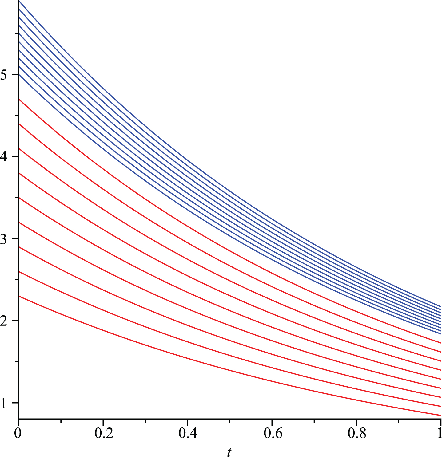
In Figure 1, red lines represent ${\underline{y}}^{P} (t; r)$ and blue lines represent ${\bar{y}}^{P} (t; r)$ .

Fig. 1

Level sets of positive part of [ii - gH]-differentiable solution defined in Example 8.1.

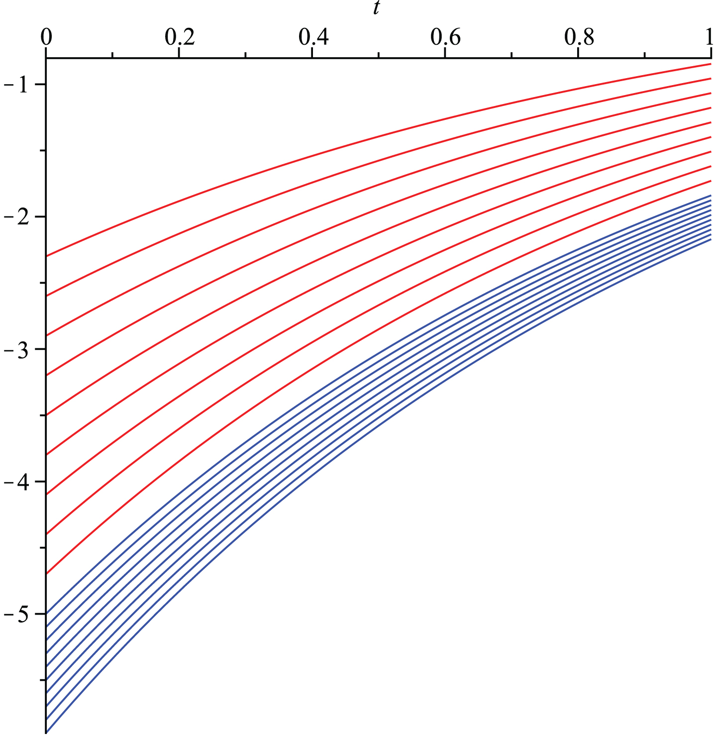
In Figure 2, red lines represent $({\underline{y}}^{P})^{'} (t; r)$ and blue lines represent $({\bar{y}}^{P})^{'} (t; r)$ .

Fig. 2

Level sets of positive part of the gH-derivative of the solution defined in Example 8.1.

In Figure 3, green lines represent ${\underline{y}}^{N} (t; s)$ and yellow lines represent ${\bar{y}}^{N} (t; s)$ .

Fig. 3

Level sets of negative part of [ii - gH]-differentiable solution defined in Example 8.1.

In Figure 4, green lines represent $({\underline{y}}^{N})^{'} (t; s)$ and yellow lines represent $({\bar{y}}^{N})^{'} (t; s)$ .

Fig. 4

Level sets of negative part of the gH-derivative of the solution defined in Example 8.1.

Example 8.2. Consider the bipolar fuzzy IVP

$\begin{matrix} {\tilde{y}}_{i . gH}^{'} (t) + \tilde{y} (t) = 2 e^{- t}, \tilde{y} (0) = ≺ [1 + 2 r, 4 - r], \\ [4 - s, 6 + s] ≻, t \in [0, 1] . \end{matrix}$ (29)

The exact (i)-solution of (29) is $\begin{matrix} y^{(r, s)} (t) = ≺ [(2 t + 1 + 2 r) e^{- t}, (2 t + 4 - r) e^{- t}], \\ [(2 t + 4 - s) e^{- t}, (2 t + 6 + s) e^{- t}] ≻, \\ r \in [0, 1], s \in [- 1, 0] . \end{matrix}$

Table 2

Global truncation errors for Example 8.2

t	Error (h=0.005)	Error (h=0.001)
0	0	0
0.1	6.5e^-04	1.31e^-04
0.2	1.2e^-03	2.29e^-04
0.3	1.5e^-03	3.00e^-04
0.4	1.7e^-03	3.48e^-04
0.5	1.9e^-03	3.79e^-04
0.6	2.1e^-03	4.28e^-04
0.7	2.3e^-03	4.69e^-04
0.8	2.5e^-03	5.03e^-04
0.9	2.7e^-03	5.30e^-04
1	2.7e^-03	5.52e^-04

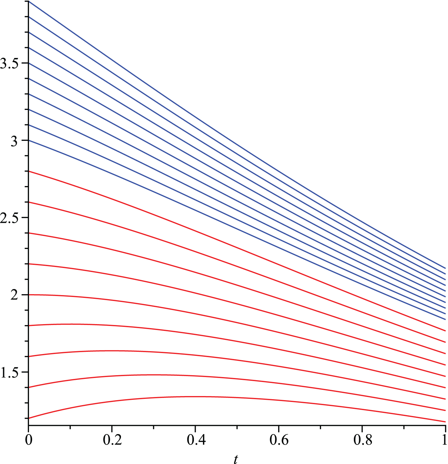
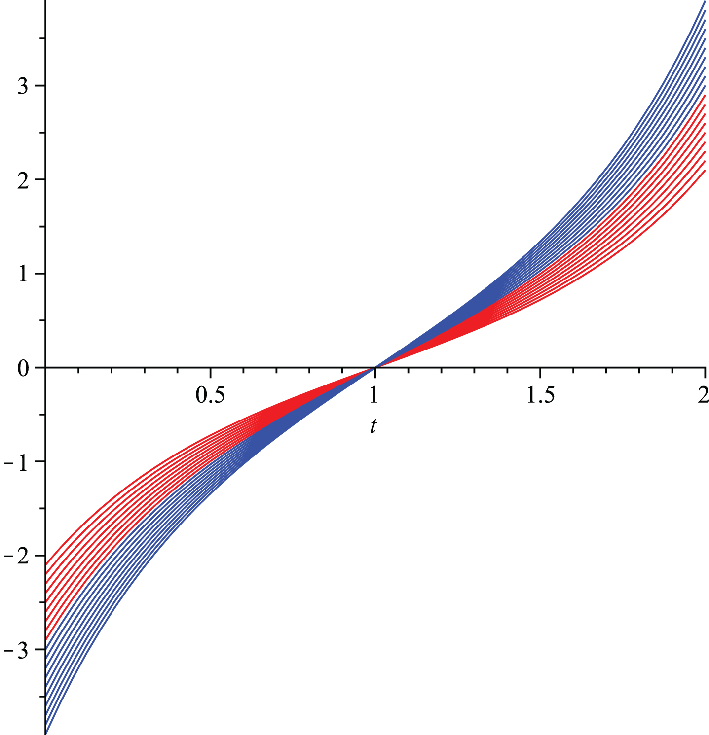
In Figure 5, red lines represent ${\underline{y}}^{P} (t; r)$ and blue lines represent ${\bar{y}}^{P} (t; r)$ .

Fig. 5

Level sets of positive part of [i - gH]-differentiable solution defined in Example 8.2.

In Figure 6, red lines represent $({\underline{y}}^{P})^{'} (t; r)$ and blue lines represent $({\bar{y}}^{P})^{'} (t; r)$ .

Fig. 6

Level sets of positive part of the gH-derivative of the solution defined in Example 8.2.

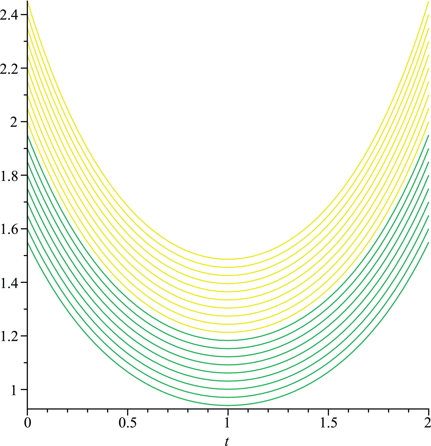
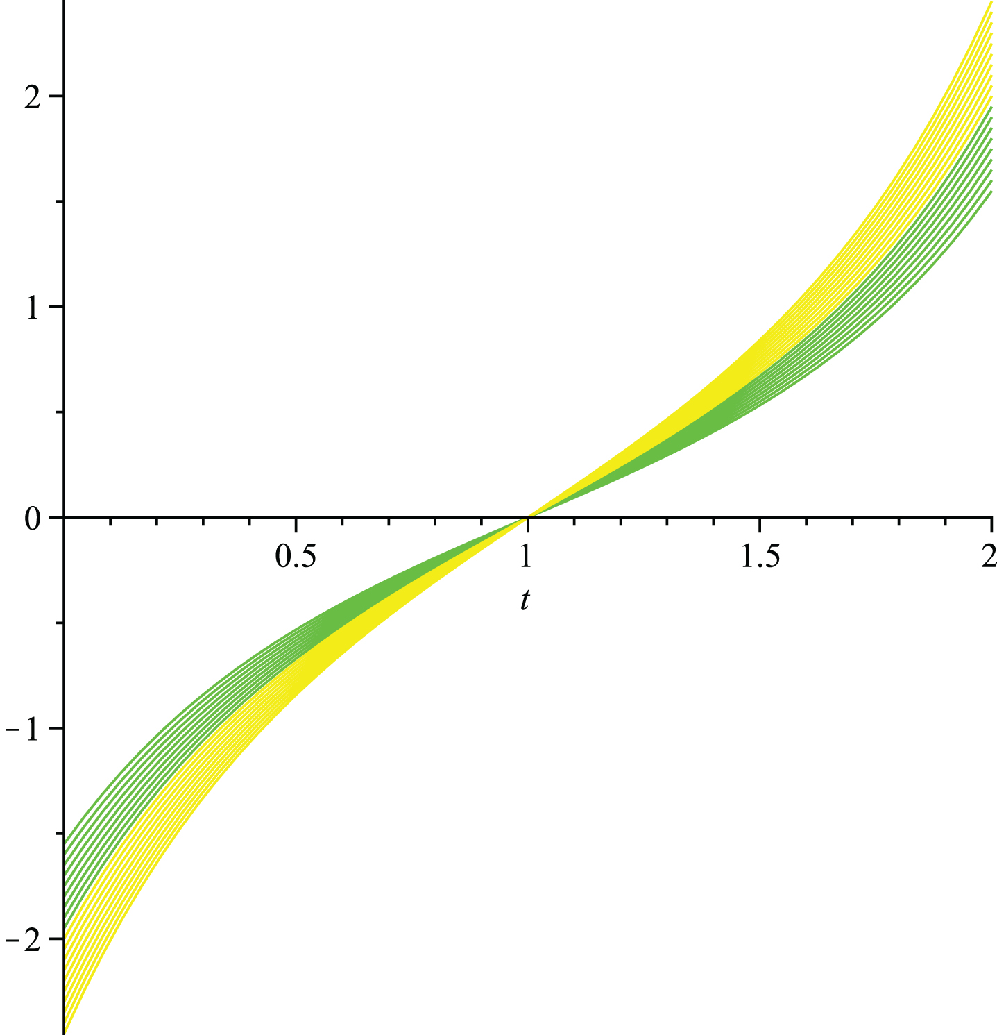
In Figure 7, green lines represent ${\underline{y}}^{N} (t; s)$ and yellow lines represent ${\bar{y}}^{N} (t; s)$ .

Fig. 7

Level sets of negative part of [i - gH]-differentiable solution defined in Example 8.2.

In Figure 8, green lines represent $({\underline{y}}^{N})^{'} (t; s)$ and yellow lines represent $({\bar{y}}^{N})^{'} (t; s)$ .

Fig. 8

Level sets of negative part of the gH-derivative of the solution defined in Example 8.2.

Example 8.3. Consider the bipolar fuzzy IVP

$\begin{matrix} {\tilde{y}}_{gH}^{'} (t) = (t - 1) \tilde{y} (t), \tilde{y} (0) = ≺ [1 + 2 r, 4 - r], \\ [1.5 - 0.5 s, 2.5 + 0.5 s] ≻, t \in [0, 2] . \end{matrix}$ (30)

Obviously the IVP is [ii - gH]-differentiable on [0,1] and at t = 1, the problem is switched to [i - gH]-differentiable. Thus t = 1 is a switching point. The solution is [ii - gH]-differentiable on [0,1] and [i - gH]-differentiable on (1,2]. The exact [ii - gH]-differentiable solution can be obtained by solving the following system $\begin{matrix} {\begin{matrix} ({\underline{y}}^{P})^{'} (t; r) = {\begin{matrix} (t - 1) ({\underline{y}}^{P}) (t; r), & t \in [0, 1], \\ (t - 1) ({\bar{y}}^{P})^{'} (t; r), & t \in (1, 2], \end{matrix} \\ ({\bar{y}}^{P})^{'} (t; r) = {\begin{matrix} (t - 1) ({\bar{y}}^{P}) (t; r), & t \in [0, 1], \\ (t - 1) ({\underline{y}}^{P})^{'} (t; r), & t \in (1, 2], \end{matrix} \\ ({\underline{y}}^{N})^{'} (t; s) = {\begin{matrix} (t - 1) ({\underline{y}}^{N}) (t; s), & t \in [0, 1], \\ (t - 1) ({\bar{y}}^{N})^{'} (t; s), & t \in (1, 2], \end{matrix} \\ ({\bar{y}}^{N})^{'} (t; s) = {\begin{matrix} (t - 1) ({\bar{y}}^{N}) (t; s), & t \in [0, 1], \\ (t - 1) ({\underline{y}}^{N})^{'} (t; s), & t \in (1, 2], \end{matrix} \\ \tilde{y} (0) = ≺ [1 + 2 r, 4 - r], [1.5 - 0.5 s, 2.5 + 0.5 s] ≻ . \end{matrix} \end{matrix}$ The exact [i - gH]-differentiable solution can be obtained by solving the following system $\begin{matrix} {\begin{matrix} ({\underline{y}}^{P})^{'} (t; r) = {\begin{matrix} (t - 1) ({\bar{y}}^{P}) (t; r), & t \in [0, 1], \\ (t - 1) ({\underline{y}}^{P})^{'} (t; r), & t \in (1, 2], \end{matrix} \\ ({\bar{y}}^{P})^{'} (t; r) = {\begin{matrix} (t - 1) ({\underline{y}}^{P}) (t; r), & t \in [0, 1], \\ (t - 1) ({\bar{y}}^{P})^{'} (t; r), & t \in (1, 2], \end{matrix} \\ ({\underline{y}}^{N})^{'} (t; s) = {\begin{matrix} (t - 1) ({\bar{y}}^{N}) (t; s), & t \in [0, 1], \\ (t - 1) ({\underline{y}}^{N})^{'} (t; s), & t \in (1, 2], \end{matrix} \\ ({\bar{y}}^{N})^{'} (t; s) = {\begin{matrix} (t - 1) ({\underline{y}}^{N}) (t; s), & t \in [0, 1], \\ (t - 1) ({\bar{y}}^{N})^{'} (t; s), & t \in (1, 2], \end{matrix} \\ \tilde{y} (0) = ≺ [1 + 2 r, 4 - r], [1.5 - 0.5 s, 2.5 + 0.5 s] ≻ . \end{matrix} \end{matrix}$ For 0 ≤ t ≤ 1, the exact [ii - gH]-differentiable solution is $\begin{matrix} y_{(2, 2)} = ≺ [(2 + r) e^{\frac{t^{2} - 2 t}{2}}, (4 - r) e^{\frac{t^{2} - 2 t}{2}}], \\ [(1.5 - 0.5 s) e^{\frac{t^{2} - 2 t}{2}}, (2.5 + 0.5 s) e^{\frac{t^{2} - 2 t}{2}}] ≻, \\ r \in [0, 1], s \in [- 1, 0] . \end{matrix}$ and for 1 < t ≤ 2, the exact [i - gH]-differentiable solution is $\begin{matrix} Y_{(1, 1)} = ≺ [(2 + r) e^{\frac{t^{2} - 2 t}{2}}, (4 - r) e^{\frac{t^{2} - 2 t}{2}}], \\ [(1.5 - 0.5 s) e^{\frac{t^{2} - 2 t}{2}}, (2.5 + 0.5 s) e^{\frac{t^{2} - 2 t}{2}}] ≻ \\ r \in [0, 1], s \in [- 1, 0] . \end{matrix}$ .

Table 3

Global truncation errors for Example 8.3

t	Error (h=0.005)	Error (h=0.001)
0	0	0
0.2	1.89e^-03	6.06e^-04
0.4	4.81e^-03	9.61e^-04
0.6	6.00e^-03	1.19e^-03
0.8	7.00e^-03	1.40e^-03
1	8.09e^-03	1.60e^-03
1.2	9.50e^-03	1.90e^-03
1.4	1.15e^-02	2.30e^-03
1.6	1.45e^-02	2.91e^-03
1.8	1.92e^-02	3.84e^-03
2	2.65e^-02	5.32e^-03

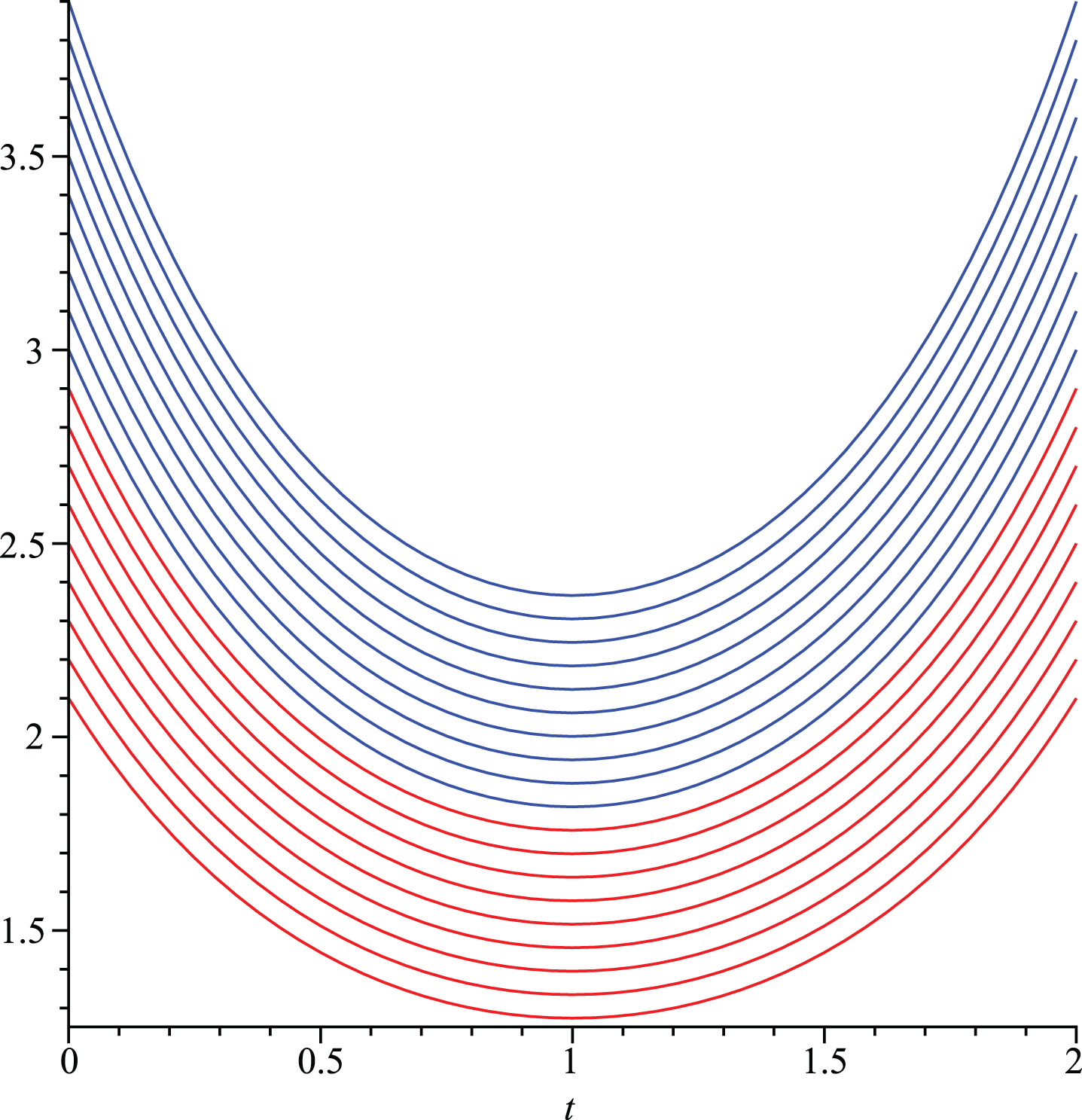
In Figure 9, red lines represent ${\underline{y}}^{P} (t; r)$ and blue lines represent ${\bar{y}}^{P} (t; r)$ .

Fig. 9

Level sets of positive part of solution defined in Example 8.3.

In Figure 10, red lines represent $({\underline{y}}^{P})^{'} (t; r)$ and blue lines represent $({\bar{y}}^{P})^{'} (t; r)$ .

Fig. 10

Level sets of positive part of the gH-derivative of the solution defined in Example 8.3.

In Figure 11, green lines represent ${\underline{y}}^{N} (t; s)$ and yellow lines represent ${\bar{y}}^{N} (t; s)$ .

Fig. 11

Level sets of negative part of solution defined in Example8.3.

In Figure 12, green lines represent $({\underline{y}}^{N})^{'} (t; s)$ and yellow lines represent $({\bar{y}}^{N})^{'} (t; s)$ .

Fig. 12

Level sets of negative part of the gH-derivative of the solution defined in Example 8.3.

9 Conclusion

Fuzzy differential equations arise in many dynamical systems. A bipolar fuzzy set is powerful tool to deal with the problems having fuzziness and vagueness. This frame is more attractive for researchers as compared to fuzzy frame. We have considered differential equations in bipolar fuzzy environment. Fuzzy initial value problem has been extended to bipolar fuzzy initial value problem where we have bipolar information about the unknown function and the initial conditions. Different types of gH-differentiability of bipolar fuzzy-valued function (FVF) are discussed. We have presented some results of gH-differentiability of bipolar FVF. Taylor expansion for bipolar FVF was obtained by considering different types of differentiability. We have demonstrated Euler method to solve bipolar fuzzy IVPs. Consistency, stability and convergence analysis of the method have been discussed. We have presented some numerical examples to show the performance and efficiency of the method. We have calculated global truncation errors. We have seen that by reducing step size, the approximate solution converges to exact solution. In future, we plan to apply predictor-corrector method to bipolar fuzzy IVPs which based on Taylor expansion. We further extend these methods to m-polar fuzzy IVPs.

Conflict of interest

The authors declare no conflict of interest.

References

Abbasbandy

and Allahviranloo

, Numerical solutions of fuzzy differential equations by Taylor method, Journal of Computational Methods in Applied Mathematics 2 (2002), 113–124.

Akram

and Arshad

, A novel trapezoidal bipolar fuzzy topsis method for group decision-making, Group Decision and Negotiation 28(3) (2019), 565–584.

Akram

, Ghulam

and Allahviranloo

, Bipolar fuzzy linear system of equations, Computational and Applied Mathematics 38(2) (2019), 69.

Aliev

R.A.

and Pedrycz

, Fundamentals of fuzzy-logic-based generalized theory of stability, IEEE Transaction on System Man and Cybernetics, Part-B Cybernetics 39 (2009), 971–988.

Allahviranloo

, Ahmady

and Ahmady

, Numerical solution of fuzzy differential equations by predictor-corrector method, Information Sciences 177 (2007), 1633–1646.

Allahviranloo

, Gouyandeh

and Armand

, A full fuzzy method for solving differential equation based on taylor expansion, Journal of Intelligent and Fuzzy Systems 29 (2015), 1039–1055.

Anastassiou

G.A.

, Numerical initial value problems in ordinary differential equations, Prentice Hall, Englewood Clifs, (1971).

Anastassiou

G.A.

, Fuzzy mathematics: Approximation theory, Studies in Fuzziness and Soft Computing 251 (2010), 267–271.

Bede

and Gal

S.G.

, Generalization of the differentiabilty of fuzzy number valued function with application to fuzzy differential equations, Fuzzy Sets and Systems 151 (2005), 581–599.

10.

Buckley

J.J.

and Feuring

, Fuzzy differential equations, Fuzzy Sets and Systems 110 (2000), 43–54.

11.

Buckley

J.J.

and Feuring

, Fuzzy initial value problem for nth-order linear differential equations, Fuzzy Sets and Systems 121 (2001), 247–255.

12.

Cano

Y.C.

and Flores

M.S.

, On new solutions of fuzzy differential equations, IEEE Transaction on System Man and Cybernetics, Part-B Cybernetics 38(1) (2008), 112–119.

13.

Chang

S.S.L.

and Zadeh

L.A.

, On fuzzy mapping and control, IEEE Transaction on Systems, Man and Cybernetics 2 (1972), 30–34.

14.

Dubois

and Prade

, Towards fuzzy differential calculus III, Fuzzy Sets and Systems 8(3) (1982), 225–233.

15.

Effati

and Pakdaman

, Artificial neural network approach for solving fuzzy differential equations, Information Science 180 (2010), 1434–1457.

16.

Epperson

J.F.

, An introduction to numerical methods and analysis, John Wiley and Sons, (2007).

17.

Esfahani

, Fard

O.S.

and Bidgoli

T.A.

, On the existence and uniqueness of solutions to fuzzy boundry value problems, Annals of Fuzzy Mathematics and Informatics 7 (2014), 15–29.

18.

Fard

O.S.

and Feuring

, Numerical solutions for linear system of first order fuzzy differential equations, Information Science 181 (2011), 4765–4779.

19.

Gasilov

N.A.

, Fatullayev

A.G.

, Amrahov

S.E.

and Khastan

, A new approach to fuzzy initial value problem, Soft Computing 18 (2014), 217–225.

20.

Ghazanfari

and Shakerami

, Numerical solution of fuzzy differential equations by extended rungekutta-like formulae of order 4, Fuzzy Sets and Systems 189 (2012), 74–91.

21.

Ghazanfari

and Shakerami

, Numerical solution of second order fuzzy differential eqaution using improved runge-kutta nystrom method, Mathematical Problems in Engineering, Article ID 803462, (2013), pp. 10.

22.

Hullermeier

, An approach to modelling and simulation of uncertain dynamical systems, Internation Journal of Uncertainity, Fuzziness and Knowledge-Based Systems 5(2) (1999), 117–137.

23.

Ivaz

, Khastan

and Neito

J.J.

, A numerical method for fuzzy differential equations and hybrid fuzzy differential equations, Abstract and Applied Analysis, Article ID 735128, 10 (2013).

24.

Jafari

, Saeidy

and Baleanu

, The variational iteration method for solving nth-order fuzzy differential equation, Information Science 10 (2012), 76–85.

25.

Jayakumar

, Kanagarajan

and Indrakumar

, Numerical solution of nth-order fuzzy differential equation by runge-kutta method of order five, International Journal of Mathematical Analysis 6 (2012), 2885–2896.

26.

Kaleva

, Fuzzy differential equations, Fuzzy Sets and Systems 24 (1987), 301–317.

27.

Khastan

and Lopez

R.R.

, On the solutions to first order linear fuzzy differential equations, Fuzzy Sets and Systems 295 (2016), 114–135.

28.

Lee

K.M.

, Bipolar-valued fuzzy sets and their basic operations, In Proceedings of the international conference, (2000).

29.

Lee

K.M.

, Comparison of interval-valued fuzzy sets, intuitionistic fuzzy sets, and bipolar-valued fuzzy sets, Journal of Fuzzy Logic Intellectual Systems 14 (2004), 125–129.

30.

Lupulescu

, Initial value problem for fuzzy differential equation under dissipative conditions, Infor-mation Sciences 178 (2008), 4523–4533.

31.

, Friedman

and Kandel

, Numerical solutions of fuzzy differential equations, Fuzzy Sets and Systems 105 (1999), 133–138.

32.

Mondal

S.P.

and Roy

T.K.

, First order linear nonhomogeneous ordinar differential equation in fuzzy environment, Math Theory Model 3 (2013), 85–95.

33.

Palligkinis

, Papageorgious

and Famelis

, Runge-kutta method for fuzzy differential equations, Applied Mathematics and Computations 209 (2009), 97–105.

34.

Parandin

, Numerical solutionof fuzzy differential equations of n-th order by runge-kutta method, Neural Computing Applications 181 (2011), 4765–4779.

35.

Pederson

and Sambandham

, The Runge-Kutta method for hybrid fuzzy differential equations, Nonlinear Analysis: Hybrid Systems 2 (2008), 626–634.

36.

Pederson

and Sambandham

, Numerical solution of hybrid fuzzy differential equation IVPs by characterization, Information Science 179 (2009), 319–328.

37.

Puri

M.L.

and Ralescu

D.A.

, Differentials of fuzzy functions, Journal of Mathematical Analysis and Application 91 (1983), 552–558.

38.

Qui

, The generalized Hukuhara differentiability of interval-valued function is not fully equivalent to the one-sided differentiability of its endpoint functions, Fuzzy Sets and Sytems, (2020).

39.

Seikkala

, On the fuzzy initial value problem, Fuzzy Sets and Systems 24 (1987), 319–330.

40.

Tapaswini

and Chakraverty

, A new approach to fuzzy initial value problem by improved Euler method, Fuzzy Information and Engineering 4(3) (2012), 293–312.

41.

Tapaswini

and Chakraverty

, Euler based new solution method for fuzzy initial value problems, International Journal of Artificial Intelligence and Soft Computing 4 (2014), 58–79.

42.

Tapaswini

, Chakraverty

and Allahviranloo

, A new approach to nth-order fuzzy differential equations, Fuzzy Sets and Systems 28(2) (2017), 278–300.

43.

Zadeh

L.A.

, Fuzzy sets, Information and Control 8 (1965), 338–353.

44.

Zhan

and Sun

, Covering-based intuitionistic fuzzy rough sets and applications in multi-attribute decision-making, Artificial Intelligence Review 53(1) (2020), 671–701.

45.

Zhan

, Sun

and Zhang

, PF-TOPSIS method based on CPFRS models: An application to unconventional emergency events, Computers and Industrial Engineering 139 (2020), 106192.

46.

Zhan

and Xu

, Two types of coverings based multi-granulation rough fuzzy sets and applications to decision-making, Artificial Intelligence Review 53(1) (2020), 167–198.

47.

Zhang

W.R.

, Bipolar fuzzy sets and relations: a computational framework for cognitive modeling and multiagent decision analysis, In Proceedings of IEEE Conference (1994), 305–309.

48.

Zhang

W.R.

, Bipolar fuzzy sets, IEEE International Conference on Fuzzy Systems Proceedings 1 (1998), 835–840.