Optimal order strategy for channels under different supply risk levels

Abstract

We consider an order problem for two channels consisting of one common retailer and two competing suppliers that are subject to supply uncertainty. A new concept of supply risk level (SRL) of a channel is proposed to quantitatively characterize the supply risk of the channel due to supply uncertainty. Under different SRLs, we study the order strategies for the two channels in integrated and decentralized supply chains. Regardless of whether the game is integrated or decentralized, we find that the different SRLs give rise to a difference between the belief-degree costs of the two channels that directly influences the optimal order strategy, market supply and profit of each channel. This implies that the decision maker of the supply chain can take different risk attitudes toward the supply uncertainty of the two channels to adjust the potential market supply and profit of each channel because the decision maker generally replaces the SRL with his or her risk preference. Under given SRLs, we find that integration is a better strategy than decentralization. However, the channel profit with a higher belief-degree cost under decentralization is greater than that under integration in some cases. Finally, proper risk preferences for both channels are suggested to strike a balance between supply reliability and supply risk.

Keywords

Supply uncertainty supply risk level supply chain competition belief-degree cost

1 Introduction

Supply uncertainty is common in supply chain competition and has various causes, for example, vegetable yields are affected by, among other factors, weather conditions, diseases and insects. Many factors, such as transportation time, weather conditions and traffic conditions, directly influence the quantities of fresh fruits supplied in the market. Media reports reveal that the supply rate for TSMC, who is a non-competitive supplier of Apple and provides the fingerprint sensor for Apple, is only around 70%-80% [5, 27]. The mismatch of supply and demand due to supply uncertainty can cause losses to both upstream and downstream firms in supply chains. Firms may use multi-source procurement strategies to alleviate the risk caused by supply uncertainty [35]. In multi-source procurement problems, uncertain supply is usually assumed to be a random variable (such as [1, 31]).

However, in some supply chain competition problems, there may be no observed data about uncertainties in supply that cannot be exactly predicted in advance, such as the supply uncertainty caused by a sudden accident. Thus, people are only able to make subjective judgements about such events, and as a result, probability theory is no longer applicable.

Therefore, this paper studies how to characterize uncertain information about supply in a competitive supply chain environment by using uncertainty theory [20] instead of probability theory in the present of no or little observed data, which is an essential tool to cope with experts’ subjective judgements about uncertain information and depict uncertain information about supply in the context of supply chain risk management. Supply uncertainty occurs when the quantity supplied to a downstream firm, such as a retailer, is not the quantity that the firm ordered. For example, consider a supplier who sells perishable or fragile products (such as fresh fruits or glass items) to a retailer. Because of transportation time, weather conditions, traffic conditions, or other factors, the quantity of products received by the retailer does not equal the order quantity. In fact, the retailer receives a certain percentage of the order quantity with a certain belief degree. The certain belief degree can only be subjectively evaluated because of the absence of additional information. Obviously, the belief degree of how high the ratio of the order quantity can reach is important to the retailer because its magnitude directly affects the retailer’s order strategy and profit. This belief degree usually takes a moderate value (50%) in theoretical research. However, this approach is often inappropriate due to possibility of large deviations from the actual value when there are insufficient data about uncertain supply information. This implies that decision makers need to make a tradeoff between supply reliability and supply risk in the absence of adequate data. Based on this motivation, a concept of supply risk level (SRL) of a channel is proposed to quantitatively depict the risk caused by supply uncertainty. Under different SRLs, we research the order strategy for the two channels in integrated and decentralized supply chains and construct corresponding models. Specifically, we attempt to answer the following questions: How can one apply the SRLs to quantitatively characterize the supply risks of channels due to supply uncertainty? In integrated and decentralized supply chains, what is the key factor affecting the channel competition, and how do the SRLs affect the key factor and thus affect the order strategy and profits of channels? For given SRLs, is integration a better strategy than decentralization? Based on the impact of SRLs on order strategy, can proper risk preferences be selected to strike a balance between supply reliability and supply risk in a supply chain with supply uncertainty?

To answer these questions, we investigate an order problem for two channels composed of one common retailer and two competing suppliers that are subject to supply uncertainty. SRLs are used to quantitatively characterize the uncertain supply quantities of the two channels in the integrated and decentralized supply chains. Under different SRLs, we construct the corresponding models and find the key factor affecting supply chain competition. We further analyze the impact of the key factor and SRLs on the order quantities and profits of the channels in the decentralized (or integrated) game. By comparing the two equilibria in the two games, we examine the value of integration under different SRLs. Moreover, by striking a balance between supply reliability and risk, we suggest a proper risk preference selection strategy for the decision maker of each channel.

Compared with the existing literature, our paper has two main contributions. On the one hand, we quantitatively characterize the supply risk level of a channel due to supply uncertainty and introduce the attitudes of decision makers toward uncertain supply risk into optimal order questions under dual supply uncertainties, which is never done to the best of our knowledge. On the other hand, we continue to contribute to the field of supply chain risk management by considering both multi-dimensional uncertain information and all different risk attitudes of decision makers. Many scholars [8 , 38] only research the risk management problem of one-dimensional uncertain information and consider only a single situation of different decision makers’ risk attitudes (one is risk-averse and the other is risk-neutral). Nevertheless, the case of two-dimensional uncertain information and all different risk attitudes of decision makers are simultaneously studied in this paper. Moreover, a suggestion to the decision makers who have no special preference for supply risk is given and shows that the expectation supply is not always appropriate. We have performed similar works in Liu et al. [23] and Liu et al. [24]. The difference between this paper and the above two papers lies in the different problems studied and the different types of risks depicted. Liu et al. [23] consider the profit risk levels of a supply chain under uncertain basic market demand and uncertain product review in the two-period dynamic pricing problems. Liu et al. [24] study a retailer’s decision selection problem (the retailer enforces demand management by adjusting prices, seeks the backup supplier to make up for the lack of products or mixes the two decisions) while characterizing the reliability of uncertain supply in satisfying demand (the risk attitude of decision makers toward uncertain supply in satisfying demand). However, in this paper, we characterize the supply risk level of a channel due to supply uncertainty related to the optimal order problem.

Different from the existing literature, the main specific conclusions are as follows. First, we use uncertainty theory to quantitatively characterize the SRL of a channel, and from this, the concept of belief-degree cost of a channel (or supplier) is proposed. A channel’s belief-degree cost comprehensively reflects the supply uncertainty and the risk attitude of the decision maker. It embodies the decision maker’s ability to comprehensively address information uncertainty and control the resulting risk. The belief-degree cost of a channel decreases with its SRL; that is, it depends on the central planner’s (or retailer’s) attitude toward supply risk in the integrated (or decentralized) game.

Second, our results demonstrate that in either the integrated or decentralized game, the different risk attitudes of the decision maker (i.e., the central planner in the integrated game or the retailer in the decentralized game) toward supply uncertainty give rise to differences in the belief-degree costs of the two channels. When the difference in belief-degree costs is significant, the market is monopolized by the channel with a sufficiently low belief-degree cost. Otherwise, when the difference in belief-degree costs is not significant, the decision maker is willing to provide a larger market supply from the channel with a lower belief-degree cost and obtain higher profits. Furthermore, if the decision maker has a risk-loving attitude toward the supply risk of this channel or a risk-averse attitude toward that of the other channel, then the profit of the former channel increases because the market supply from this channel increases. This conclusion is intuitive because an adventurous decision maker may obtain higher profits by providing greater market supply. If the decision maker is averse to supply risk in the competing channel, the decision maker will decrease the market supply from the competing channel and then increase the market supply from the first channel. This also implies that the decision maker of the supply chain can take different risk attitudes toward the supply uncertainty of the two channels to adjust the potential market supply and profits of each channel.

Third, under different SRLs, our results show that integration is a better strategy than decentralization because the total market supply and profits of the supply chain are higher in the integrated game than in the decentralized game. However, in some cases, the profit of the channel with a higher belief-degree cost is higher under decentralization than under integration. This is because in a decentralized supply chain, a decrease or an increase in the supply chain’s total profit is primarily due to a decrease or an increase in the profits of the channel with the lower belief-degree cost, in contrast to the case of an integrated supply chain. Therefore, when the risk attitudes of the decision maker toward the supply uncertainty of the two channels increase the difference in belief-degree cost between the two channels, the profit of the channel with a higher belief-degree cost is lower than that of this channel’s rival, regardless of whether one considers the integrated or decentralized game. Nevertheless, in the integrated game, the low extent is greater than that in the decentralized game, and as a result, the profit of the channel with a higher belief-degree cost is lower in the integrated game than in the decentralized game in this case.

Finally, we propose a proper risk preference for the decision maker of each channel that attempts to maximize the order quantities. Under the suggested risk preference, our results show that the expected supply is not always appropriate in either the decentralized or integrated game, and the decision maker’s attitude toward the supply uncertainty of each channel in the decentralized game should be more conservative than that in the integrated game due to double marginal utility.

The rest of the paper is organized as follows. In Section 2, we review the literature relevant to our study. In Section 3, we describe and build the models in the integrated and decentralized supply chains. In Section 4, we compare the equilibria in the integrated and decentralized games. In Section 5, we suggest a proper risk preferences for the decision makers of two channels. Finally, the conclusions are summarized in Section 6.

2 Literature review

Contributions to four streams of the literature are relevant to this study: supply uncertainty, supply chain competition, supply chain risk measures, and uncertainty theory and its application.

The existing literature on supply uncertainty can be divided into three lines of research: the first focusing on random yields [10 , 32], the second focusing on lead times (see a comprehensive review in Zipkin [42]), and the third focusing on supply disruptions (for reviews, see Tang [33]). In the first two lines, scholars often assume that the supply level is a random function of the input level and that the lead time is also a random variable. In the third line, supply disruptions, which are usually infrequent and temporary, result in significant shocks to the system. Hendricks et al. [16] offer numerous examples demonstrating that failing to recognize the possibility of supply disruptions can have devastating economic consequences. Yu et al. [39] comprehensively describe how the concept of disruption management is applied and what impact it has. Heckmann et al. [15] regard supply disruption as a type of network risk based on a summary of relevant supply chain risk categories. Li et al. [18] investigate how the manufacturer, in a better financial situation, may use ex ante penalty terms and ex post financial assistance to force the supplier to recover its production capability to the greatest extent possible. However, the above studies do not describe the supply uncertainty levels, whereas our study uses SRLs of channels to quantitatively characterize uncertain supply risk levels and analyzes their impact on order quantities and profits.

Our study is related to the literature on supply chain competition with uncertain information. Supply chain competition include two forms: within-chain competition [14] and chain-to-chain competition [2, 37]. The uncertain information causing the mismatch between supply and demand usually includes supply uncertainty or/and demand uncertainty [28, 34]. Some papers deal with uncertain information and within-chain competition simultaneously in contract design problems. For example, Lee et al. [17] employ a screening model to examine the supply chain contracting problem for two suppliers competing to sell their partial substitute products to one common retailer. They use a linear demand function to denote the market clearing price and assume that the market size is a random variable representing the demand uncertainty. Their main results show that suppliers prefer the two-part tariff contract to the quantity discount contract. Li et al. [19] consider a contract design problem for two competing suppliers working with a common retailer whose type is either low-volume or high-volume. The flexible supplier has a high variable cost, while the efficient supplier has a low variable cost and a fixed cost. A menu of contracts is offered by each supplier to the common retailer. They analyze how the efficient supplier’s fixed cost influences the optimal contract design and the competition between the two suppliers. However, the two papers mentioned above do not consider the supply chain risk caused by uncertain information.

The third stream of relevant literature focuses on the supply chain risk measures. There are many quantization methods applied for supply chain risk, such as variance, standard deviation, mean-variance, value-at-risk, conditional-value-at-risk. These quantitative measures aim at describing the interaction of uncertainty and the extent of its related harm or benefit. We briefly introduce several supply chain risk measures. Variance or standard deviation are widely applied in measuring the supply chain risk, although some scholars consider that they are problematic as risk measures in general [4, 9]. Both the two methods are to evaluate the wideness of a distribution and think about the positive and negative deviations (i.e, upside and downside risk) from expected revenues [30]. Therefore, the absolute value of a deviation is considered as risky as a equal-sized loss. However, Cox [9] demonstrates that in the theoretical decision analysis and financial economics, the standard deviation analysis is restricted, whereas the mean-variance analysis is applicable. Chen et al. [7] use the mean-variance analysis to revisit some basic inventory models and study how to efficiently carry out a systematic mean-variance tradeoff analysis. Buzacott et al. [6] use mean-variance analysis to study a commitment option contract. Comparing with the related work of expected utility theory, they show that many results remain valid and a downside risk measure may be more appealing to companies. Value-at-risk and conditional-value-at-risk are applied in portfolio problems as percentile measures of downside risks. The two methods characterize different parts of a profit or loss distribution and their use is determined by the goal of the decision maker as well as by the availability and quality of distribution estimates [30]. Value-at-risk is defined as a threshold value relevant to a specified confidence level of outcomes and does not account for the distribution properties beyond the confidence interval. However, conditional-value-at-risk could cover drawbacks of previous risk measures such as value-at-risk. In fact, it could add positive points to previous risk measures. For instance, it provides an indication about the severity of loss and is a coherent and convex risk measure [3]. It has become a popular well-behaved risk measure due to its mathematical properties that are especially suitable for optimization problems [29, 30]. Heckmann et al. [15] comprehensively review the existing approaches to quantify supply chain risks by setting the focus on the supply chain risk definition and relevant concepts. Value-at-risk and conditional-value-at-risk are defined based on the assumption that the distribution function of a random variable is not less than a given confidence level. The above methods are based on probability theory. However, as stated in the Introduction, probability theory does not apply to problems with uncertain information having no or little observed data. In addition, it is difficult or even impossible to obtain the analytical solutions of the problems with multi-dimensional uncertain information, and thus it is difficult to draw general management implications for such issues. Therefore, we use uncertainty theory to study the optimal order problem with dual supply uncertainties and solve the analytical solutions. Moreover, through analytical analyses, the management significance of the problem is finally obtained.

Finally, our study is relevant to literature on the uncertainty theory and its applications. Uncertainty theory is founded by Liu [20] and refined by Liu [22]. Uncertainty theory is now regarded as a branch of axiomatic mathematics for handling human language and modeling human uncertainty, and is widely applied in supply chain management. For example, it is applied in dynamic recruitment problems [40] and principal-agent problems [36, 41]. We have been engaged in supply chain risk management research using uncertainty theory. For instance, we consider a contract problem by using uncertainty theory to characterize the uncertain variable costs of the two suppliers and the uncertain external demand, and analyze the impact of the confidence levels on the selection of the retailer with two types [25]. We research two-period dynamic pricing problems under considering the profit risk levels of a supply chain with uncertain basic market demand and uncertain product review [23]. We study a retailer’s decision selection problem (the retailer enforces demand management by adjusting prices, seeks a backup supplier to make up for the lack of products or mixes the two decisions) while characterizing the reliability of uncertain supply in satisfying demand (the risk attitude of decision makers toward uncertain supply in satisfying demand) [24]. Different from the above three works [23 –25], this paper considers an order problem for the channels with dual supply uncertainties. Furthermore, we analyze the impact of different SRLs on the order quantities of channels and suggest proper risk preferences for the decision makers of channels to balance supply reliability and supply risk.

3 The model

3.1 Problem description

We consider a supply chain with two suppliers, indexed by i, j ∈ {1, 2} (i ≠ j), and one common retailer (she). The suppliers sell the congeneric products to the retailer and compete on the quantity. For convenience, the supply chain composed of supplier i (he) and the retailer is called as channel i. The main notation is described in Table 1.

Table 1
List of main notation

Notation Description

ξ _i Uncertain supply ratio of channel i

Φ _i Uncertain distribution of ξ_i

$Φ_{i}^{- 1}$ Inverse uncertain distribution of ξ_i

θ _i Supply risk level (SRL) of channel i

Q _mi Channel i’s θ_i-supply-quantity

c _1i Production cost per unit of supplier i

c _2i Successful delivery cost per unit of supplier i

c _i Belief-degree cost of channel i

p _i Market clearing price of channel i

A Market size

γ competitive intensity

C_i = A - c_i Difference of market size and belief-degree cost of channel i

β = C₁/C₂ Difference in belief-degree costs between the two channels

S Profit of the total supply chain

s _i Profit of channel i

v Profit of the retailer

u _i Profit of supplier i

Decision variables

q _i Order quantity of channel i

w _i wholesale price of supplier i

W_i = w_i - c_i Marginal profit of supplier i

Notation	Description
ξ _i	Uncertain supply ratio of channel i
Φ _i	Uncertain distribution of ξ_i
$Φ_{i}^{- 1}$	Inverse uncertain distribution of ξ_i
θ _i	Supply risk level (SRL) of channel i
Q _mi	Channel i’s θ_i-supply-quantity
c _1i	Production cost per unit of supplier i
c _2i	Successful delivery cost per unit of supplier i
c _i	Belief-degree cost of channel i
p _i	Market clearing price of channel i
A	Market size
γ	competitive intensity
C_i = A - c_i	Difference of market size and belief-degree cost of channel i
β = C₁/C₂	Difference in belief-degree costs between the two channels
S	Profit of the total supply chain
s _i	Profit of channel i
v	Profit of the retailer
u _i	Profit of supplier i
Decision variables
q _i	Order quantity of channel i
w _i	wholesale price of supplier i
W_i = w_i - c_i	Marginal profit of supplier i

The suppliers and the retailer are affected by supply uncertainty. The uncertainty may be caused by transportation disruption, natural disasters, labor strikes, and so on, which are considered to be outside the control of the suppliers and the retailer. We assume that the retailer orders q_i units of products from supplier i and that supplier i manufactures all the products; however, the retailer receives ξ_iq_i due to supply uncertainty. We assume ξ_i (called an uncertain supply ratio) is an uncertain variable on the interval [0, 1] with uncertainty distribution Φ_i. In the extreme cases, the products are completely damaged and broken and can not be used, so the retailer does not receive any product when ξ_i = 0; when ξ_i = 1, all products are in good condition and the retailer receives q_i units of the products. This assumption is similar to Adhikari et al. [1] and Wu et al. [35], and the difference is that the supply ratio is assumed to be random in the above two studies. As mentioned in the Introduction, it is not appropriate to make random assumptions in the absence of data. The uncertain variables ξ₁ and ξ₂ are assumed to be independent, and all the participants know their distributions that are estimated by the experts familiar with the underlying mechanisms of supply uncertainties. Simultaneously, the suppliers and retailer have no more information about supply uncertainty but only know the distributions of uncertain supply ratios.

We use the confidence level α_i to measure the supply uncertainty level or the supply risk level of supplier i: the lower α_i is, the greater the uncertainty or the higher the supply risk level. For convenience of understanding, let θ_i = 1 - α_i be the supply risk level of supplier i, which is also the supply risk level of channel i (SRL of channel i, for short), and thus a higher value of θ_i means a higher supply risk level. The SRL θ_i is the degree of belief in an unsuccessful result and reflects channel i’s supply risk level. Under the SRL θ_i, the supply quantity of supplier i can be expressed as Q_0i belonging to ${Q_{0 i} | M {ξ_{i} q_{i} ⩾ Q_{0 i}} ⩾ 1 - θ_{i}},$ which is a set of supplier i’s supply quantities. Obviously, supplier i’s supply quantity Q_0i depends not only on the retailer’s order quantity but also on the SRL of channel i. Given the order quantity q_i, supplier i’s θ_i-supply-quantity Q_mi (q_i, θ_i) can be denoted by

$\begin{matrix} Q_{mi} (q_{i}; θ_{i}) = max {Q_{0 i} | M \\ {ξ_{i} q_{i} ⩾ Q_{0 i}} ⩾ 1 - θ_{i}} . \end{matrix}$ (1)

This implies that if the retailer orders q_i units of products, supplier i supplies Q_mi (q_i ; θ_i) units of products with the degree of belief in a successful result of not less than 1 - θ_i (i.e., with a SRL θ_i). This method is similar to that of Liu et al. [23] and Liu et al. [25]. The difference is that the above two papers consider information uncertainty from the perspective of a supply chain’s profit, while this paper addresses supply uncertainty from the perspective of the quantity supply. Moreover, the method we consider is reasonable and consistent with reality. For example, consider a supplier that sells perishable or fragile products, such as fresh fruits or glass items, to a retailer. Due to transportation time, weather conditions, traffic conditions, or other factors, the quantity of products received by the retailer is a certain percentage of the order quantity with a certain belief degree. This belief degree can only be subjectively assessed because no further information is available. Obviously, the belief degree on how high the ratio of the order quantity can reach is important to the retailer because its magnitude directly affects the retailer’s order strategy and profit.

In Sections 3 and 4, we assume that the SRLs are determined by the experts’s experience, which means that they are exogenous and known to all the participants. For example, the experts estimate the SRL of fresh fruits based on their experience of the rate of decay of fruit, temperature on the day of delivery and delivery distance. In reality, a channel’s decision maker, such as a retailer or supplier, can be considered an expert because he or she has a think tank to assess supply risks or has enough experience on supply risk. In the absence of sufficient information to obtain the exact SRL of a channel, the decision maker generally determines her order quantity according to her risk preference instead of SRL. That is, the decision maker’s attitude toward supply risk directly affects her order strategy and profit. Therefore, in Section 5, a proper selection of SRLs is suggested to balance the supply reliability and risk, which means that the neutral attitude toward risk might not be the optimal choice for a rational retailer.

Based on this view, when the SRL θ_i is one, supplier i or the retailer believes that the supply quantity Q_mi (q_i ; 1) is the order quantity q_i (i.e., Q_mi (q_i ; 1) = q_i), whereas he or she knows only that the belief degree of this result is not less than zero because there is no further information available. In real life, only an extremely risk-loving retailer might select this risk level because she believes that the supply quantity is her order quantity under the highest supply risk. When the SRL is one half, the supply quantity is the expected supply (i.e., Q_mi (q_i ; 0.5) = E [ξ_iq_i]). When the SRL is zero, the supply quantity is zero (i.e., Q_mi (q_i ; 0) =0). No retailer will select this risk attitude in real life because the supply quantity with a belief degree of one hundred percent is zero due to supply uncertainty. In general, a risk-loving retailer may select a SRL of more than one half, while a risk-averse retailer may select a SRL of less than one half. A rational retailer may select the SRL of one half; that is, the retailer is risk neutral.

Lemma 1. Channel i’s θ_i-supply-quantity $Q_{mi} (q_{i}; θ_{i}) = Φ_{i}^{- 1} (θ_{i}) q_{i}$ , where $Φ_{i}^{- 1} (θ_{i})$ is called as channel i’s supply ratio under the SRL θ_i (channel i’s supply ratio, for short).

Supplier i faces two marginal costs: c_1i per unit of production and c_2i per unit of successful delivery under a given SRL θ_i. If supplier i produces q_i units of the products and the retailer receives ξ_iq_i units, supplier i’s total cost is c_1iq_i + c_2iQ_mi (q_i ; θ_i) under the SRL θ_i. To simplify notation, we define $c_{i} = c_{1 i} / Φ_{i}^{- 1} (θ_{i}) + c_{2 i}$ , which essentially represents the total unit cost of products under the SRL θ_i, and thus the total cost becomes c_iQ_mi (q_i ; θ_i). We call c_i suppler i’s belief-degree cost under the SRL θ_i (supplier i’s belief-degree cost, for short). Because supplier i’s cost is also that of channel i, c_i is also called channel i’s belief-degree cost. The belief-degree cost c_i is decreasing in the SRL θ_i; that is, the lower the SRL, the higher the belief-degree cost. In the converse case, the belief-degree cost of suppler i is lower. In essence, a decrease in the supply risk level comes at the cost of a considerable increase in the total unit cost of production. In other words, a risk-averse decision maker believes that the belief-degree cost of the channel is higher, while a risk-loving one believes that the belief-degree cost is lower. To understand this concept intuitively, let us take a numerical example. Assume that c₁₁ = 2, c₂₁ = 1 and $ξ_{1} \sim L (0, 1)$ , meaning that the experts estimate the uncertain supply ratio is on the interval [0, 1]. Then, the total unit cost of products of channel 1 is estimated as c₁ = 2/[0 * (1 - θ₁) +1 * θ₁] +1 = 2/θ₁ + 1 under the SRL θ₁. This implies that the decision maker of channel 1 regarded 11 as the total unit cost of channel 1 if its decision maker is risk-averse and has a lower risk level θ₁ = 0.2. The belief-degree cost of channel 1 is estimated as 3.5 if its decision maker is a risk lover and has a higher risk level θ₁ = 0.8. In the extreme case, the completely risk-averse decision maker (θ₁ = 0) believes that the belief-degree cost is infinite; then, the supplier is unwilling to supply the products, and the retailer is also unwilling to purchase the products. Oppositely, the completely risk-loving decision maker (θ₁ = 1) believes that the belief-degree cost is 3, which is equal to the actual total unit cost c₁₁ + c₂₁ with no product loss. The belief-degree cost is estimated to be no less than c₁₁ + c₂₁ or even infinite for risk-averse or risk-loving decision makers because they believe that some or even all products may not be delivered successfully due to supply uncertainty.

In a supply chain, for given costs of production and successful delivery (c_1i and c_2i are constant), a supplier’s belief-degree cost comprehensively reflects the supply uncertainty and the risk attitude of decision makers because the inverse uncertain distribution $Φ_{i}^{- 1}$ describes the supply uncertainty and θ_i represents the risk attitude of decision makers. If the decision makers can assess the distribution of uncertain supply more accurately (for example, the estimation of distribution is tightened to be in the interval [0.6, 0.8] ⊂ [0, 1]), then the supply uncertainty is eased. Furthermore, the risk attitude of decision makers is properly selected (for example, it is closer to the actual level of supply uncertainty); as a result, the decision makers can more accurately estimate the total unit cost (belief-degree cost). Therefore, the belief-degree cost embodies the decision maker’s ability to comprehensively address information uncertainty and control the risk caused by information uncertainty. This definition is similar to that of Liu et al. [26]. Liu et al. [26] assume that the production costs of two supply chains and the price noise are uncertain, while the supply ratios of two channels are uncertain in this paper. What they have in common is that the information uncertainty is ultimately reflected in the belief-degree cost.

It is noted that even if the SRLs of the two channels are the same, the size relationship of their belief-degree costs could change with the same SRL, and more so with different SRLs (see Fig. 1). From Fig. 1, it is clear that on the left-hand side of θ₀, the belief-degree cost of channel 1 is lower than that of channel 2 whether the SRLs of the two channels are the same or different (i.e., c₁ < c₂ if θ < θ₀), whereas the opposite conclusion is reached for the right-hand side of θ₀ (i.e., c₁ > c₂ if θ > θ₀). Therefore, under different SRLs, the belief-degree costs of the two channels are heterogenous, and their size relationship could be changed. The reason for this is that the costs of production and successful delivery may not be the same for the two channels, even though the distributions of uncertain supply rate of the two channels and the risk attitudes of the decision makers are the same.

Fig. 1

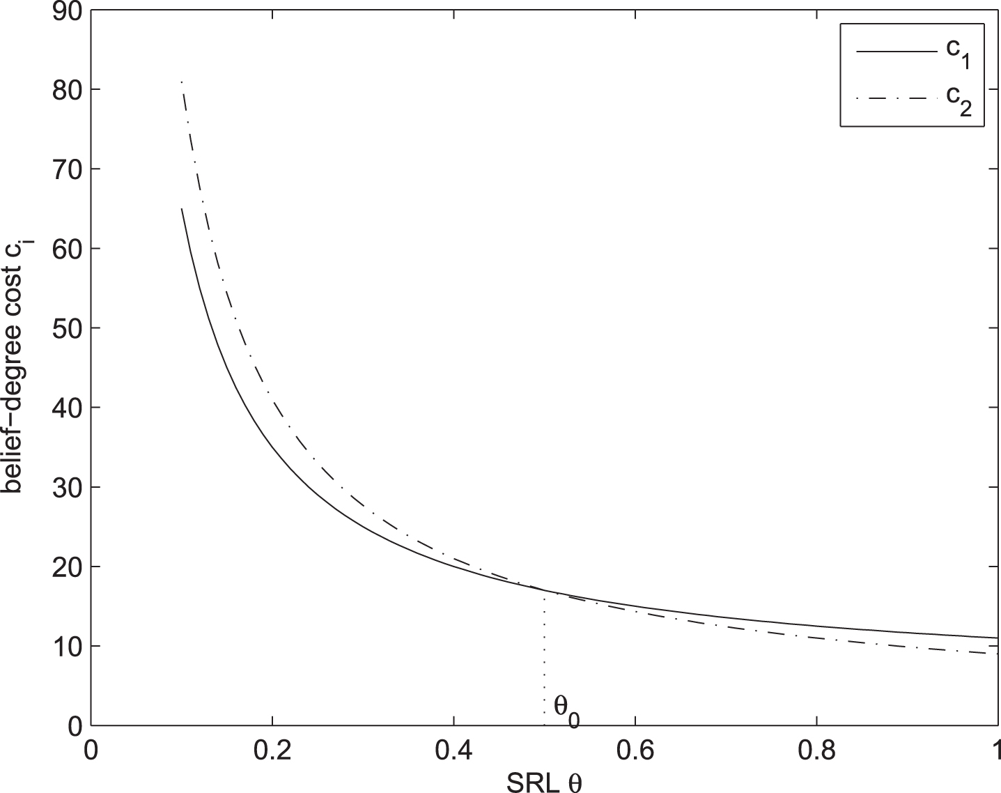
Effect of SRL θ on belief-degree cost c_i.

Under the SRL θ_i, the suppliers compete in a market with a linear demand function. And the market clearing price can be denoted by $p_{i} (q_{1}, q_{2}; θ_{1}, θ_{2}) = A - Q_{mi} (q_{i}; θ_{i}) - γ Q_{mj} (q_{j}; θ_{j}),$ where p_i (q₁, q₂ ; θ₁, θ₂) is the market clearing price, A represents the market size and γ ∈ [0, 1] measures the competitive intensity. To exclude the non-interesting case where neither party sells to the market, we assume A > c_i > 0.

The sequence of events is presented as follows.

The retailer orders q_i units of the products from supplier i.

Supplier i supplies Q_mi (q_i ; θ_i) units of the products to the retailer under the SRL θ_i.

Under the SRL θ_i, the market is cleared from the total supply chain and cash flows are distributed to each part.

3.2 Integrated supply chain

We first study the situation in which the supply chain is integrated, i.e., the two suppliers and the retailer are fully integrated to achieve the maximum profit of the entire supply chain. We use a central planner to represent the two suppliers and the retailer. In this subsection and the following, we only provide the models, the results and the corresponding properties under the given SRLs of both channels, and we will discuss the retailer’s risk choice in Section 5. Note that the SRLs θ₁ and θ₂ of the two channels may be the same or different. The former case means that the entire supply chain bears a common risk, whereas the latter case implies that the two channels bear different risks, reflecting the central planner’s different attitudes toward the supply risks of the two channels.

The goal is to maximize the profit of the supply chain under the SRL θ_i, which can be expressed as

$\begin{matrix} max_{q_{1}, q_{2} ⩾ 0} S (q_{1}, q_{2}; θ_{1}, θ_{2}) = \\ max_{q_{1}, q_{2} ⩾ 0} \sum_{i = 1}^{2} (p_{i} (q_{1}, q_{2}; θ_{1}, θ_{2}) - c_{i}) Q_{mi} (q_{i}; θ_{i}) . \end{matrix}$ (2)

The following theorem characterizes the optimal solution and the corresponding profits for the integrated supply chain. For convenience, let C_i = A - c_i, which is increasing in θ_i, and β = C₁/C₂. The parameter β means the difference in belief-degree costs between the two channels, which is increasing in θ₁, and is decreasing in θ₂. The parameter β > 1 implies that the belief-degree cost of channel 1 is lower than that of channel 2.

Theorem 1. The optimal solution of the integrated supply chain has the following characteristics.

If β ⩽ γ, the supply chain’s optimal order quantities ${\bar{q}}_{1} = 0$ and ${\bar{q}}_{2} = C_{2} / (2 Φ_{2}^{- 1} (θ_{2}))$ . Moreover, channels 1, 2 and the total supply chain’s profits ${\bar{s}}_{1} = 0, {\bar{s}}_{2} = C_{2}^{2} / 4$ and ${\bar{s}}_{1} + {\bar{s}}_{2} = C_{2}^{2} / 4$ .

If γ < β < 1/γ, chain i’s optimal order quantity ${\bar{q}}_{i} = (C_{i} - γ C_{j}) / [(2 - 2 γ^{2}) Φ_{i}^{- 1} (θ_{i})]$ . Moreover, channel i and the total supply chain’s profits ${\bar{s}}_{i} = C_{i} (C_{i} - γ C_{j}) / (4 - 4 γ^{2})$ and ${\bar{s}}_{1} + {\bar{s}}_{2} = (C_{1}^{2} - 2 γ C_{1} C_{2} + C_{2}^{2}) / (4 - 4 γ^{2})$ . Particularly, when β = 1, we have ${\bar{q}}_{i} = C_{1} / [(2 + 2 γ) Φ_{i}^{- 1} (θ_{i})]$ , ${\bar{s}}_{i} = C_{1}^{2} / (4 + 4 γ)$ and ${\bar{s}}_{1} + {\bar{s}}_{2} = C_{1}^{2} / (2 + 2 γ)$ .

If β ⩾ 1/γ, the supply chain’s optimal order quantities ${\bar{q}}_{1} = C_{1} / (2 Φ_{1}^{- 1} (θ_{1}))$ and ${\bar{q}}_{2} = 0$ . Moreover, channels 1, 2 and the total supply chain’s profits ${\bar{s}}_{1} = C_{1}^{2} / 4, {\bar{s}}_{2} = 0$ and ${\bar{s}}_{1} + {\bar{s}}_{2} = C_{1}^{2} / 4$ .

Theorem 1 implies that in the integrated supply chain, whether the market is monopolized by one channel depends on the two channels’ belief-degree costs which reflect the supply uncertainty and the risk attitude of the central planner. Under given SRLs θ₁ and θ₂, when the difference in belief-degree costs between the two suppliers is significant (or the competitive intensity is higher), the central planner places an order only from the channel with a lower belief-degree cost (i.e., situation (i) or (iii)). Otherwise (i.e., situation (ii)), the central planner orders the products from the two channels. In fact, β ⩽ γ and γ ∈ [0, 1] mean that supplier 2’s belief-degree cost is far lower than that of supplier 1, whereas β ⩾ 1/γ indicates that his belief-degree cost is far higher than that of supplier 1. Thus, the first and third conclusions show that only the channel with a sufficiently low belief-degree cost supplies the products to the market; otherwise, the two channels both supply the products to the market.

To demonstrate our reasoning, we first consider a special case in which there is no supply uncertainty (i.e., $Φ_{1}^{- 1} (θ) = 1$ or θ = θ₁ = θ₂ = 1), the two products are perfect substitutes (γ = 1), and their costs are the same (i.e., C₁ = C₂ = C). In this case, the central planner only places an order of C/2 from either of the two channels, and the profit of the entire supply chain is C²/4, and these findings are consistent with the classical results. Second, in our settings, the supply uncertainty described by the distribution Φ_i and the risk attitude of the central planner described by the SRL θ_i are reflected in the belief-degree cost of channel i as described by c_i. Therefore, the central planner believes that for given SRLs θ₁ and θ₂, the channel with a lower belief-degree cost should supply more products to the market because it can increase the profits of the entire supply chain. If the belief-degree cost of a channel is sufficiently low, then fully supplying the products through this channel can maximize the profits of the entire supply chain.

The impact of the SRL on the θ_i-supply-quantity and the profit of channel i are described by the following proposition.

Proposition 1. For the integrated supply chain, when the difference in belief-degree costs between the two channels is significant, both the θ_i-supply-quantity and the channel profit are increasing with the corresponding SRL. When the difference in belief-degree costs is not significant, the channel with a lower belief-degree cost gains a competitive advantage in θ_i-supply-quantity and profits, i.e.,

When γ < β < 1, channel 2 gains a competitive advantage in θ_i-supply-quantity and profits over channel 1 (i.e., $Q_{m 2} ({\bar{q}}_{2}; θ_{2}) > Q_{m 1} ({\bar{q}}_{1}; θ_{1})$ and ${\bar{s}}_{2} > {\bar{s}}_{1}$ ).

When β = 1, the two channels reach balance in θ_i-supply-quantity and profits (i.e., $Q_{m 2} ({\bar{q}}_{2}; θ_{2}) = Q_{m 1} ({\bar{q}}_{1}; θ_{1})$ and ${\bar{s}}_{2} = {\bar{s}}_{1}$ ).

When 1 < β < 1/γ, channel 1 gains a competitive advantage in θ_i-supply-quantity and profits over channel 2 (i.e., $Q_{m 2} ({\bar{q}}_{2}; θ_{2}) < Q_{m 1} ({\bar{q}}_{1}; θ_{1})$ and ${\bar{s}}_{2} < {\bar{s}}_{1}$ ).

Moreover, both the θ_i-supply-quantity and profit of channel i are increasing in θ_i, and decreasing in θ_j. Specifically, they are decreasing in γ when β = 1.

Proposition 1 demonstrates the impact of the central planner’s attitudes toward the supply risks on the market supply and the channel profits. The belief-degree cost of one channel depends only on the supply risk attitude of the central planner when the production and successful delivery costs and the distributions of the uncertain supply ratios are given. Therefore, if the central planner has different risk attitudes toward the supply uncertainty of the two channels, then there is a difference between the belief-degree costs of the two channels. When this difference is significant, the channel with a sufficiently low belief-degree cost monopolizes the market. Moreover, in this case, an adventurous central planner prefers to adopt the order strategy that generates greater market supply and obtain more profits. Conversely, a conservative central planner might adopt the order strategy that generates less market supply and obtain less profits.

When a change in the central planner’s risk attitude makes the difference in belief-degree costs non-significant, the central planner is willing to provide more market supply from the channel with a lower belief-degree cost and obtain more profits. Furthermore, if the attitude of the central planner is loving to the supply risk of this channel or is averse to that of the other channel, then the profit of this channel increases because the market supply from this channel increases. This conclusion is intuitive because an adventurous decision maker may obtain more profit by providing a more market supply.

The impact of the confidence level (i.e., the risk level) on the order strategy for a channel can be obtained from the following proposition.

Proposition 2. For the integrated supply chain, when the difference in belief-degree costs between the two channels is significant, the order quantity from a lower belief-degree cost’s channel is decreasing in θ_i if $Φ_{i}^{- 1} (θ_{i}) > 2 c_{1 i} / (A - c_{2 i})$ ; otherwise, it is increasing in θ_i. When the difference in belief-degree costs is not significant, the order quantity from channel i is decreasing in θ_i if $Φ_{i}^{- 1} (θ_{i}) > 2 c_{1 i} / (A - c_{2 i} - γ C_{j})$ , is increasing in θ_i if $Φ_{i}^{- 1} (θ_{i}) ⩽ 2 c_{1 i} / (A - c_{2 i} - γ C_{j})$ , and decreasing in θ_j. The comparison of the order quantities from the two channels is as follows.

When $(β - γ) / Φ_{1}^{- 1} (θ_{1}) = (1 - β γ) / Φ_{2}^{- 1} (θ_{2})$ , the order quantities from the two channels reach balance (i.e., ${\bar{q}}_{1} = {\bar{q}}_{2}$ ). Specifically, when β = 1 and $Φ_{1}^{- 1} (θ_{1}) = Φ_{2}^{- 1} (θ_{2})$ , the two order quantities are the same (i.e., ${\bar{q}}_{1} = {\bar{q}}_{2}$ ).

When $(β - γ) / Φ_{1}^{- 1} (θ_{1}) > (1 - β γ) / Φ_{2}^{- 1} (θ_{2})$ , the central planner orders more units of the products from channel 1 than from channel 2 (i.e., ${\bar{q}}_{1} > {\bar{q}}_{2}$ ). Otherwise, the order quantity from channel 1 is less than that from channel 2 (i.e., ${\bar{q}}_{1} < {\bar{q}}_{2}$ ).

Proposition 2 describes the impact of the central planner’s attitudes toward the supply risks of the two channels on the order strategy. When the difference in the central planner’s attitudes toward the supply risks of the two channels causes the belief-degree costs of the two channels to be significantly different, the channel with a sufficiently low belief-degree cost monopolizes the market. In this case, if the risk attitude of the central planner changes from risk-loving to risk-averse (i.e., the SRL of this channel decreases), either the order quantity from this channel first monotonically increases and then decreases, or it monotonically decreases. The former situation occurs if 2c_1i/(A - c_2i) <1; otherwise, the latter situation occurs, that is, which situation occurs is determined by the magnitude of the supplier’s production cost, successful delivery cost and the market size. This is reasonable, and the explanation is as follows. A decrease in the SRL implies that the market supply from this monopolistic channel decreases. The market supply from this channel is the product of the order quantity and the supply ratio, that is, the order quantity is the ratio of the market supply to the supply ratio. The market supply and the supply ratio increase with the SRL. Therefore, there exists a SRL that maximizes the order quantity. This means that either the order quantity first monotonically increases and then decreases with the SRL, or it monotonically increases with the SRL (because 2c_1i/(A - c_2i) ⩾1 means that $Φ_{i}^{- 1} (θ_{i}) ⩽ 1 ⩽ 2 c_{1 i} / (A - c_{2 i})$ ).

Similarly, when both suppliers supply products to the retailer and the SRL of a channel decreases, either the order quantity of this channel first monotonically increases and then decreases, or it monotonically increases. The condition 2c_1i/(A - c_2i) <1 is simply replaced by the condition 2c_1i/(A - c_2i - γC_j) <1. Simultaneously, a decrease in its competitive channel’s SRL will raise the order quantity of this channel. Moreover, under different SRLs, the magnitudes of the order quantities of the channels depend on the difference in belief-degree costs between the two channels, the supply ratios and competitive intensity. Specifically, the two order quantities are the same if the two suppliers have indifferent belief-degree costs and the same supply ratios.

Proposition 3. For the integrated supply chain, when the difference in belief-degree costs is not significant, the total θ_i-supply-quantity $Q_{m 1} ({\bar{q}}_{1}; θ_{1}) + Q_{m 2} ({\bar{q}}_{2}; θ_{2}) = (C_{1} + C_{2}) / (2 + 2 γ)$ , which is increasing in θ₁ and θ₂, and is decreasing in γ.

Proposition 3 implies that a risk-loving central planner prefers to adopt the order strategy that provides more total market supply to obtain a larger profit because he or she believes that the belief-degree cost of each of the two channels is lower, whereas a risk-averse central planner prefers to provide less total market supply. Moreover, intense competition decreases the total market supply.

The parameter β is increasing in θ₁, while is decreasing in θ₂. Therefore, we derive the following proposition.

Proposition 4. For the integrated supply chain, when the SRL θ₁ increases or θ₂ decreases, channel 1 possesses a competing advantage in θ_i-supply-quantity and profits over channel 2, and vice versa.

Proposition 4 implies that the central planner of the supply chain can adjust the potential market supply and profits of each channel by adjusting its attitude toward supply risk of each channel. When the central planner’s attitudes toward the supply risks of the two channels induce the belief-degree costs of the two channels to be no difference, the market supplies and profits of the two channels are the same. If the central planner believes that the supply uncertainty of a channel is low (or that of its competitive channel is high), then the SRL of this channel (or its competitive channel) may increase (or decrease). As a result, its (or its competitive channel’s) belief-degree cost decreases (or increases), and thus, the there is a difference between the two belief-degree costs. Both the market supply and profits of this channel are higher than those of its competitive channel if the difference is not significant (i.e., γ < β < 1/γ); otherwise, this channel monopolizes the market.

We numerically analyze the effect of SRL θ (where θ₁ = θ₂ = θ) on the θ-supply-quantity and order quantity of channel i (see Figs. 2 and 3, where $ξ_{i} \sim L (0, 1), A = 30, c_{11} = 2, c_{21} = 1, c_{12} = 2.5, c_{22} = 0.2$ and γ = 3/4). The symbol θ₀₁ is the SRL such that the θ-supply-quantities of the two channels are the same in Fig. 2, and is such that the order quantities of the two channels are the same in Fig. 3. The SRL θ = θ₀₂ is the threshold distinguishing whether the supply market is monopolized by one supplier or not in Figs. 2 and 3. From Fig. 2, we observe that for the given competition intensity, as the SRL increases, both the θ-supply-quantities of the two channels increase. Moreover, when the SRL θ > θ₀₁, the θ-supply-quantity of channel 2 is more than that of channel 1. When θ < θ₀₁, the conclusion is opposite. In Fig. 3, on the right-hand side of the SRL θ₀₁, the retailer orders more units of the products from supplier 2 than from supplier 1. However, on the left-hand side of the SRL θ₀₁, the order quantity from supplier 2 is less than that from supplier 1. Furthermore, if the retailer places orders from the two suppliers (i.e., θ > θ₀₂), the order quantity of channel 2 first increases, and then decreases with respect to the SRL. However, channel 1’s order quantity decreases with respect to the SRL. If the retailer only plays an order from one supplier (i.e., θ < θ₀₂), supplier 1 is in the monopoly position and the order quantity increases with the SRL. From both the two figures, we observe that there exists the intense competition between the two suppliers in the market with the higher SRL, whereas the supply market is an oligopoly when the SRL is lower. Furthermore, the competition advantage structure on θ-supply-quantity and order quantity changes when the SRL increases. In fact, when the SRL is higher (i.e, θ > θ₀₁), channel 2 gains a competition advantage on θ-supply-quantity and order quantity. Whereas when the SRL is lower (i.e, θ < θ₀₁), channel 1 wins the competition advantage. Additionally, the lower the SRL, the more outstanding the competition advantage. When the SRL is low to a certain extent (i.e., θ < θ₀₂), channel 1 is in a monopoly position.

Fig. 2

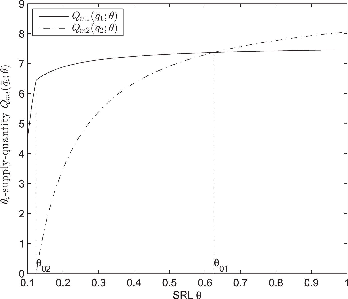
Effect of RCLC θ on θ-supply-quantity $Q_{mi} ({\bar{q}}_{i}; θ)$ .

Fig. 3

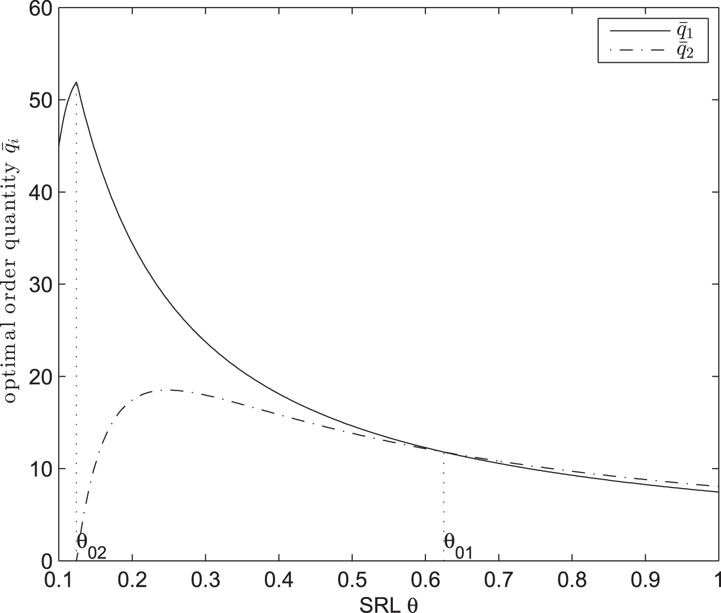
Effect of SRL θ on order quantity ${\bar{q}}_{i}$ .

3.3 Decentralized supply chain

Now we research the case that under the SRL θ_i, supplier i offers the retailer a wholesale price w_i per unit of successful delivery in a decentralized supply chain.

Under the SRL θ_i, the retailer’s profit can be written as

$\begin{matrix} v (q_{1}, q_{2}, w_{1}, w_{2}; θ_{1}, θ_{2}) = \\ \sum_{i = 1}^{2} (p_{i} (q_{1}, q_{2}; θ_{1}, θ_{2}) - w_{i}) Q_{mi} (q_{i}; θ_{i}) . \end{matrix}$ (3) Furthermore, supplier i’s profit can be denoted by $\begin{matrix} u_{i} (q_{i}, w_{i}; θ_{i}) = w_{i} Q_{mi} (q_{i}; θ_{i}) - c_{1 i} q_{i} - c_{2 i} Q_{mi} (q_{i}; θ_{i}) \\ = (w_{i} - c_{i}) Q_{mi} (q_{i}; θ_{i}) . \end{matrix}$ (4)

For convenience, we denote W_i = w_i - c_i and assume that the profit of supplier i is greater than or equal to zero. Eqs. (3) and (4) can be equivalently transformed into the following ones, $\begin{matrix} \begin{matrix} v (q_{1}, q_{2}, W_{1}, W_{2}; θ_{1}, θ_{2}) = \\ \sum_{i = 1}^{2} (p_{i} (q_{1}, q_{2}; θ_{1}, θ_{2}) - W_{i} - c_{i}) Q_{mi} (q_{i}; θ_{i}), \\ u_{i} (q_{i}, W_{i}; θ_{i}) = W_{i} Q_{mi} (q_{i}; θ_{i}) . \end{matrix} \end{matrix}$

Based on the previous point of view, the model for the decentralized supply chain is

${\begin{matrix} max_{W_{i} ⩾ 0} u_{i} ({\hat{q}}_{i}, W_{i}; θ_{i}) \\ subject to : \\ ({\hat{q}}_{1}, {\hat{q}}_{2}) = arg max_{q_{1}, q_{2} ⩾ 0} v (q_{1}, q_{2}, W_{1}, W_{2}; θ_{1}, θ_{2}) . \end{matrix}$ (5) In Model (5), the retailer and the suppliers maximize their own profits under the SRL θ_i. This means that if the retailer places an order of q_i units, then supplier i supplies Q_mi (q_i ; θ_i) units of the products under the SRL θ_i, and provides a price W_i to the retailer.

Lemma 2. The optimal order quantities ${\hat{q}}_{1}$ and ${\hat{q}}_{2}$ which satisfy the constrained conditions in Model (5) have the following characteristics.

(i) When W₂ ⩽ C₂ - (C₁ - W₁)/γ, we have $\begin{matrix} \begin{matrix} {\hat{q}}_{1} (W_{1}, W_{2}) = 0, {\hat{q}}_{2} (W_{1}, W_{2}) = (C_{2} - W_{2}) / (2 Φ_{2}^{- 1} (θ_{2})) . \end{matrix} \end{matrix}$ (ii) When C₂ - (C₁ - W₁)/γ < W₂ < C₂ - γ (C₁ - W₁), we have $\begin{matrix} \begin{matrix} {\hat{q}}_{1} (W_{1}, W_{2}) = \frac{(C_{1} - W_{1}) - γ (C_{2} - W_{2})}{(2 - 2 γ^{2}) Φ_{1}^{- 1} (θ_{1})}, \\ {\hat{q}}_{2} (W_{1}, W_{2}) = \frac{(C_{2} - W_{2}) - γ (C_{1} - W_{1})}{(2 - 2 γ^{2}) Φ_{2}^{- 1} (θ_{2})} . \end{matrix} \end{matrix}$ (iii) When C₂ - γ (C₁ - W₁) ⩽ W₂ ⩽ C₂, we have $\begin{matrix} \begin{matrix} {\hat{q}}_{1} (W_{1}, W_{2}) = (C_{1} - W_{1}) / (2 Φ_{1}^{- 1} (θ_{1})), {\hat{q}}_{2} (W_{1}, W_{2}) = 0 . \end{matrix} \end{matrix}$

Theorem 2. The equilibrium of the decentralized supply chain is as follows.

(i) If β < γ/2, we obtain $\begin{matrix} \begin{matrix} {\hat{q}}_{1} = 0, {\hat{q}}_{2} = C_{2} / (4 Φ_{2}^{- 1} (θ_{2})), {\hat{W}}_{1} \in [0, C_{1}], {\hat{W}}_{2} = C_{2} / 2, \\ {\hat{s}}_{1} = 0, {\hat{s}}_{2} = 3 C_{2}^{2} / 16, {\hat{s}}_{1} + {\hat{s}}_{2} = 3 C_{2}^{2} / 16 . \end{matrix} \end{matrix}$ (ii) If γ/2 ⩽ β ⩽ γ/(2 - γ²), we obtain $\begin{matrix} \begin{matrix} {\hat{q}}_{1} = 0, {\hat{q}}_{2} = C_{1} / (2 γ Φ_{2}^{- 1} (θ_{2})), {\hat{W}}_{1} = 0, {\hat{W}}_{2} = C_{2} - C_{1} / γ, \\ {\hat{s}}_{1} = 0, {\hat{s}}_{2} = C_{1} (2 γ C_{2} - C_{1}) / (4 γ^{2}), \\ {\hat{s}}_{1} + {\hat{s}}_{2} = C_{1} (2 γ C_{2} - C_{1}) / (4 γ^{2}) . \end{matrix} \end{matrix}$ (iii) If γ/(2 - γ²) < β < (2 - γ²)/γ, we obtain $\begin{matrix} \begin{matrix} {\hat{q}}_{i} = \frac{(2 - γ^{2}) C_{i} - γ C_{j}}{(2 - 2 γ^{2}) (4 - γ^{2}) Φ_{i}^{- 1} (θ_{i})}, {\hat{W}}_{i} = \frac{(2 - γ^{2}) C_{i} - γ C_{j}}{4 - γ^{2}}, \\ {\hat{s}}_{i} = \frac{[(6 - 2 γ^{2}) C_{i} - γ C_{j}] [(2 - γ^{2}) C_{i} - γ C_{j}]}{(4 - 4 γ^{2}) (4 - γ^{2})^{2}}, \\ {\hat{s}}_{1} + {\hat{s}}_{2} = \frac{\sum_{i = 1}^{2} [(6 - 2 γ^{2}) C_{i} - γ C_{j}] [(2 - γ^{2}) C_{i} - γ C_{j}]}{(4 - 4 γ^{2}) (4 - γ^{2})^{2}} . \end{matrix} \end{matrix}$ Especially when β = 1, we have $\begin{matrix} \begin{matrix} {\hat{q}}_{i} = C_{1} / [(2 + 2 γ) (2 - γ) Φ_{i}^{- 1} (θ_{i})], {\hat{W}}_{i} = (1 - γ) C_{1} / (2 - γ), \\ {\hat{s}}_{i} = (3 - 2 γ) C_{1}^{2} / [4 (1 + γ) (2 - γ)^{2}], \\ {\hat{s}}_{1} + {\hat{s}}_{2} = (3 - 2 γ) C_{1}^{2} / [2 (1 + γ) (2 - γ)^{2}] . \end{matrix} \end{matrix}$ (iv) If (2 - γ²)/γ ⩽ β ⩽ 2/γ, we obtain $\begin{matrix} \begin{matrix} {\hat{q}}_{1} = C_{2} / (2 γ Φ_{1}^{- 1} (θ_{1})), {\hat{q}}_{2} = 0, {\hat{W}}_{1} = C_{1} - C_{2} / γ, {\hat{W}}_{2} = 0, \\ {\hat{s}}_{1} = C_{2} (2 γ C_{1} - C_{2}) / (4 γ^{2}), {\hat{s}}_{2} = 0, \\ {\hat{s}}_{1} + {\hat{s}}_{2} = C_{2} (2 γ C_{1} - C_{2}) / (4 γ^{2}) . \end{matrix} \end{matrix}$ (v) If β > 2/γ, we obtain $\begin{matrix} \begin{matrix} {\hat{q}}_{1} = C_{1} / (4 Φ_{1}^{- 1} (θ_{1})), {\hat{q}}_{2} = 0, {\hat{W}}_{1} = C_{1} / 2, {\hat{W}}_{2} \in [0, C_{2}], \\ {\hat{s}}_{1} = 3 C_{1}^{2} / 16, {\hat{s}}_{2} = 0, {\hat{s}}_{1} + {\hat{s}}_{2} = 3 C_{1}^{2} / 16 . \end{matrix} \end{matrix}$

Theorem 2 implies that for any given competitive intensity, whether the market is monopolized by one channel depends on the two channels’ belief-degree costs, which reflect the supply uncertainty and the risk attitude of the retailer. When the difference in belief-degree costs between the two suppliers is significant enough (i.e., case (i) or (v)) or is significant (i.e., case (ii) or (iv)), the retailer only places an order from the supplier with a low belief-degree cost. In fact, β ⩽ γ/(2 - γ²) and γ ∈ [0, 1] mean that supplier 2’s belief-degree cost is far lower than that of supplier 1, whereas β ⩾ (2 - γ²)/γ denotes that his belief-degree cost is far higher than that of supplier 1. Thus, the first, second, fourth or fifth conclusion shows that only the supplier with a sufficiently low belief-degree cost supplies the products to the retailer. When the difference in belief-degree costs is not significant (i.e., case (iii)), the retailer orders the products from the two suppliers.

Similar to the analysis of the integrated game, we first consider a special case where there is no supply uncertainty (i.e., $Φ_{1}^{- 1} (θ_{1}) = 1$ or θ = 1), the two products are perfect substitutes (γ = 1), and their costs are the same (i.e., C₁ = C₂ = C). In this case, the retailer only places an order of C/2 from either of the two channels, and the profit of the entire supply chain is C²/4; these findings are consistent with the classical results. Second, in our settings, the supply uncertainty described by the distribution Φ_i and the risk attitude of the retailer described by the SRL θ_i are reflected in the belief-degree cost of channel i described by c_i. That is, the retailer believes that for given SRLs θ₁ and θ₂, the channel with a lower belief-degree cost should supply more products to the market because it can decrease the purchase cost of the retailer and then increase her profits. If the belief-degree cost of a channel is sufficiently low, then the products being fully supplied by this channel can maximize the profit of the retailer.

The impact of the SRL on the θ_i-supply-quantity and the profits of channel i can be seen from the following proposition.

Proposition 5. For the decentralized supply chain, when the difference in belief-degree costs between the two suppliers is significant enough, both the θ_i-supply-quantity and the channel profits are increasing with the corresponding SRL. When the difference in belief-degree costs is significant, the θ_i-supply-quantity of one channel increases with the competitive channel’s SRL. The channel profit increases with both its own and its competitive channel’s SRLs. When the difference in belief-degree costs is not significant, the channel with a lower belief-degree cost gains a competing advantage in θ_i-supply-quantity and profits, i.e.,

When γ/(2 - γ²) < β < 1, channel 2 gains a competitive advantage in θ_i-supply-quantity and profits over channel 1 (i.e., $Q_{m 2} ({\hat{q}}_{2}; θ_{2}) > Q_{m 1} ({\hat{q}}_{1}; θ_{1})$ and ${\hat{s}}_{2} > {\hat{s}}_{1}$ ).

When β = 1, the two channels reach balance in θ_i-supply-quantity and profits (i.e., $Q_{m 2} ({\hat{q}}_{2}; θ_{2}) = Q_{m 1} ({\hat{q}}_{1}; θ_{1})$ and ${\hat{s}}_{2} = {\hat{s}}_{1}$ ).

When 1 < β < (2 - γ²)/γ, channel 1 gains a competitive advantage in θ_i-supply-quantity and profits over channel 2 (i.e., $Q_{m 2} ({\hat{q}}_{2}; θ_{2}) < Q_{m 1} ({\hat{q}}_{1}; θ_{1})$ and ${\hat{s}}_{2} < {\hat{s}}_{1}$ ).

Moreover, both the θ_i-supply-quantity and profits of channel i are increasing in θ_i, and decreasing in θ_j. Specifically, they are decreasing in γ when β = 1.

Similar to the analysis of the integrated game, Proposition 5 demonstrates the impact of the retailer’s attitudes toward the supply risks on the market supply and the profits of the channels. The belief-degree cost of one channel is only affected by the supply risk attitude of the retailer when the production and successful delivery costs and the distributions of the uncertain supply ratios are given. Therefore, if the retailer has different risk attitudes toward the supply uncertainty of the two channels, then there is a difference between the belief-degree costs of the two channels. When this difference is significant enough, the market is monopolized by the channel with a sufficiently low belief-degree cost. Moreover, in this case, the market supply and profit of the retailer from this channel are not affected by her attitude toward its competing channel’s supply risk because the difference between the belief-degree costs of the two channels is significant enough. An adventurous retailer prefers to adopt the order strategy that generates greater market supply to obtain more profits despite increasing her purchasing cost. Conversely, a conservative retailer may adopt the order strategy that generates less market supply and obtain less profits despite decreasing her purchasing cost.

When the difference is significant, the market is still monopolized by the channel with a sufficiently low belief-degree cost. In this case, the market supply and profit of the retailer from this channel are affected by her attitude toward its competing channel’s supply risk. In fact, although the difference between the belief-degree costs of the two channels is significant, the difference is lower than in the above case. Thus, the retailer’s attitude toward its competitive channel’s supply risk directly affects the purchasing cost from this channel and then affects the market supply and profit from this channel. Moreover, the market supply and profit from this channel increase if the retailer’s attitude toward its competitive channel’s supply risk shifts from averse to loving because the purchasing cost of the retailer from this channel decreases in this case. This conclusion is counterintuitive because in the next case, we show that an increase in the competitive channel’s SRL decreases the market supply and profit from this channel. However, it is reasonable because in this case, the market supply is monopolized by this channel due to the significant difference between the belief-degree costs of the two channels; an increase in the competitive channel’s SRL decreases the purchasing cost from this channel and then increases the market supply from this channel to obtain more profits.

When a change in the retailer’s risk attitude makes the difference in belief-degree costs non-significant, the retailer is willing to provide more market supply from the channel with a lower belief-degree cost to obtain more profits. Furthermore, if the attitude of the retailer is loving to the supply risk of this channel or averse to that of the other channel, then the profit of this channel increases because the market supply from this channel increases. This conclusion is intuitive because an adventurous decision maker may obtain more profit by providing more market supply. If the retailer is averse to the supply risk of this channel’s competitor, the retailer will decrease the market supply from the competing channel and then increase the market supply from this channel.

The impact of the SRL on the order strategy of the retailer can be seen from the following proposition.

Proposition 6. For the decentralized supply chain, when the difference in belief-degree costs between the two channels is significant enough, the order quantity of the retailer from a lower belief-degree cost’s channel decreases in θ_i if $Φ_{i}^{- 1} (θ_{i}) > 2 c_{1 i} / (A - c_{2 i})$ ; otherwise, it increases in θ_i. When the difference in belief-degree costs is significant, the order quantity of the retailer from the channel with a lower belief-degree cost decreases with its SRL and the competitive intensity, while increases with its competitive channel’s SRL. When the difference in belief-degree costs is not significant, the order quantity of the retailer from channel i decreases in θ_i if $Φ_{i}^{- 1} (θ_{i}) > 2 c_{1 i} / [A - c_{2 i} - γ C_{j} / (2 - γ^{2})]$ ; otherwise, it increases in θ_i, and decreases in θ_j. The comparison of her order quantities from the two channels is as follows.

When $[(2 - γ^{2}) β - γ] / Φ_{1}^{- 1} (θ_{1}) = (2 - γ^{2} - β γ) / Φ_{2}^{- 1} (1 - θ_{2})$ , the order quantities of the retailer from the two channels reach balance (i.e., ${\hat{q}}_{1} = {\hat{q}}_{2}$ ). Specifically, when β = 1 and $Φ_{1}^{- 1} (θ_{1}) = Φ_{2}^{- 1} (θ_{2})$ , the two order quantities are the same (i.e., ${\hat{q}}_{1} = {\hat{q}}_{2}$ ).

When $[(2 - γ^{2}) β - γ] / Φ_{1}^{- 1} (θ_{1}) > (2 - γ^{2} - β γ) / Φ_{2}^{- 1} (θ_{2})$ , the retailer orders more units of the products from channel 1 than from channel 2 (i.e., ${\hat{q}}_{1} > {\hat{q}}_{2}$ ). Otherwise, the order quantity from channel 1 is less than that from channel 2 (i.e., ${\hat{q}}_{1} < {\hat{q}}_{2}$ ).

Proposition 6 describes the impact of the retailer’s attitudes toward the supply risks of the two channels on the order strategy. We only analyze the case in which the difference in belief-degree costs between the two channels is significant and the analyses of the other cases are similar to those of the integrated game. When the difference in the retailer’s supply risk attitudes toward the two channels causes the belief-degree costs of the two channels to be significantly different, the market is monopolized by the channel with a sufficiently low belief-degree cost. The order quantity of the retailer from this monopolistic channel decreases with the SRL of this channel and the competitive intensity, while increases with its competitive channel’s SRL. This result is reasonable and the explanation is as follows. An increase in the competitive channel’s SRL implies that a market supply from this monopolistic channel increases by Proposition 5. And in this channel, the market supply is the product of the order quantity and the supply ratio of this channel, that is, the order quantity is the ratio of the market supply from this channel to its supply ratio. Whereas the market supply from this channel increases with its competitor’s SRL and decreases with the competitive intensity. The supply ratio of this channel increases with its own SRL. Therefore, the order quantity of the retailer from the monopolistic channel decreases as the SRL of this channel or the competitive intensity, and increases as its competitive channel’s SRL.

Proposition 7. For the decentralized supply chain, when the difference in belief-degree costs is not significant, the total θ_i-supply-quantity $Q_{m 1} ({\hat{q}}_{1}; θ_{1}) + Q_{m 2} ({\hat{q}}_{2}; θ_{2}) = (C_{1} + C_{2}) / (2 + 2 γ) (2 - γ)$ , which is increasing in θ₁, θ₂ and decreases in γ.

Proposition 7 implies that a risk-loving retailer prefers to adopt the order strategy that provides more total market supply to obtain a larger profit because she believes that the belief-degree cost of each of the two channels is lower, whereas a risk-averse retailer prefers to provide less total market supply. Moreover, intense competition decreases the total market supply.

The parameter β is increasing in θ₁, while is decreasing in θ₂. Therefore, we derive the following proposition.

Proposition 8. For the decentralized supply chain, when the SRL θ₁ increases or θ₂ decreases, channel 1 possesses a competing advantage in θ_i-supply-quantity and profits over channel 2, and vice versa.

Proposition 8 implies that the retailer can adjust the market supply and the profits of each channel by adjusting her attitude toward supply risk of each channel. When the retailer’s attitudes toward the supply risks of the two channels induce the belief-degree costs of the two channels to be no difference, the market supplies and profits of the two channels are the same. If the retailer believes that the supply uncertainty of a channel is low (or that of its competitive channel is high), then the SRL of this channel (or its competitive channel) may increase (or decrease). As a result, its (or its competitive channel’s) belief-degree cost decreases (or increases), and thus, there is a difference between the two belief-degree costs. Both the market supply and profits of this channel are higher than those of its competitive channel if the difference is not significant (i.e., γ/(2 - γ²) < β < (2 - γ²)/γ); otherwise, this channel monopolizes the market.

A numerical analysis discusses the effect of the SRLs θ₁ and θ₂ on the θ_i-supply-quantities and the order quantities of the two channels (see Figs. 4 and 5, where $ξ_{i} \sim L (0, 1), A = 30, c_{11} = 2, c_{21} = 1, c_{12} = 2.5, c_{22} = 0.2, θ_{2} = 0.5$ and γ = 3/4). In Fig. 4, the SRL θ₁ = θ₀₁ is such that $Q_{m 1} ({\hat{q}}_{1}; θ_{1}) = Q_{m 2} ({\hat{q}}_{2}; θ_{2})$ , and θ₁ = θ₀₂ is a threshold distinguishing whether the retailer orders the products from one or two supplier(s). Similarly, the SRL θ₁ = θ₀₁ or θ₀₂ is such that ${\hat{q}}_{1} = {\hat{q}}_{2}$ , and θ₁ = θ₀₃ is a threshold distinguishing whether the retailer orders the products from one or two supplier(s) in Fig. 5. From Fig. 4, we observe that as the SRL decreases, the θ₁-supply-quantity of channel 1 decreases. However, the θ₂-supply-quantity of channel 2 increases if θ₁ > θ₀₂, and decreases if θ₁ < θ₀₂ which corresponds case (ii) in Theorem 2. Moreover, when the SRL is higher (i.e., θ₁ > θ₀₁), supplier 1 supplies more units of the products under the SRL θ₁, otherwise, the θ₂-supply-quantity of supplier 2 is more. From Fig. 5, we observe that there exist two values θ₀₁ and θ₀₂ of the SRL such that the equation ${\hat{q}}_{1} = {\hat{q}}_{2}$ holds. If θ₁ > θ₀₁ or θ₁ < θ₀₂, the retailer orders more units of the products from supplier 2 than from supplier 1. Otherwise, the order quantity from supplier 1 is more than that from supplier 2. In addition, if θ₁ > θ₀₃, implying that the retailer places orders from both the suppliers, the order quantity of channel 1 firstly increases and then decreases with respect to the SRL θ₁, whereas supplier 2’s order quantity decreases in θ₁. If θ₁ < θ₀₃, supplier 2 is in the monopoly position and it is good for him when his competitive supplier’s supply risk level increases. Simultaneously observing the two figures, we find that in the decentralized supply chain, the higher the SRL, the more intense the competition between the two suppliers. Conversely, the supply market is monopolized by the supplier with the lower belief-degree cost. Similar to Figs. 2 and 3, Figs 4 and 5 also imply that the competition between the two suppliers exits in the supply market with the higher SRLs.

Fig. 4

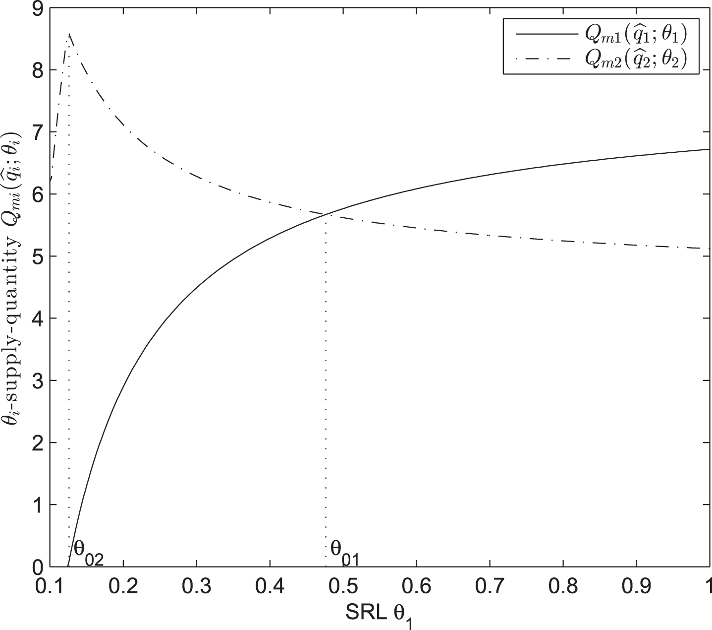
Effect of SRL θ₁ on θ_i-supply-quantity $Q_{mi} ({\hat{q}}_{i}; θ_{i})$ .

Fig. 5

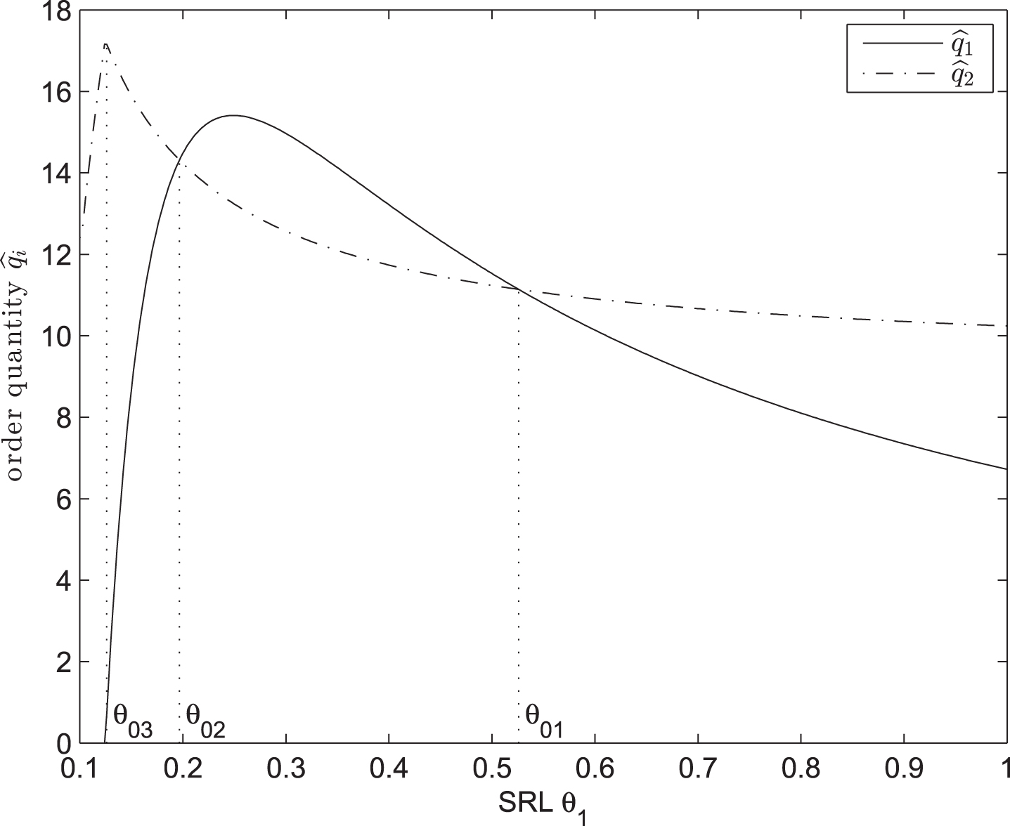
Effect of SRL θ₁ on order quantity ${\hat{q}}_{i}$ .

4 Strategy comparison

Under the SRL α_i, this section compares the order quantities, θ_i-supply-quantities, market clearing prices, and profits of the channels and total supply chains in the integrated and decentralized supply chains. We perform the comparisons only for the case in which the retailer places orders from both channels (i.e., the case γ < β < 1/γ). By the second conclusion in Theorem 1 and the third conclusion in Theorem 2, we obtain the following four propositions.

Proposition 9. When the retailer places orders from both suppliers, we have $Q_{m 1} ({\hat{q}}_{1}; θ_{1}) + Q_{m 2} ({\hat{q}}_{2}; θ_{2}) ⩽ Q_{m 1} ({\bar{q}}_{1}; θ_{1}) + Q_{m 2} ({\bar{q}}_{2}; θ_{2})$ ; and ${\hat{q}}_{1} + {\hat{q}}_{2} < {\bar{q}}_{1} + {\bar{q}}_{2}$ if $β > [γ (3 - γ^{2}) Φ_{2}^{- 1} (θ_{2}) - 2 Φ_{1}^{- 1} (θ_{1})] / [2 Φ_{2}^{- 1} (θ_{2}) - γ (3 - γ^{2}) Φ_{1}^{- 1} (θ_{1})]$ , otherwise, ${\hat{q}}_{1} + {\hat{q}}_{2} ⩾ {\bar{q}}_{1} + {\bar{q}}_{2}$ . The order quantities and the θ_i-supply-quantities in each channel have the following characteristics.

If γ < β < γ (3 - γ²)/2, where γ (3 - γ²)/2 ∈ [0, 1], then ${\hat{q}}_{1} > {\bar{q}}_{1}, {\hat{q}}_{2} < {\bar{q}}_{2}$ and $Q_{m 1} ({\hat{q}}_{1}; θ_{1}) > Q_{m 1} ({\bar{q}}_{1}; θ_{1}), Q_{m 2} ({\hat{q}}_{2}; θ_{2}) < Q_{m 2} ({\bar{q}}_{2}; θ_{2})$ ;

If γ (3 - γ²)/2 < β < 2/[γ (3 - γ²)], then ${\hat{q}}_{1} < {\bar{q}}_{1}, {\hat{q}}_{2} < {\bar{q}}_{2}$ and $Q_{m 1} ({\hat{q}}_{1}; θ_{1}) < Q_{m 1} ({\bar{q}}_{1}; θ_{1})$ , $Q_{m 2} ({\hat{q}}_{2}; θ_{2}) < Q_{m 2} ({\bar{q}}_{2}; θ_{2})$ ;

If 2/[γ (3 - γ²)] < β < 1/γ, then ${\hat{q}}_{1} < {\bar{q}}_{1}, {\hat{q}}_{2} > {\bar{q}}_{2}$ and $Q_{m 1} ({\hat{q}}_{1}; θ_{1}) < Q_{m 1} ({\bar{q}}_{1}; θ_{1}), Q_{m 2} ({\hat{q}}_{2}; θ_{2}) > Q_{m 2} ({\bar{q}}_{2}; θ_{2})$ .

Proposition 9 reveals that for a given SRL θ_i in the integrated and decentralized games, when there is competition in the supply market, the total market supply in the decentralized supply chain is no more than that in the integrated supply chain, which is consistent with the classical result that integration dominates decentralization as a strategy. Here, the result is more general for cases in which different SRLs are considered. The total order quantity in the decentralized game is the same or lower than that in the integrated game if the difference in belief-degree costs between the two channels is greater; otherwise, the total order quantity is greater in the decentralized game. The finding is reasonable, and the explanation is as follows. Different attitudes toward the supply risks of the two channels cause a difference in belief-degree costs between the two channels and a difference in supply ratios between the two channels. These two differences allow the total order quantity in the decentralized game to be smaller or greater than that in the integrated game, although the total market supply in the former game is less than that in the latter game.

Moreover, if the difference in belief-degree costs between the two channels is greater (i.e., case (i) or (iii)), the order quantity and the θ_i-supply-quantity of the channel with a lower belief-degree cost in the decentralized supply chain are less than those in the integrated supply chain, whereas those of the other channel in the decentralized supply chain are greater. However, if the difference in belief-degree costs between the two channels is smaller (i.e., case (ii)), both quantities in the decentralized supply chain are less than those in the integrated supply chain. Under the assumptions of our study, there is no situation in which both quantities in the decentralized supply chain are greater than those in the integrated supply chain. These conclusions imply that integration is a better strategy under different SRLs.

Fig. 6 illustrates the comparison between the order quantities in the integrated and decentralized supply chains when the parameter β reflecting the difference in belief-degree costs changes with the competition intensity γ. From Fig. 6, we observe that the first, second and third areas are corresponding to cases (i), (ii) and (iii) in Proposition 9, respectively. When β > 1/γ or β < γ (i.e., in the fourth or fifth area), the case represents that there is one monopolistic supply market at least in the decentralized and integrated supply chains.

Fig. 6

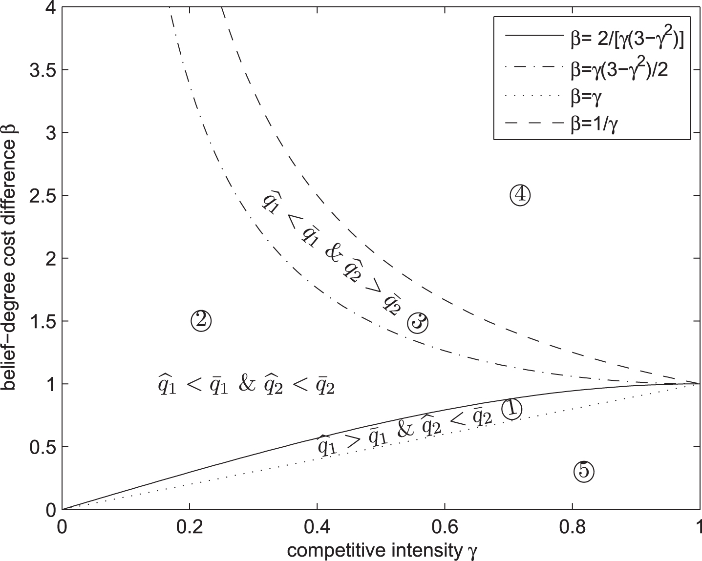
Comparison of supply chain’s order quantities.

Proposition 10. When the retailer places orders from both suppliers, the total profit in the decentralized supply chain is no higher than in the integrated supply chain (i.e., ${\hat{s}}_{1} + {\hat{s}}_{2} ⩽ {\bar{s}}_{1} + {\bar{s}}_{2}$ ). The channel profits have the following characteristics.

If γ < β < β₁ (γ), where $β_{1} (γ) = ((8 γ - 5 γ^{3} + γ^{5}) + (4 γ - γ^{3}) \sqrt{5 - 2 γ^{2} + γ^{4}}) / (8 + 4 γ^{2} - 2 γ^{4})$ ∈[0, 1], then ${\hat{s}}_{1} > {\bar{s}}_{1}$ and ${\hat{s}}_{2} < {\bar{s}}_{2}$ ;

If β₁ (γ) < β < 1/β₁ (γ), then ${\hat{s}}_{1} < {\bar{s}}_{1}$ and ${\hat{s}}_{2} < {\bar{s}}_{2}$ ;

If 1/β₁ (γ) < β < 1/γ, then ${\hat{s}}_{1} < {\bar{s}}_{1}$ and ${\hat{s}}_{2} > {\bar{s}}_{2}$ .

Similar to the analysis of Proposition 9, Proposition 10 reveals that the total profit in the decentralized supply chain is no higher than that in the integrated supply chain. For any given competitive intensity, when the difference in belief-degree costs is greater, the profit of the channel with a lower belief-degree cost in the decentralized supply chain is lower than that in the integrated supply chain, whereas that of the other channel is higher in the decentralized supply chain. When the difference in belief-degree costs is smaller, both channels’ profits are higher in the integrated supply chain. There is no case in which the two channels’ profits are both higher in the decentralized supply chain.

Propositions 9 and 10 imply that from the perspectives of the θ_i-supply-quantities, the order quantities and the channel profits are compared under integration and decentralization. When the difference in belief-degree costs is greater, the channel with a higher belief-degree cost in the integrated supply chain is dominated by that in the decentralized supply chain, whereas we have the opposite conclusion for the other channel. However, when the difference in belief-degree costs is smaller, the three parameters of the two channels in the decentralized supply chain are dominated by those in the integrated supply chain. This conclusion reveals that the decision maker of the channel with a higher belief-degree cost prefers the decentralization strategy when the difference in belief-degree costs between the two channels is greater. This result is reasonable because, in the decentralized supply chain, any decrease or increase of the total supply chain profit is due primarily to the decrease or increase of the profits of the channel with the lower belief-degree cost, in contrast to the case of an integrated supply chain.

Proposition 11. In the decentralized supply chain, when the retailer places orders from both suppliers, the market clearing price of the products sold through channel i is higher than that in the integrated supply chain (i.e., $p_{i} ({\hat{q}}_{1}, {\hat{q}}_{2}; θ_{1}, θ_{2}) > p_{i} ({\bar{q}}_{1}, {\bar{q}}_{2}; θ_{1}, θ_{2})$ ).

Proposition 11 demonstrates that in the decentralized supply chain, the market clearing price of the products in each channel is higher than that in the integrated supply chain.

From Propositions 9 and 11, we know that under different SRLs, the integration strategy provides a better service to customers than the decentralization strategy because the customers benefit in the former case from greater total market supply and lower market clearing prices.

Proposition 12. For the decentralized supply chain, the range of the interval around β, on the basis of which the retailer places orders from the two suppliers, is wider than that in the integrated supply chain.

Proposition 12 shows that when there is competition in the supply market, the condition on the difference in belief-degree costs is relaxed in the decentralized supply chain as opposed to that in the integrated supply chain. In other words, in the decentralized supply chain with supply uncertainty, the competition between both channels is more intense in the integrated supply chain than in the decentralized supply chain.

5 Selection of risk preferences

The suppliers and the retailer do not know what the SRLs are in advance due to supply uncertainty. In real life, the SRLs are generally determined based on risk preferences of the central planner or the retailer to determine the order quantities of both channels. From Theorems 1 and 2, we know that if the SRLs of both channels are higher, then the supply chain’s total profit is higher in the integrated game, or the retailer earns a higher total profit in the decentralized game. Conversely, the lower SRLs signify lower profits. Theoretically, each choice of SRLs is not bad but is also not optimal (i.e., a non-inferior solution) from the perspective of both SRLs and profits. Therefore, the SRL being taken as 0.5 is an intermediate choice, which means that the supply quantity is the expected supply. However, in the following subsections, we consider how the central planner or retailer chooses suitable SRLs from the perspective of order quantities, which implies that the neutral attitude toward risk might not be the optimal choice for a rational decision maker.

5.1 The integrated case

In this subsection, the proper SRLs can be determined through jointly analyzing the effects of supply reliability and supply risk. Take case (i) in Theorem 1 as an example: When the SRL θ₂ decreases, supply reliability increases, which results in $1 / Φ_{2}^{- 1} (θ_{2})$ increasing, and then the order quantity ${\bar{q}}_{2}$ increases. However, the supply risk decreases (i.e., supply reliability increases), meaning that C₂ decreases, and that ${\bar{q}}_{2}$ decreases. In other words, an increase in supply reliability forces the order quantity to increase, whereas a decrease in supply risk forces the order quantity to decrease. Therefore, in the integrated case, when there is no more information to infer specific SRLs, the central planner can maximize the order quantities to strike a balance between supply reliability and risk. Following from Proposition 2, the proposition below is obtained.

Proposition 13. In order to maximize the order quantity of channel i about the SRL θ_i, we have

When the difference in belief-degree costs between the two suppliers is significant, the SRL θ_i satisfies the equation $Φ_{i}^{- 1} (θ_{i}) = min {2 c_{1 i} / (A - c_{2 i}), 1}$ .

When the difference in belief-degree costs between the two suppliers is not significant, the SRL θ_i satisfies the equation $Φ_{i}^{- 1} (θ_{i}) = min {(4 - γ^{2}) c_{1 i} / [(1 - γ) (2 + γ) A - (2 - γ^{2}) c_{2 i} + γ c_{2 j}], 1}$ .

Proposition 13 implies that there is a proper SRL such that the order quantity of supplier i is maximized in the integrated case. For example, when $ξ_{i} \sim L (0, 1), A = 30, c_{11} = 2, c_{21} = 1, c_{12} = 2.5, c_{22} = 0.2$ and γ = 3/4, we obtain that θ₁ = 0.3448 and θ₂ = 0.4310 by case (ii) in Proposition 13. Therefore, the central planner chooses the two channels’ SRLs 0.3448 and 0.4310, respectively, and the order quantities of both channels are 6.6286. In other words, the central planner chooses the SRLs under which channels 1 and 2 supply 6.6286 units of the products with the SRL of not more than 0.3448 and 0.4310 to the market, respectively. This result implies that the expected supply is not always appropriate.

5.2 The decentralized case

Similarly, the following proposition can be obtained in view of Proposition 6.

Proposition 14. In order to maximize the order quantity of channel i about the SRL θ_i, we have

When the difference in belief-degree costs between the two suppliers is significant enough, the SRl θ_i is solved by the equation $Φ_{i}^{- 1} (θ_{i}) = min {2 c_{1 i} / (A - c_{2 i}), 1}$ .

When the difference in belief-degree costs between the two suppliers is not significant, the SRL θ_i is solved by the equation $Φ_{i}^{- 1} (θ_{i}) = min {[(4 - 2 γ^{2})^{2} - γ^{2}] c_{1 i} / [(2 - γ^{2} - γ) (4 - 2 γ^{2} + γ) A - (2 γ^{4} - 7 γ^{2} + 8) c_{2 i} + γ (2 - γ^{2}) c_{2 j}], 1}$ .

Proposition 14 means that there is an ideal SRL such that the retailer’s order quantity from supplier i is maximized in the decentralized case. When the parameter values are the same as those in the integrated case, we obtain that θ₁ = 0.2165 and θ₂ = 0.2707 by case (ii) in Proposition 14. The SRLs in the decentralized case are lower than in the integrated case, respectively. This conclusion is also obtained theoretically by comparing Proposition 2 with Proposition 6. And the same supply quantity of the two channels is 4.5174. This result implies that to achieve the goal of maximizing the order quantities, the SRL and market supply of each channel in the decentralized case are lower than those in the integrated case, and then the market supply of each channel in the decentralized case is lower. That is, the decision maker’s attitude toward the supply uncertainty of each channel in the decentralized game should be more conservative than that in the integrated game. This result is reasonable, and the explanation is as follows. Because of the double marginal utility, the point at which the change rate of the order quantity about the SRL is zero in the decentralized case is distorted downward, compared with the centralized case (because 2c_1i/[A - c_2i - γC_j] >2c_1i/[A - c_2i - γC_j/(2 - γ²)] in Propositions 2 and 6). Therefore, the SRL of each channel in the decentralized case is lower than that in the centralized case, as a result, the market supply of each channel is lower in the decentralized case because the market supply of each channel decreases as the SRL decreases.

6 Managerial implications and conclusion

This paper considers an order problem of two channels composed of one common retailer and two suppliers subjected to supply uncertainty. Different from the relevant literature, a decision rule based on confidence level is proposed to measure the uncertain supply quantities of the two channels and study the optimal order strategy for two channels under different supply risk levels. There are three main managerial implications from the analytical results. First, in the absence of adequate data of supply uncertainty, the decision makers of two channels can estimate the distributions of supply uncertainty variables based on relevant experts to alleviate the uncertain risks. Second, for given distributions of uncertain variables, the risk attitudes of decision makers toward supply uncertainties give rise to the difference between the belief-degree costs of the two channels, which directly influences the optimal order strategy, market supply and profit of each channel. This implies that the decision makers can adopt different risk attitudes toward the supply uncertainty of the two channels to adjust the potential market supply and profit of each channel. Third, the SRLs suggested in Section 5 are lower in the decentralized case than in the centralized case, which shows that the decision maker’s risk attitude toward supply uncertainty of each channel should be more conservative in the decentralized case. This is intuitive, because in the centralized situation, the supplier and retailer are a whole, meaning that the decision maker’s judgment on the degree of supply uncertainty should be more accurate than that of the supplier and retailer operating independently.

In this paper, we only discuss the maximization problem of the profit under different supply risk levels. Considering both return maximization and risk minimization problems remains for future research. In addition, we only study the symmetric case in which the two suppliers and retailer know the distributions of uncertain supplies, all kinds of costs and risk attitudes of all participants. Future work can explore information asymmetry. These research topics would expand the scope of the literature on supply chain competition with information uncertainty.

Footnotes

Appendix

Proof of Lemma 1. The following lemma will be used in the proof of this theorem.

Lemma 3. [21] Let the function g (x, x₁, x₂, …, x_n) be strictly increasing with x₁, x₂, …, x_k and be strictly decreasing with x_k+1, x_k+2, …, x_n. If ξ₁, ξ₂, …, ξ_n are uncertain variables with uncertainty distributions Φ₁, Φ₂, …, Φ_n, respectively, then the chance constraint $M {g (x, ξ_{1}, ξ_{2}, \dots, ξ_{n}) ⩽ 0} ⩾ α$ holds if and only if $g (x, Φ_{1}^{- 1} (α), \dots, Φ_{k}^{- 1} (α), Φ_{k + 1}^{- 1} (1 - α), \dots, Φ_{n}^{- 1} (1 - α)) ⩽ 0,$ where 0 ⩽ α ⩽ 1.

By Lemma 3, the chance constraint $M {ξ_{i} q_{i} ⩾ Q_{0 i}} ⩾ 1 - θ_{i}$ is equivalent to $Q_{0 i} - Φ_{i}^{- 1} (θ_{i}) q_{i} \leq 0 .$ Thus, supplier i’s θ_i-supply-quantity $Q_{mi} (q_{i}; θ_{i}) = max {Q_{0 i}} = Φ_{i}^{- 1} (θ_{i}) q_{i}$ . This completes the proof of the lemma.

Proof of Theorem 1. Since the objective function in Model (2) is concave about the order quantity q_i, its first-order conditions are $2 Φ_{i}^{- 1} (θ_{i}) q_{i} + 2 γ Φ_{j}^{- 1} (θ_{j}) q_{j} = C_{i} .$ Solving it, the conclusions in Theorem 1 can be obtained. This completes the proof of the theorem.

Proofs of Propositions 1, 2 and 3. Propositions 1, 2 and 3 can be obtained by Theorem 1.

Proof of Lemma 2. Model (5) can be equivalently transformed into the following one,

(6) ${\begin{matrix} max_{W_{i} ⩾ 0} u_{i} ({\hat{q}}_{i}, W_{i}; α_{i}) = max_{W_{i} ⩾ 0} W_{i} Φ_{i}^{- 1} (θ_{i}) {\hat{q}}_{i} \\ subject to : \\ 2 Φ_{i}^{- 1} (θ_{i}) {\hat{q}}_{i} + 2 γ Φ_{j}^{- 1} (θ_{j}) {\hat{q}}_{j} = C_{i} - W_{i} \\ 2 Φ_{j}^{- 1} (θ_{j}) {\hat{q}}_{j} + 2 γ Φ_{i}^{- 1} (θ_{i}) {\hat{q}}_{i} = C_{j} - W_{j} \\ {\hat{q}}_{i}, {\hat{q}}_{j} \geq 0 . \end{matrix}$ We solve the equation set in (6) about the variables ${\hat{q}}_{i}$ and ${\hat{q}}_{j}$ , and then substitute ${\hat{q}}_{i}$ into the objective function. And thus, the objective function is concave about W_i, and the lemma can be proved by solving the problem of maximizing the suppliers’ profits only including the constrained condition W_i ⩾ 0.

Proof of Theorem 2. We first derive the best-response function of W₂ for any given W₁ from the following three cases.

Case 1: If C₂ < γ (C₁ - W₁), i.e., W₁ < C₁ - C₂/γ, we only need to consider situation (iii) in Lemma 2. We obtain W₂ can be any value on the interval [0, C₂], $q_{1} = (C_{1} - W_{1}) / (2 Φ_{1}^{- 1} (θ_{1})), q_{2} = 0$ .

Case 2: If γ (C₁ - W₁) ⩽ C₂ < (C₁ - W₁)/γ, i.e., C₁ - C₂/γ ⩽ W₁ < C₁ - γC₂, we need to consider situations (ii) and (iii) in Lemma 2.

By situation (ii) in Lemma 2, the objective function in Model (6) is $\begin{matrix} \begin{matrix} max_{W_{2} ⩾ 0} u_{2} ({\hat{q}}_{2}, W_{2}; θ_{2}) = \\ max_{W_{2} ⩾ 0} {W_{2} \frac{(C_{2} - W_{2}) - γ (C_{1} - W_{1})}{2 - 2 γ^{2}}} . \end{matrix} \end{matrix}$ Its first-order condition is W₂ = C₂/2 - γ (C₁ - W₁)/2, which satisfies the condition C₂ - (C₁ - W₁)/γ < W₂ < C₂ - γ (C₁ - W₁). Thus, the optimal order quantity and the maximum profit are $\begin{matrix} \begin{matrix} q_{2} = \frac{C_{2} - γ (C_{1} - W_{1})}{(4 - 4 γ^{2}) Φ_{2}^{- 1} (θ_{2})}, u_{2} = \frac{[C_{2} - γ (C_{1} - W_{1})]^{2}}{8 - 8 γ^{2}} . \end{matrix} \end{matrix}$ Since the maximum profit of supplier 2 under situation (iii) in Lemma 2 is zero, it is clear that situation (ii) is better, which implies that if C₁ - C₂/γ < W₁ < C₁ - γC₂ (i.e., γ (C₁ - W₁) < C₂ < (C₁ - W₁)/γ), we have $\begin{matrix} \begin{matrix} W_{2} = \frac{C_{2}}{2} - \frac{γ (C_{1} - W_{1})}{2}, q_{2} = \frac{C_{2} - γ (C_{1} - W_{1})}{(4 - 4 γ^{2}) Φ_{2}^{- 1} (θ_{2})}, \\ u_{2} = \frac{[C_{2} - γ (C_{1} - W_{1})]^{2}}{8 - 8 γ^{2}} . \end{matrix} \end{matrix}$

Case 3: If C₂ ⩾ (C₁ - W₁)/γ, i.e., W₁ ⩾ C₁ - γC₂, we need to consider situations (i), (ii) and (iii) in Lemma 2.

•By situation (i) in Lemma 2, the objective function in Model (6) $\begin{matrix} \begin{matrix} max_{W_{2} ⩾ 0} u_{2} ({\hat{q}}_{2}, W_{2}; θ_{2}) = max_{W_{2} ⩾ 0} {W_{2} \frac{C_{2} - W_{2}}{2}} . \end{matrix} \end{matrix}$ Its first-order condition is W₂ = C₂/2, then there are two subcases.

· If C₂/2 > (C₁ - W₁)/γ, then $W_{2} = C_{2} / 2, q_{2} = C_{2} / (4 Φ_{2}^{- 1} (θ_{2})), u_{2} = C_{2}^{2} / 8$ .

· If C₂/2 ⩽ (C₁ - W₁)/γ, then $W_{2} = C_{2} - (C_{1} - W_{1}) / γ, q_{2} = (C_{1} - W_{1}) / (2 γ Φ_{2}^{- 1} (θ_{2})), u_{2} = (C_{1}$ -W₁) [C₂ - (C₁ - W₁)/γ]/(2γ).

•By situation (ii) in Lemma 2, the objective function in Model (6) is $\begin{matrix} \begin{matrix} max_{W_{2} ⩾ 0} u_{2} ({\hat{q}}_{2}, W_{2}; θ_{2}) = \\ max_{W_{2} ⩾ 0} {W_{2} \frac{(C_{2} - W_{2}) - γ (C_{1} - W_{1})}{2 - 2 γ^{2}}} . \end{matrix} \end{matrix}$ Its first-order condition is W₂ = [C₂ - γ (C₁ - W₁)]/2, then there are two subcases.

· If [C₂ - γ (C₁ - W₁)]/2 > C₂ - (C₁ - W₁)/γ, i.e., C₂/2 < (2 - γ²) (C₁ - W₁)/(2γ), then W₂ = [C₂ - γ (C₁ - W₁)]/2, $q_{2} = [C_{2} - γ (C_{1} - W_{1})] / [(4 - 4 γ^{2}) Φ_{2}^{- 1} (θ_{2})],$ u₂ = [C₂ - γ (C₁ - W₁)] ²/(8 - 8γ²).

· If [C₂ - γ (C₁ - W₁)]/2 ⩽ C₂ - (C₁ - W₁)/γ, i.e., C₂/2 ⩾ (2 - γ²) (C₁ - W₁)/(2γ), then $W_{2} = C_{2} - (C_{1} - W_{1}) / γ, q_{2} = (C_{1} - W_{1}) / (2 γ Φ_{2}^{- 1}$ (θ₂)) , u₂ = (C₁ - W₁) [C₂ - (C₁ - W₁)/γ]/(2γ).

Since the maximum profit of supplier 2 under situation (iii) in Lemma 2 is zero and those under situations (i) and (ii) are nonnegative, hence we only need to compare the previous situations from the following three subcases.

· When (C₁ - W₁)/(2γ) ⩽ C₂/2 < (2 - γ²) (C₁ - W₁)/(2γ), i.e., C₁ - γC₂ ⩽ W₁ < C₁ - γC₂/(2 - γ²), we have [C₂ - γ (C₁ - W₁)] ²/(8 - 8γ²) ⩾ (C₁ - W₁) [C₂ - (C₁ - W₁)/γ]/(2γ). Thus, the second situation is better than the first one.

· When (2 - γ²) (C₁ - W₁)/(2γ) ⩽ C₂/2 ⩽ (C₁ - W₁)/γ, i.e., C₁ - γC₂/(2 - γ²) ⩽ W₁ ⩽ C₁ - γC₂/2, we find that the result under situation (i) is the same as that under situation (ii).

· When C₂/2 > (C₁ - W₁)/γ, i.e., W₁ > C₁ - γC₂/2, because (C₁ - W₁) [C₂ - (C₁ - W₁)/γ]/(2γ) is concave with respect to (C₁ - W₁), its maximum is $C_{2}^{2} / 8$ . Thus, we have $(C_{1} - W_{1}) [C_{2} - (C_{1} - W_{1}) / γ] / (2 γ) ⩽ C_{2}^{2} / 8$ , meaning that the first situation is better than the second one.

Summarizing the above three cases, the best-response function of W₂ for any given W₁ is

If W₁ < C₁ - C₂/γ, then W₂ can be any value on the interval [0, C₂], $q_{1} = (C_{1} - W_{1}) / (2 Φ_{1}^{- 1} (θ_{1}))$ , q₂ = 0, u₂ = 0.

If C₁ - C₂/γ ⩽ W₁ < C₁ - γC₂/(2 - γ²), then W₂ = C₂/2 - γ (C₁ - W₁)/2, q₂ = [C₂- $γ (C_{1} - W_{1})] / [(4 - 4 γ^{2}) Φ_{2}^{- 1} (θ_{2})], u_{2} = [C_{2} - γ (C_{1} - W_{1})]^{2} / (8 - 8 γ^{2}) .$

If C₁ - γC₂/(2 - γ²) ⩽ W₁ ⩽ C₁ - γC₂/2, then W₂ = C₂ - (C₁ - W₁)/γ, $q_{2} = (C_{1} - W_{1}) / [2 γ Φ_{2}^{- 1} (θ_{2})]$ , u₂ = (C₁ - W₁) [C₂ - (C₁ - W₁)/γ]/(2γ).

If W₁ > C₁ - γC₂/2, then $W_{2} = C_{2} / 2, q_{2} = C_{2} / (4 Φ_{2}^{- 1} (θ_{2})), u_{2} = C_{2}^{2} / 8$ .

Similarly, the best-response function of W₁ for any given W₂ is

If W₂ < C₂ - C₁/γ, then W₁ can be any value on the interval [0, C₁], $q_{2} = (C_{2} - W_{2}) / (2 Φ_{2}^{- 1} (θ_{2}))$ , q₁ = 0, u₁ = 0.

If C₂ - C₁/γ ⩽ W₂ < C₂ - γC₁/(2 - γ²), then $W_{1} = C_{1} / 2 - γ (C_{2} - W_{2}) / 2, q_{1} = [C_{1} - γ (C_{2} - W_{2})] / [(4 - 4 γ^{2}) Φ_{1}^{- 1} (θ_{1})], u_{1} = [C_{1} - γ (C_{2} - W_{2})]^{2} / (8 - 8 γ^{2}) .$

If C₂ - γC₁/(2 - γ²) ⩽ W₂ ⩽ C₂ - γC₁/2, then $W_{1} = C_{1} - (C_{2} - W_{2}) / γ, q_{1} = (C_{2} - W_{2}) / [2 γ Φ_{1}^{- 1} (θ_{1})], u_{1} = (C_{2} - W_{2}) [C_{1} - (C_{2} - W_{2}) / γ] / (2 γ)$ .

If W₂ > C₂ - γC₁/2, then $W_{1} = C_{1} / 2, q_{1} = C_{1} / (4 Φ_{1}^{- 1} (θ_{1})), u_{1} = C_{1}^{2} / 8$ .

Analyzing the above two best-response functions, we solve Model (6) from the following sixteen scenarios.

1. When W₁ < C₁ - C₂/γ and W₂ < C₂ - C₁/γ, we have that W₁ can be any value on the interval [0, C₁] and W₂ can be any value on the interval [0, C₂]. Since 0 ⩽ W₁ < C₁ - C₂/γ, we obtain C₂/C₁ < γ ⩽ 1. But since 0 ⩽ W₂ < C₂ - C₁/γ, we have C₂/C₁ > 1/γ ⩾ 1. Contradiction.

2. When W₁ < C₁ - C₂/γ and C₂ - C₁/γ ⩽ W₂ < C₂ - γC₁/(2 - γ²), we have that W₂ can be any value on the interval [0, C₂] and W₁ = C₁/2 - γ (C₂ - W₂)/2. Because 0 ⩽ W₂ < C₂ - γC₁/(2 - γ²), we obtain C₂ > γC₁/(2 - γ²). However, since W₁ < C₁ - C₂/γ, we have W₂ < [C₁ - (2 - γ²) C₂/γ]/γ, then C₂ < γC₁/(2 - γ²) because W₂ ⩾ 0. Contradiction.

3. When W₁ < C₁ - C₂/γ and C₂ - γC₁/(2 - γ²) ⩽ W₂ ⩽ C₂ - γC₁/2, we have that W₂ can be any value on the interval [0, C₂] and W₁ = C₁ - (C₂ - W₂)/γ. Because W₁ < C₁ - C₂/γ, we obtain W₂ < 0. Contradiction.

4. When W₁ < C₁ - C₂/γ and W₂ > C₂ - γC₁/2, we have that W₂ can be any value on the interval [0, C₂] and W₁ = C₁/2. Substituting W₁ = C₁/2 into the according equations, we obtain $W_{2} \in [0, C_{2}], q_{1} = C_{1} / (4 Φ_{1}^{- 1} (θ_{1})), q_{2} = 0, u_{1} = C_{1}^{2} / 8, u_{2} = 0$ . The results hold if C₁/C₂ > 2/γ because C₁/2 < C₁ - C₂/γ.

5. When C₁ - C₂/γ ⩽ W₁ < C₁ - γC₂/(2 - γ²) and W₂ < C₂ - C₁/γ, we have that W₁ can be any value on the interval [0, C₁] and W₂ = C₂/2 - γ (C₁ - W₁)/2. Since 0 ⩽ W₁ < C₁ - γC₂/(2 - γ²), we obtain C₂ < (2 - γ²) C₁/γ. However, since W₂ < C₂ - C₁/γ and W₂ = C₂/2 - γ (C₁ - W₁)/2, we have W₁ < [C₂ - (2 - γ²) C₁/γ]/γ, then C₂ > (2 - γ²) C₁/γ because W₁ ⩾ 0. Contradiction.

6. When C₁ - C₂/γ ⩽ W₁ < C₁ - γC₂/(2 - γ²) and C₂ - C₁/γ ⩽ W₂ < C₂ - γC₁/(2 - γ²), we have that W₁ = C₁/2 - γ (C₂ - W₂)/2 and W₂ = C₂/2 - γ (C₁ - W₁)/2. Solving the equation set, we obtain W₁ = [(2 - γ²) C₁ - γC₂]/(4 - γ²) , W₂ = [(2 - γ²) C₂ - γC₁]/(4 - γ²). In order to satisfy the conditions C₁ - C₂/γ ⩽ W₁ < C₁ - γC₂/(2 - γ²) and C₂ - C₁/γ ⩽ W₂ < C₂ - γC₁/(2 - γ²), it only needs to satisfy the conditions γ/(2 - γ²) < C₁/C₂ < (2 - γ²)/γ. Simultaneously, $q_{1} = [(4 - 2 γ^{2}) C_{1} - 2 γ C_{2}] / [(4 - 4 γ^{2}) (4 - γ^{2}) Φ_{1}^{- 1} (θ_{1})], q_{2} = [(4 - 2 γ^{2}) C_{2} - 2 γ C_{1}] / [(4 - 4 γ^{2}) (4 - γ^{2}) Φ_{2}^{- 1} (θ_{2})], u_{1} = W_{1} Φ_{1}^{- 1} (θ_{1}) q_{1}, u_{2} = W_{2} Φ_{2}^{- 1} (θ_{2}) q_{2}$ .

7. When C₁ - C₂/γ ⩽ W₁ < C₁ - γC₂/(2 - γ²) and C₂ - γC₁/(2 - γ²) ⩽ W₂ ⩽ C₂ - γC₁/2, we have that W₁ = C₁ - (C₂ - W₂)/γ and W₂ = C₂/2 - γ (C₁ - W₁)/2. Solving the equation set, we obtain W₁ = C₁ - C₂/γ, W₂ = 0. Simultaneously, $q_{1} = C_{2} / [2 γ Φ_{1}^{- 1} (θ_{1})], q_{2} = 0, u_{1} = C_{2} (γ C_{1} - C_{2}) / (2 γ^{2}), u_{2} = 0$ . The results hold if (2 - γ²)/γ ⩽ C₁/C₂ ⩽ 2/γ because C₂ - γC₁/(2 - γ²) ⩽0 ⩽ C₂ - γC₁/2.

8. When C₁ - C₂/γ ⩽ W₁ < C₁ - γC₂/(2 - γ²) and W₂ > C₂ - γC₁/2, we have that W₁ = C₁/2 and W₂ = C₂/2 - γ (C₁ - W₁)/2. Solving the equation set, we obtain W₁ = C₁/2, W₂ = C₂/2 - γC₁/4. Since W₁ ⩾ C₁ - C₂/γ, we obtain C₂ ⩾ γC₁/2. However, the inequality C₂ < γC₁/2 holds because W₂ > C₂ - γC₁/2. This is a contradiction.

9. When C₁ - γC₂/(2 - γ²) ⩽ W₁ ⩽ C₁ - γC₂/2 and W₂ < C₂ - C₁/γ, we have that W₁ can be any value on the interval [0, C₁] and W₂ = C₂ - (C₁ - W₁)/γ. Because W₂ < C₂ - C₁/γ and W₂ = C₂ - (C₁ - W₁)/γ, we obtain W₁ < 0 which contradicts with the condition W₂ ⩾ 0.

10. When C₁ - γC₂/(2 - γ²) ⩽ W₁ ⩽ C₁ - γC₂/2 and C₂ - C₁/γ ⩽ W₂ < C₂ - γC₁/(2 - γ²), we have that W₁ = C₁/2 - γ (C₂ - W₂)/2 and W₂ = C₂ - (C₁ - W₁)/γ. Solving the equation set, we obtain W₁ = 0, W₂ = C₂ - C₁/γ. Substituting W₁ = 0, W₂ = C₂ - C₁/γ into the according equations, we obtain $q_{1} = 0, q_{2} = C_{1} / (2 γ Φ_{2}^{- 1} (θ_{2})), u_{1} = 0, u_{2} = C_{1} (γ C_{2} - C_{1}) / (2 γ^{2})$ . The results hold if γ/2 ⩽ C₁/C₂ ⩽ γ/(2 - γ²) because C₁ - γC₂/(2 - γ²) ⩽0 ⩽ C₁ - γC₂/2.

11. When C₁ - γC₂/(2 - γ²) ⩽ W₁ ⩽ C₁ - γC₂/2 and C₂ - γC₁/(2 - γ²) ⩽ W₂ ⩽ C₂ - γC₁/2, we have that W₁ = C₁ - (C₂ - W₂)/γ and W₂ = C₂ - (C₁ - W₁)/γ. Solving the equation set, we obtain W₁ = C₁, W₂ = C₂ which contradicts with the condition C₁ - γC₂/(2 - γ²) ⩽ W₁ ⩽ C₁ - γC₂/2 or C₂ - γC₁/(2 - γ²) ⩽ W₂ ⩽ C₂ - γC₁/2.

12. When C₁ - γC₂/(2 - γ²) ⩽ W₁ ⩽ C₁ - γC₂/2 and W₂ > C₂ - γC₁/2, we have that W₁ = C₁/2 and W₂ = C₂ - (C₁ - W₁)/γ. Solving the equation set, we obtain W₁ = C₁/2, W₂ = C₂ - C₁/(2γ) which contradicts with W₂ > C₂ - γC₁/2.

13. When W₁ > C₁ - γC₂/2 and W₂ < C₂ - C₁/γ, we have that W₁ can be any value on the interval [0, C₁] and W₂ = C₂/2. Substituting W₂ = C₂/2 into the according equations, we obtain $W_{1} \in [0, C_{1}], q_{1} = 0, q_{2} = C_{2} / (4 Φ_{2}^{- 1} (θ_{2})), u_{1} = 0, u_{2} = C_{2}^{2} / 8$ . The results hold if C₁/C₂ < γ/2 because C₂/2 < C₂ - C₁/γ.

14. When W₁ > C₁ - γC₂/2 and C₂ - C₁/γ ⩽ W₂ < C₂ - γC₁/(2 - γ²), we have that W₁ = C₁/2 - γ (C₂ - W₂)/2 and W₂ = C₂/2. Solving the equation set, we obtain W₁ = C₁/2 - γC₂/4, W₂ = C₂/2. Since W₁ > C₁ - γC₂/2, we obtain C₂ > 2C₁/γ. However, the inequality C₂ ⩽ 2C₁/γ holds because W₂ ⩾ C₂ - C₁/γ. This is a contradiction.

15. When W₁ > C₁ - γC₂/2 and C₂ - γC₁/(2 - γ²) ⩽ W₂ ⩽ C₂ - γC₁/2, we have that W₁ = C₁ - (C₂ - W₂)/γ and W₂ = C₂/2. Solving the equation set, we obtain W₁ = C₁ - C₂/(2γ) , W₂ = C₂/2 which contradicts with W₁ > C₁ - γC₂/2.

16. When W₁ > C₁ - γC₂/2 and W₂ > C₂ - γC₁/2, we have that W₁ = C₁/2 and W₂ = C₂/2. Substituting W₁ = C₁/2 and W₂ = C₂/2 into the inequalities W₁ > C₁ - γC₂/2 and W₂ > C₂ - γC₁/2, we obtain C₂ > C₁/γ ⩾ C₁ and C₂ < γC₁ ⩽ C₁. This is a contradiction.

Summarizing the above sixteen scenarios, Theorem 2 can be proved.

Proofs of Propositions 5, 6 and 7. Propositions 5, 6 and 7 can be obtained by Theorem 2.

Proofs of Propositions 9, 10, 11 and 12. Propositions 9, 10, 11 and 12 can be obtained by comparing case (ii) in Theorem 1 and case (iii) in Theorem 2.

Proofs of Propositions 13 and 14. Propositions 13 and 14 can be obtained by the monotonicity of the order quantities in Propositions 2 and 6, respectively.

Acknowledgements

This work is supported by National Natural Science Foundation of China (No. 72071092, 61873108 and 71702129), Humanity and Social Science Youth Foundation of Ministry of Education of China (No. 17YJC630232 and 19YJC630011), the China Postdoctoral Science Foundation (No. 2017M610160), Yanta Scholars Foundation of Xi’an University of Finance and Economics, Scientific Research, and Advanced Cultivating Program of Huanggang Normal University (No. 202002603).

References

Adhikari

, Bisi

and Avittathur

, Coordination mechanism, risk sharing, and risk aversion in a five-level textile supply chain under demand and supply uncertainty, European Journal of Operational Research 282(1) (2020), 93–107.

Anderson

E.J.

and Bao

, Price competition with integrated and decentralized supply chains, European Journal of Operational Research 31(1) (2010), 227–234.

Artzner

, Delbaen

, Eber

and Heath

, Coherent measures of risk, Mathematical Finance 9(3) (1999), 203–228.

Bell

, Measuring risk and return of portfolios. In: Wise choices, HBS Publishing, (1996).

Bora

, Apple iPhone 6 rumors: TSMC to use 8ÍCinch processing method to produce fingerprint sensors for nextÍCGen iPhone (2014). Available at http://www.ibtimes.com/apple-iphone-6-rumors-tsmc-use-8-inch-processing-method-producefingerprint-sensors-1554550. February 11 (accessed date August 10, 2017).

Buzacott

, Yan

and Zhang

, Risk analysis of inventory models with forecast updates. In: Supply Chain Decisions with Forecast Updates (draft version) (Chapter10), (2003).

Chen

and Federgruen

, Mean-variance analysis of basic inventory models, Working paper, Columbia University, New York, USA, (2000).

Chernonog

and Kogan

, The effect of risk aversion on a supply chain with postponed pricing, Journal of the Operational Research Society 65(9) (2014), 1396–1411.

Cox

, Why risk is not variance: an expository note, Risk Analysis 28(4) (2008), 925–928.

10.

Deo

and Corbett

C.J.

, Cournot competition under yield uncertainty: the case of the U.S. influenza vaccine market, Manufacturing and Service Operations Management 11(4) (2009), 563–576.

11.

Federgruen

and Yang

, Selecting a portfolio of suppliers under demand and supply risks, Operations Research 56(4) (2008), 916–936.

12.

Gan

, Sethi

and Yan

, Channel coordination with a riskneutral supplier and a downside-risk-averse retailer, Production and Operations Management 14(1) (2005), 80–89.

13.

Gao

, Li

and Shou

, Information acquisition and voluntary disclosure in an export-processing system, Production and Operations Management 23(5) (2014), 802–816.

14.

Giri

B.C.

and Sharma

, Manufacturer’s pricing strategy in a twolevel supply chain with competing retailers and advertising cost dependent demand, Economic Modelling 38 (2014), 102–111.

15.

Heckmann

, Comes

and Nickel

, A critical review on supply chain risk-definition, measure and modeling, Omega 52(1) (2015), 119–132.

16.

Hendricks

, Singhal

, Supply chain disruptions and corporate performance, In: Gurnani H, Mehrotra A, Ray S, editors. Supply chain disruptions: theory and practice of managing risks, Springer, New York, (2012).

17.

Lee

and Yang

, Supply chain contracting with competing suppliers under asymmetric information, IIE Transactions 45(1) (2013), 25–52.

18.

, Zhen

, Qi

and Cai

, Penalty and financial assistance in a supply chain with supply disruption, Omega 61(1) (2016), 167–181.

19.

, Ryan

, Shao

and Sun

, Supply contract design for competing heterogeneous suppliers under asymmetric information, Production and Operations Management 24(5) (2015), 791–807.

20.

Liu

, Uncertainty theory (2nd ed.), Springer, Berlin, (2007).

21.

Liu

, Uncertainty theory: A branch of mathematics for modeling human uncertainty, Springer, Berlin, (2010).

22.

Liu

, Uncertainty theory (4nd ed.), Springer, Berlin, (2015).

23.

Liu

, Gao

, Zhou

and Ma

, Two-period pricing and strategy choice for a supply chain with dual uncertain information under different profit risk levels, Computers & Industrial Engineering 136 (2019), 173–186.

24.

Liu

, Xu

, Zhou

and Chen

, Retailer’s decision selection with dual supply uncertainties under different reliability levels of serving the market, RAIRO-Operations Research 54(3) (2020), 883–911.

25.

Liu

, Zhao

, Liu

and Chen

, Contract designing for a supply chain with uncertain information based on confidence level, Applied Soft Computing 56(7) (2017), 617–631.

26.

Liu

, Zhou

, Chen

and Zhao

, Impact of cost uncertainty on supply chain competition under different confidence levels, International Transactions in Operational Research (2018). DOI: 10.1111/itor.12596

27.

Niu

, Li

, Zhang

, Hsing Kenneth Cheng

and Tan

, Strategic analysis of dual sourcing and dual channel with an unreliable alternative supplier, Production and Operations Management 28(3) (2019), 570–587.

28.

, Zhou

, Zhang

, Wahab

, Zhang

and Ye

, Optimal strategy for a supply chain considering shipping policy and default risk, Computers and Industrial Engineering 131 (2019), 172–186.

29.

Rockafellar

and Uryasev

, Optimization of conditional value-at-risk, Journal of Risk 2(3) (2000), 21–42.

30.

Sarykalin

, Serraino

and Uryasev

, Value-at-risk vs. conditional value-at-risk in risk management and optimization, In: Tutorials in operations research, INFORMS (2008), 270–294.

31.

Sunar

and Birgeb

, Strategic commitment to a production schedule with uncertain supply and demand: renewable energy in day-ahead electricity markets, Management Science 65(2) (2019), 714–734.

32.

Swaminathan

J.M.

and Shanthikumar

J.G.

, Supplier diversification: effect of discrete demand, Operations Research Letters 24(5) (1999), 213–221.

33.

Tang

, Perspectives in supply chain risk management, International Journal of Production Economics 103(2) (2006), 451–488.

34.

Wang

, Zhao

and He

, Contracting emission reduction for supply chains considering market low-carbon preference, Journal of Cleaner Production 120 (2016), 72–84.

35.

, Wang

and Shang

, Multi-sourcing and information sharing under competition and supply uncertainty, European Journal of Operational Research 278(2) (2019), 658–671.

36.

, Zhao

and Tang

, Uncertain agency models with multi-dimensional incomplete information based on confidence level, Fuzzy Optimization and Decision Making 13(2) (2014), 231–258.

37.

Yang

, Zhang

and Ji

, Pricing and carbon emission reduction decisions in supply chains with vertical and horizontal cooperation, International Journal of Production Economics 191 (2017), 286–297.

38.

Yao

, Xu

and Luan

, Impact of the downside risk of retailer on the supply chain coordination, Computers Industrial Engineering 102 (2016), 340–350.

39.

and Qi

, Disruption management: framework, models, and applications, Singapore: World Scientific Publisher, (2004).

40.

Zhou

, Tang

and Zhao

, An uncertain search model for recruitment problem with enterprise performance, Journal of Intelligent Manufacturing 28(3) (2017), 695–704.

41.

Zhou

, Peng

, Liu

and Dong

, Optimal incentive contracts under loss aversion and inequity aversion, Fuzzy Optimization & Decision Making (2018). DOI: 10.1007/s10700-018-9288-1

42.

Zipkin

, Foundations of inventory management, McGraw-Hill (2000).