Quantitative analysis of the generalization ability of deep feedforward neural networks

Abstract

Generalization ability is known as an important performance index of artificial neural networks (ANNs). The generalization ability of an ANN usually refers to its ability to recognize untrained samples, but it lacks quantitative analysis. A method is designed by using frequency-domain signals to observe the generalization ability of deep feedforward neural networks (DFFNNs) which are popular ANN models. This method allows us to observe that the generalization ability of DFFNNs is limited to a small neighborhood around the trained samples. Then, the relationship between sample similarity and the DFFNN’s generalization performance is further analyzed. The analysis results show that the correlation coefficient between samples has a certain positive correlation with the DFFNN’s generalization performance. Based on this new understanding, an algorithm in which shadows of the trained samples are added into the training set is proposed to improve the generalization ability of DFFNNs. The proposed algorithm is tested with some simulated signals and some real-world data. The tests show that the proposed method can indeed improve the DFFNN’s generalization ability by only changing the training sample set.

Keywords

Deep feedforward neural network deep learning artificial neural network generalization ability correlation coefficient

1 Introduction

As simulations of biological neural networks, artificial neural networks (ANNs) are an important research area for machine learning and artificial intelligence. ANNs have been used in many fields, such as pattern recognition, automatic control and signal processing. The consensus is that ANNs learn the rules implicit in data and memorize different patterns of data through training on a dataset prepared in advance. There is no doubt that the dataset used largely determines the pattern recognition capabilities of ANNs. The completeness of the dataset determines how large it needs to be to contain all possible patterns. In reality, the training dataset cannot be infinite; otherwise, the training process will be very time consuming. In fact, the training sample set is not necessarily infinite. This shows that neural networks do not remember all patterns. Therefore, it is required that the neural network has a certain generalization ability and can make reasonable recognition judgments on similar patterns.

The generalization ability of an ANN refers to its ability to recognize untrained samples. Generalization is the most important index of ANN performance because the ultimate goal of learning is to reduce the testing error on unseen input observations [1]. It is typically understood that good generalization is achieved when a machine learning model learns some underlying rule associated with the data generation process [2]. Good generalization ability provides neural networks with high power. With good generalization ability, an ANN can give appropriate output results for new data samples that have the same rules as those of the training samples. One should note that the study of generalization ability and its improvement are still the active research subjects [3, 4].

In [5], the sensitivity of trained fully-connected neural networks to input perturbations and their capacity to distinguish between different inputs in the neighborhood of data points were investigated in the context of image classification. This paper concluded that the trained neural networks are most robust to input perturbations in the vicinity of the training data manifold. It was shown in [6] that neural network models for natural language inference (NLI) fail to generalize across different NLI benchmarks. Complexity measures, including norms, as well as the robustness and sharpness of the networks, were investigated in [7] to explore generalization abilities in the field of deep learning. Although this article pointed out that some combination of expected sharpness and norms do seem to capture much of the generalization behavior of neural networks, there is no clear choice yet. In [8], a Fourier-based approach was used to study the generalization properties of gradient-based methods over 2-layer neural networks with band-limited activation functions. The image classification tests indicated that the gradient descent method can converge to local minima with good generalization behavior if the data exhibit adequate Fourier properties, including having bandlimitedness and a bounded Fourier norm [8]. The stochastic smoothing method, which injects noise during each iteration of stochastic gradient descent (SGD) was proposed in [9] to improve the generalization of DNNs in image classification tasks. In [10], the DNN training process with a (stochastic) gradient was analyzed through Fourier analysis to explore the reason why a DNN with a small initialization can achieve a good generalization ability. Although research on the generalization abilities of ANNs has achieved some beneficial results, most theoretical bounds fail to explain the performances of neural networks in practice [7, 11]. The generalization ability of neural networks can be described qualitatively, but its quantitative analysis remains to be explored.

Numerous ANN models have developed. The feedforward neural network (FFNN) was the first and simplest type of ANN devised [12]. A FFNN can be viewed as an efficient nonlinear function approximation based on the use of gradient descent to minimize the function approximation errors [13]. Deep learning [14] forms the structures of ANNs, ranging from shallow to deep, and it also makes FFNNs evolve into deep feedforward neural networks (DFFNNs). A DFFNN has powerful performance, so it has a wide range of applications. Deep learning models, such as deep belief networks (DBNs), stacked autoencoders (SAEs), and stacked denoising autoencoders (SDAEs), are often used to initialize a DFFNN [13]. Here, we focus on analyzing the DFFNN’s generalization ability to obtain a certain understanding of the generalization ability of ANNs.

At present, the research on the generalization ability of ANNs mainly focuses on image classification tasks. We analyze the DFFNN’s generalization ability with regard to the pattern recognition of one-dimensional signals. The main contributions of this paper are twofold. One is that a method is designed to observe the DFFNN’s generalization ability. We find that the DFFNN can be generalized to identify test samples within a small neighborhood near the training samples. Based on this knowledge, we believe that an appropriate expansion of training samples would help improve the DFFNN’s generalization ability. The other contribution is that an algorithm is proposed to improve the generalization ability of DFFNNs. In this algorithm, the shadows of training samples are added to the training set to expand the recognition neighborhood of the training samples. Some tests on simulated signals and real-world data are presented to demonstrate the effectiveness of the proposed algorithm. The rest of the paper is introduced as follows. In Section II, the basic theory of DFFNNs is analyzed. Section III gives a detailed analysis on the generalization ability of DFFNNs. In Section IV, tests of the proposed method on some simulated signals and real-world data are presented. Finally, conclusions are drawn in Section V.

2 Basic theory of DFFNNs

The use of an appropriate structure contributes to the good performance of an ANN. Like traditional neural networks, a DFFNN has an input layer, an output layer, and hidden layers. Each layer consists of multiple neuron nodes. Nodes in adjacent layers are connected, but nodes in the same layer and across layers are disconnected. In other words, connections between different layers do not form a cycle [13]. Information is communicated and processed between layers. In each layer, nonlinear processing units are used for feature extraction and transformation. The neural network can approximate any nonlinear function arbitrarily. The nonlinear mapping of the neural network is mainly realized by its activation function.

Commonly used activation functions are sigmoid functions, rectified linear functions, hyperbolic tangent functions, etc. The activation function used in our analysis is a sigmoid function. It is well known that sigmoid functions can be written as [2] $f (z) = \frac{1}{1 + exp (- z)} .$ (1)

The sigmoid function can map a real number to a location within the interval (0, 1).

There are also some differences between DFFNNs and traditional neural networks, with the obvious difference being that a DFFNN has more hidden layers. The output of one layer serves as the input of the next adjacent layer. The first hidden layer extracts the fundamental features from the raw data, and then the following hidden layer combines them into a higher-order abstract feature, which can describe the data distribution more accurately than features in the former layer [15].

A typical structure of a DFFNN is shown in Fig. 1 [2]. The depth of the network can be made very deep through the layer-by-layer training mechanism. Information moves from input to output without looping, and errors move via back propagation to modify the network weights. Gradient descent methods are the commonly used to update the network weights and thresholds.

Fig. 1

The structure of a DFFNN [2].

The output of the kth node in layer l can be expressed as $H_{k}^{l} = g (\sum_{i = 1}^{N} w_{ik}^{l} \cdot z_{i}^{l - 1} + b_{k})$ (2) where g (·) represents the activation function, $w_{ik}^{l}$ denotes the weight between node k and node i of the previous layer, b_k denotes the thresholds, and $z_{i}^{l - 1}$ denotes the output of the previous layer of neurons. More detailed information about DFFNN can be found in related literatures.

3 Analysis of the generalization ability of DFFNNs

Amplitude, frequency and phase are known as the three important parameters for describing a stationary signal. These three parameters cannot be clearly displayed in the time domain, especially for composite signals. However, they can effectively portrayed in the frequency domain. Hence, we use frequency domain signals to analyze the DFFNN’s generalization ability. The experiments provided in [16] show that the generalization ability of DNNs can be well reflected by Fourier analysis. The well-known cross-validation technique, which divides a dataset into a training set and a test set, is the dominant approach for evaluating generalization [3]. Here, the DFFNN’s generalization ability is evaluated by the cross-validation method but with a small amount of data for training (3 training samples in Section 3.1 and 21 training samples in Section 3.2) and a large amount of data for testing (2201 samples).

Considering the signal transformation and the training time of a DFFNN, we choose 1024 spectral line points as the input signal. Then, the input layer of the DFFNN has 1024 neurons. Similar to the work done in [17], in this analysis, the hidden layer of the DFFNN is set as 260-130-80-50. The output layer is determined by the types of sample labels used. Each neuron of the output layer corresponds to a specific class. The weights of the DFFNN are initialized randomly. The learning rate is set to 1. The activation function for neurons is the sigmoid function. Then, the output layer neurons take values within the interval [0, 1]. The samples are selected randomly as the input for training the DFFNN.

The testing process is different from the training process. The training process is designed to make the error between the output value and the expected value as small as possible. After training, the output of a neuron in the output layer should be close to its corresponding label value. In contrast, the test process only involves forward propagation, and the outputs of neurons cannot intervene. The test sample is assigned to class C_j if the output of the jth neuron is greater than those of all the other neurons in the output layer [3]. Generally, the closer the output of a neuron in the output layer is to 1, the greater the probability that the test sample is matched to the corresponding category. However, matching the test sample to a certain class is not very appropriate if the maximum output is relatively small. In our analysis, the test sample is classified into the corresponding category only when the maximum output value exceeds a certain threshold value. Otherwise, the test sample has not been matched to an appropriate class and is marked as category zero. Here, to facilitate observation, we set the threshold to 0.7 to draw a two-dimensional map. The DeepLearn Toolbox [18] is used to perform the subsequent analysis.

3.1 Analysis with three-category samples

Consider a single frequency signal mixed with additive noise n (t); this signal is written as $x (t) = A cos (2 π ft) + n (t)$ (3) where A and f denote the amplitude and the frequency, respectively. Different frequencies correspond to different signals. Signals with different frequencies should belong to different categories. However, they can be regarded as belonging to the same category if the frequencies are close enough. Before making a sample, the signal represented by (3) needs to be sampled and then transformed to the frequency domain by using the fast Fourier transform (FFT).

Three signals with frequencies of 1000 Hz, 1500 Hz, and 3000 Hz and given different labels, are used as training samples to train a DFFNN. By observing the signal with noise, we find that when the signal-to-noise ratio (SNR) is greater than -1, the signal can still stand out in the spectrum. Of course, the smaller the SNR is, the harder it is to identify the signal. To facilitate observation and analysis, we do not select the limit value of the SNR but rather select an SNR of 5 for the subsequent test. We expect to divide the sample space into three almost equal parts by using the DFFNN.

To observe the DFFNN’s generalization ability, we build a test set in which the frequency of signals is changed from 900 Hz to 3100 Hz and the frequency step is 1 Hz. The test result is shown in Fig. 2. Unexpectedly, the DFFNN does not divide the sample space evenly. This figure shows that most of the test samples are identified as category 1, and only a few samples are identified as categories 2 and 3. We call this the category dominance phenomenon. In addition, some test samples fail to match any of the classes. This figure also shows that there is a cross-generalization phenomenon. It can be seen from Fig. 2 that some test samples around categories 2 and 3 are identified as belonging to category 1.

Fig. 2

The test results on a three-category set.

The category dominance phenomenon and the cross-generalization phenomenon are obvious for this three-category sample space. Additional category samples are tested to observe these two phenomena in the following sections.

3.2 Analysis with multicategory samples

We build another training set by using (3). The frequency of the signals is changed from 1000 Hz to 3000 Hz and the frequency step is 100 Hz. The SNR is still 5. There are 21 categories and each class has only one sample. A DFFNN is trained on this training set.

We still test the trained DFFNN by using the training set from the previous section. The DFFNN output corresponding to each test sample is shown in Fig. 3. This figure shows that some neurons, such as node 17, have obvious outputs for many samples, while some neurons, such as node 13, only have obvious outputs for a few samples.

Fig. 3

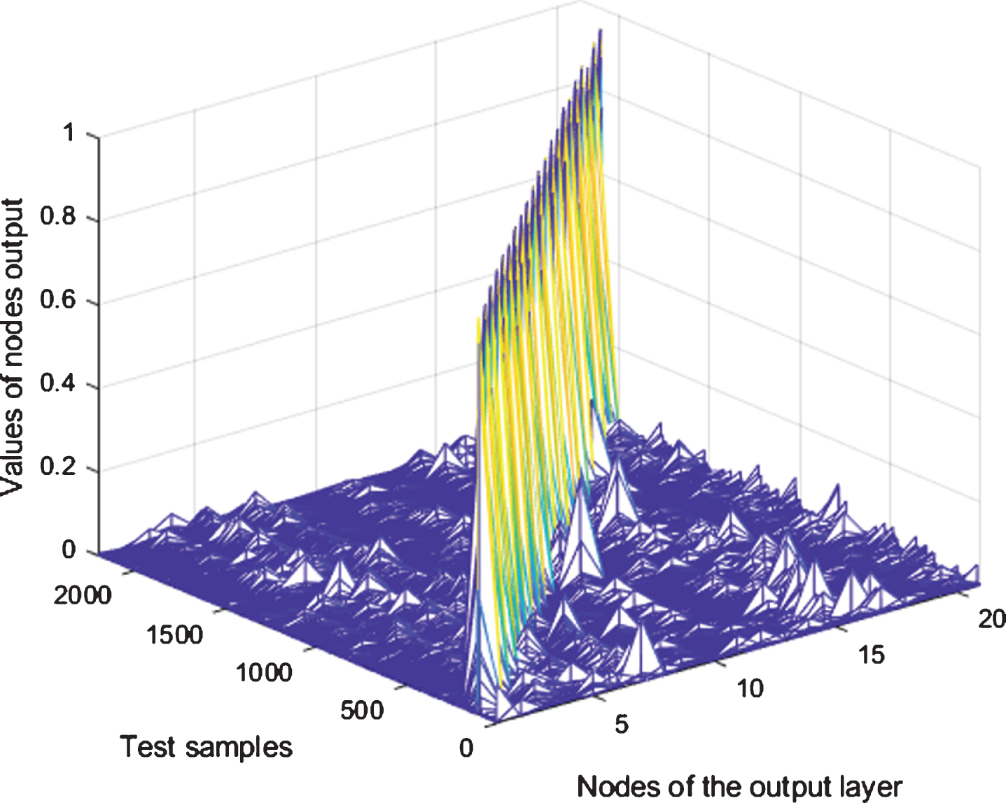
The DFFNN output corresponding to each test sample.

After processing the output of the DFFNN with a threshold of 0.7, the results are shown in Fig. 4. From this figure, we can see that the DFFNN has generalization ability in the range where there are few shifts around the training samples. For different training samples, the numbers of test samples identified by the DFFNN are not exactly the same. We then find that the DFFNN has generalization ability only within a small neighborhood around the training samples. We also learn that the DFFNN’s generalization ability is not as powerful as imagined. However, this figure does not show the category dominance phenomenon and the cross-generalization phenomenon that existed in Fig. 2.

Fig. 4

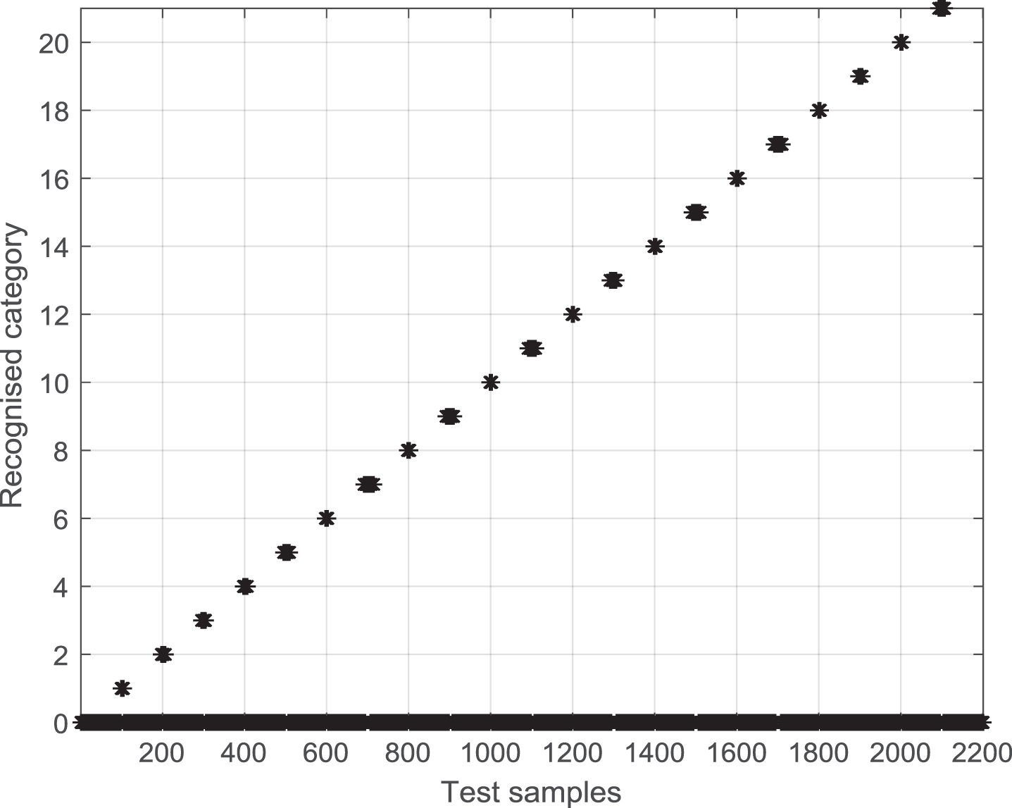
Two-dimensional view of Fig. 3 with a threshold of 0.7.

We change the structure of the DFFNN to observe the cross-class recognition phenomenon. The results are shown in Table 1. This table shows that the cross-class recognition phenomenon exists in the other two structures of the DFFNN output. Taking the DFFNN with structure 1024-380-180-80-30-21 as an example, the test results are shown in Figs. 5 6 when the batchsize is set as 1. It is clear from these two figures that the category dominance phenomenon and the cross-generalization phenomenon are very conspicuous. Hence, we learn that the quality of the network structure has a certain impact on the generalization ability of a DFFNN.

Table 1

DFFNN structures for different fault characteristics

DFFNN	Batchsize	cross-generalization
1024-260-130-80-50-21	1	None
	3	None
1024-410-260-130-80-21	1	Exist
	3	None
1024-380-180-80-30-21	1	Exist
	3	None

Fig. 5

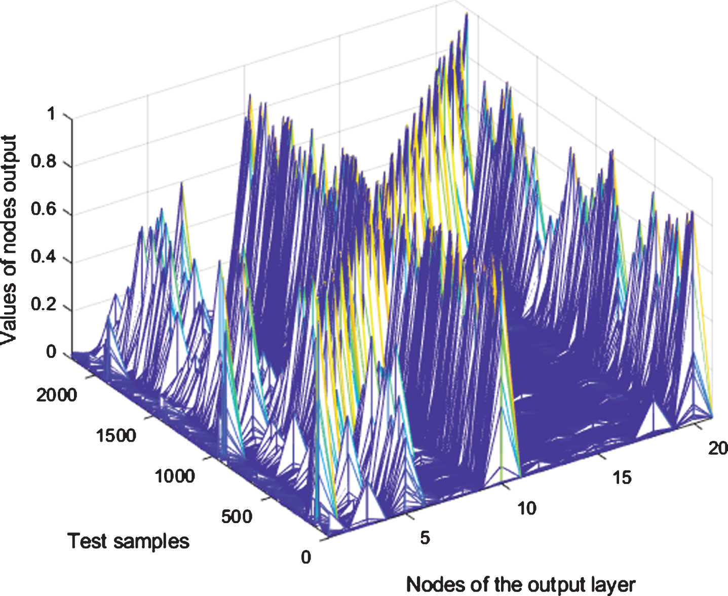
The output of the DFFNN with structure 1024-380-180-80-30-21 corresponding to each test sample.

Fig. 6

Two-dimensional view of Fig. 5 with a threshold of 0.7.

There are many factors related to the DFFNN’s generalization ability. Here, we focus on analyzing the relationship between sample similarity and the DFFNN’s generalization performance. We believe that the similarity between samples has a certain relationship with the DFFNN’s generalization performance. To confirm our hypothesis, we compare the DFFNN output and correlation coefficient of the samples.

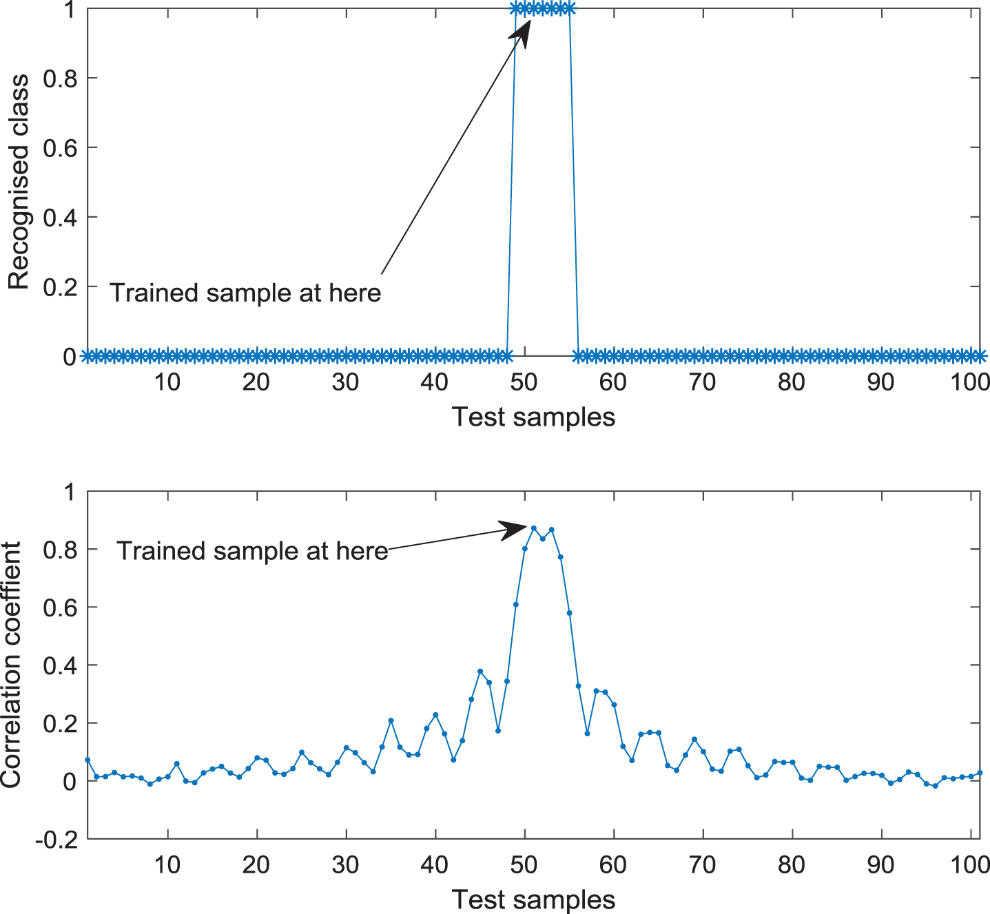
The correlation coefficient is a statistical indicator that reflects the correlation between signals. For two signals X and Y, the correlation coefficient can be calculated by [19] $r (Y, X) = \frac{Cov (X, Y)}{\sqrt{Var [X] Var [Y]}}$ (4) where Var [·] denotes the variance and Cov (·) represents the covariance. |r (Y, X) | takes a value between 0 and 1. A greater value of |r (Y, X) | indicates a greater the correlation between X and Y. Generally, the degree of correlation can be divided into strong correlation, moderate correlation, and weak correlation when |r (Y, X) | belongs to [0.6, 1], [0.4 0.6] and other values rrespectively.

The results of Fig. 3 and Fig. 4 are used for analysis purposes. Category 1 is analyzed in detail. A section of test signals whose frequencies are changed from 950 Hz to 1050 Hz are selected for the analysis. The result is shown in Fig. 7. This figure shows that the test signals can be identified as belonging to the same class as that the training sample by the DFFNN when the test sample has a strong correlation with the training samples. In contrast rthe test samples cannot be recognized as belonging to the same class as that of the training sample when the test sample has a weak correlation with the training samples. We then find that the correlation between samples can reflect the DFFNN’s generalization performance to a certain extent.

Fig. 7

An example of the DFFNN output and the correlation coefficient between samples. The top subfigure shows the DFFNN’s output for category 1 (shown in Figures 4). The bottom subfigure shows the correlation coefficient between samples.

For the results shown in Figs. 3 4 rcategory 11 is another example to be analyzed in detail. A section of test signals whose frequency is changed from 1950 Hz to 2050 Hz is selected for analysis. The result is shown in Fig. 8. This figure clearly shows the relationship between the correlation coefficient and generalization recognition. The test samples are identified as belonging to category 11 when the sample correlation is high rand they are identified as belonging to category 0 when the sample correlation is low. In particular rFig. 8 has a transition zone. The generalization result of the DFFNN fluctuates between categories 11 and 0 when the correlation coefficient transitions from strong to weak. Thus rit can be said that the similarity between samples has a certain positive correlation with the DFFNN’s generalization performance.

Fig. 8

Another example of the DFFNN output and the correlation coefficient between samples. The meaning of each subfigure is the same as that in Fig.7.

4 Improvement of the DFFNN’S generalization ability

The previous analysis showed that the DFFNN can generalize and identify test samples in a small neighborhood around the trained samples. We speculate that the DFFNN’s generalization ability can be improved by adding some similar samples to the training set. If samples are added properly rthe sum of the generalized regions of multiple samples should form a larger generalized region than before because each sample has a small generalized neighborhood. In this way rthe area of generalized recognition is expanded. Along this line of thought rwe provide a method to improve the DFFNN’s generalization ability.

The key to our method is how it obtains additional training samples with as little cost as possible. The number of samples is determined once the data collection process is complete. More data can be obtained by repeating the experiment rbut this also costs time rmanpower rmaterial resources retc. Here rwe provide a simple solution. We add some shadow samples based on the training samples to the training set. They are called shadow samples because they are very similar to the original training samples rwith only the frequency shift or amplitude changed. For example rthe model for shadow samples is written as

$\tilde{x} (i) = \tilde{Ax} (i \pm k)$ (4) where $\tilde{A}$ denotes amplitude scaling factor and k denotes the frequency shift. Amplitude and frequency are two important parameters for describing a signal. The amplitude spectrum is mainly used to display these two signal parameters. Hence rshadow samples can be easily obtained from the amplitude spectrum.

These can cause subtle differences in signal components due to load changes and speed fluctuations during industrial production. This means that shadows of training samples exist in practice. Our method takes advantage of this feature rthat is rsubtle fluctuations in signal components. The proposed method is simple and easy to implement. Some tests are presented to verify its practicality in the following subsections.

4.1 Test on simulated signals

A test is conducted to compare the results of the proposed method with the results shown in the previous section. Eight shadow samples are added for each sample rand these are ${\tilde{x}}_{1, 2} (i) = x (i \pm 2),$ (5) ${\tilde{x}}_{3, 4} (i) = \sqrt{x (i \pm 3)} .$ (6) ${\tilde{x}}_{5, 6} (i) = x (i \pm 4),$ (7) ${\tilde{x}}_{7, 8} (i) = \sqrt{x (i \pm 6)} .$ (8)

The signals shown in (5) and (7) only adjust the frequency of the training sample. The signals shown in (6) and (8) adjust the frequency of the training samples and scale their amplitudes.

A DFFNN with the same structure as before is trained on the new training set. Then rthe successfully trained DFFNN is tested by the same test set used in the previous section. The test results are shown in Fig. 9 and Fig. 10. Comparing Fig. 9 and Fig. 3 rwe can see that the DFFNN outputs of our method are more concentrated in the field of training samples. The comparison results of Fig. 10 and Fig. 4 show that the DFFNN can recognize more test samples around the trained samples by using our method than by using the existing method.

Fig. 9

The neural network output obtained by using our method that corresponds to each test sample.

Fig. 10

Two-dimensional view of Fig. 9 with a threshold of 0.7.

For a numerical comparison rdetailed identification results are shown in Table 2. It can be seen from this table that the DFFNN trained by our method can identify more test samples than that trained using the existing method. Taking the class 10 as an example rthe original DFFNN can recognize 6 test samples rbut the DFFNN trained by our method can recognize 42 test samples. The number of test samples recognize has been greatly increased. We then initially conclude that our method can improve the DFFNN’s generalization ability.

Table 2

Comparison of generalized recognition results

Class	Original method	Our method	Class	Original method	Our method
1	7	32	12	6	31
2	8	41	13	13	33
3	8	33	14	7	34
4	8	43	15	15	29
5	12	46	16	7	45
6	7	38	17	17	27
7	16	51	18	6	36
8	7	41	19	6	24
9	14	37	20	6	34
10	6	42	21	12	36
11	13	38

4.2 Test on real-world signals

We use bearing data to test the performance of our method. These data include the Case Western Reserve University (CWRU) bearing dataset 21], Paderborn University (PU) bearing dataset [22], Mechanical Failures Prevention Group (MFPT) fault dataset [23], FTP bearing dataset [24], Ottawa University (OU) bearing dataset [25], and Xi’an Jiaotong University (XJTU-SY) bearing dataset [26].

For each record, we choose a segment as a training sample and select 10 segments as test samples. Due to fluctuations in speed, changes in load, and environmental disturbances, even with the same record, there are differences in the spectrum components at different times. That is the training samples and the test samples are not exactly the same. Therefore, they can be used to test the generalization ability of DFFNNs.

The structure of the DFFNN is still set as 1024-260-130-80-50 followed by an output layer determined by the types of sample labels. For each training sample, eight shadow samples calculated by equations (8) are added. The test result is shown in Table 3. This table shows that the generalized recognition rate of our method is higher than that of the original DFFNN. Especially for MFPT, the generalized recognition rate has been increased by 23.48%which is the largest change. Table 3 shows that the generalized recognition accuracy of the DFFNN trained by our method is above 90%for these six different datasets, and two of them are 100%. Hence, it can be said that our method is effective.

Table 3
Comparison results on real-world signals

Dataset Number of training samples/class Number of test samples Original method Our method

CWRU 64/16 640 98.75 99.53

PU 152/4 1520 80.07 93.62

MFPT 23/5 230 76.52 100

FTP 119/3 1190 91.34 95.13

OU 36/3 360 96.83 98.06

XJTU-SY 466/5 4660 99.91 100

Dataset	Number of training samples/class	Number of test samples	Original method	Our method
CWRU	64/16	640	98.75	99.53
PU	152/4	1520	80.07	93.62
MFPT	23/5	230	76.52	100
FTP	119/3	1190	91.34	95.13
OU	36/3	360	96.83	98.06
XJTU-SY	466/5	4660	99.91	100

In Table 3, a training sample and test samples with the same label come from the same record. That is, the training sample and the test are homologous, and the correlation between samples is high. To further analyze the generalization ability of our method, we select training samples and test samples from different records.

The CWRU bearing data are first used for a comparative analysis. This dataset includes signals collected under different loads and speeds but with the same degree of failure [21]. One of the characteristics of CWRU bearing data is that some records are mixed with other faults, not just a single given fault [27]. This increases the difficulty of generalized recognition.

We choose the training samples and test samples from different record files. The details of the sample sets and the test results are shown in Table 4. Taking the 12k drive end bearing data as an example, the training sample includes bearing data with a load of 3 hp and a speed of 1730 rpm. The test samples are bearing data with load/speed values of 0 hp/1797 rpm, 1 hp/1772 rpm, and 2 hp/1750 rpm. We select 10 pieces of data from each record file for testing. In this way, 48 recording files form a total of 480 test samples. The generalized recognition accuracy of the original method is 60%, while the accuracy of our method is 94.17%. As a result, we obtain a high generalized recognition accuracy rate when one working condition signal is used as the training sample and the other three working condition signals are used as test samples.

Table 4

Comparison results on the CWRU bearing dataset

Position	Training samples		Test samples		Original method (%)	Our (%)	Difference (%)
	Motor load(hp)/ Shaft speed(rpm)	Number of samples/class	Motor load(hp)/ Shaft speed(rpm)	Number of samples/class
12k drive end	3/1730	15Fault+1Normal/16	0/1797 1/1772 2/1750	450Fault+30Normal/16	60	94.79	34.79
	0/1797 3/1730	30Fault+2Normal/16	1/1772 2/1750	300Fault+20Normal/16	87.81	100	12.19
12k fan end	3/1730	10Fault+1Normal/11	0/1797 1/1772 2/1750	290Fault+30Normal/11	57.19	83.75	26.56
	0/1797 3/1730	20Fault+2Normal/11	1/1772 2/1750	19Fault+2Nomal/11	63.81	90.48	26.67
48k drive end	3/1730	10Fault+1Normal/11	0/1797 1/1772 2/1750	300Fault+30Nomal/11	66.67	87.58	20.91
	0/1797 3/1730	20Fault+2Normal/11	1/1772 2/1750	200Fault+20Normal/11	84.55	99.09	14.54

Overall, Table 4 shows that the generalized recognition accuracy of our method is higher than that of the original method. The highest recognition rate achieved by our method is 100%, and that of the original method is only 87.81%. The recognition accuracy is improved by a minimum of 12.19%using our method, with a maximum of 34.79%. We learn from this that our method can indeed improve the DFFNN’s generalization ability.

The PU bearing data are then used for an additional comparative analysis. This set is a combination of data collected from healthy bearings, as well as from artificially damaged and naturally damaged bearings [22]. The damage includes inner ring (IR) damage, outer ring (OR) damage and inner ring damage mixed with outer ring (IR+OR) damage. The data were collected when the test rig was operated under different operating conditions. The main operation parameters are the rotational speed of the drive system, the radial force on the test bearing and the load torque in the drive train.

The data measured under certain conditions are used to build a training set, and the other data are used to build a test set. In the training set, one segment is taken from each data record as a training sample. In the test set, ten segments are taken from each data record as test samples. The details of the dataset and the test results are shown in Table 5.

The data with real damage are used in tests No.1 and No.3, and the data with artificial damage are used in test No.2. In contrast, the data with mixed artificial damage and real damage are used in test No. 4. Tests No. 1 and No. 2 include the IR and OR damage data. Correspondingly, tests No. 3 and No. 4 include the IR, OR, and IR+OR damage data.

Table 5

Comparison results on the PU bearing dataset

No.	Train samples		Test samples		Original method (%)	Our method (%)	Difference (%)
	Rotationalspeed(rpm)/Load Torque(Nm)/Radial force(N)	Number of samples/class	Rotationalspeed(rpm)/Load Torque(Nm)/Radial force(N)	Number of samples/class
1	1500/0.7/1000	40Fault	900/0.7/1000	600Fault	88.89	98.39	9.5
		20Normal/3	1500/0.1/1000	+300Normal/3
			1500/0.7/400
2	1500/0.7/1000	40Fault	900/0.7/1000	600Fault	78.72	88.67	9.95
		+20Normal/3	1500/0.1/1000	+300Normal/3
			1500/0.7/400
3	1500/0.7/1000	60Fault	900/0.7/1000	900Fault	80.83	92.25	11.42
		20Normal/4	1500/0.1/1000	+300Normal/4
			1500/0.7/400
4	1500/0.7/1000	60Fault	900/0.7/1000	900Fault	77.21	90	12.79
		+20Normal/4	1500/0.1/1000	+300Normal/4
			1500/0.7/400

From the comparison results shown in Table 5, we can see that our method improves the generalized recognition accuracy over that of the original method. The recognition accuracy is improved by a minimum of 9.5%and a maximum of 12.79%. Nevertheless, the increase in accuracy is slightly smaller than that for the data shown in Table 4. This also shows that our method can indeed improve the DFFNN’s generalization ability, although it achieves different performances for different datasets.

5 Conclusion

We analyzed the generalization ability of deep feedforward neural networks (DFFNNs). Tests on frequency domain signals showed that the DFFNN’s generalization ability is limited, and the DFFNN has generalization ability only within a small neighborhood around the trained samples. This leads us to believe that DFFNN’s powerful pattern recognition ability is supported by the memorization a massive amount of samples. Further analysis yields the result that the correlation coefficient between samples has a certain positive correlation with the DFFNN’s generalization performance. In real applications, some measures need to be taken to improve the DFFNN’s generalization ability.

Based on this new understanding, we proposed a method to improve DFFNN’s generalization ability. This method only uses the shadows of the trained samples instead of changing the structures of DFFNNs or training skills. Tests on some simulated signals and real-world data showed that the proposed method can indeed improve the generalization ability of a DFFNN in a very simple way. Although the test results showed that the proposed method is effective, additional tests on other datasets are needed to improve it.

Footnotes

Acknowledgments

This work was supported in part by the Natural Science Foundation of Tianjin, China under Grant 19JCYBJC16400.

References

Wang

X.Z.

, Xing

H.J.

, Li

, Hua

, Dong

C.R.

and Pedrycz

, A study on relationship between generalization abilities and fuzziness of base classifiers in ensemble learning, IEEE Transactions on Fuzzy Systems 23 (2015), 1638–1654.

Jakubovitz

, Giryes

and Rodrigues

M.R.D.

, Rodrigues, Generalization error in deep learning, arXiv,1808.01174v3, 2019.

Adam

S.P.

, Likas

A.C.

and Vrahatis

M.N.

, Evaluating generalization through interval-based neural network inversion, , Neural Computing and Applications 31 (2019), 9241–9260.

Kawaguchi

K.J.

, Kaelbling

L.P.

and Bengio

Y.S.

, Generalization in deep learning, arXiv,1710.05468v3, 2018.

Novak

, Bahri

, Abolafia

D.A.

, Pennington

and Sohl-Dickstein

, Sensitivity and generalization in neural networks: An empirical study, In: International Conference on Learning Representations, 2018. https://openreview.net/forum?id=HJC2SzZCW.

Talman

and Chatzikyriakidis

, Testing the generalization power of neural network models across NLI benchmarks, arXiv,1810.09774v2, 2018.

Neyshabur

, Bhojanapalli

, McAllester

and Srebro

, Exploring generalization in deep learning, In: 31st Conference on Neural Information Processing Systems (NIPS 2017), Long Beach, CA, USA, 2017.

Farnia

, Zhang

J.M.

and Tse

D.N.

, A Fourier-based approach to generalization and optimization in deep learning, , IEEE Journal on Selected Areas in Information Theory 1 (2020), 145–156.

Wen

, Wang

Y.D.

, Yan

, Xu

, Wu

C.P.

, Chen

Y.R.

and Li

, SmoothOut: Smoothing out sharp minima to improve generalization in deep learning, arXiv,1805.07898v3, 2018.

10.

Z.Q.J.

, Understanding training and generalization in deep learning by Fourier analysis, arXiv,1808.04295v4, 2018.

11.

Jin

P.Z.

, Lu

, Tang

Y.F.

and Karniadakis

G.E.

, Quantifying the generalization error in deep learning in terms of data distribution and neural network smoothness, , Neural Networks 130 (2020), 85–99.

12.

Schmidhuber

, Deep learning in neural networks: An overview, , Neural Networks 61 (2015), 85–117.

13.

Yang

Y.L.

and He

Y.C.

, Aweight initialization method associated with samples for deep feedforward neural network, In: International Conference on Artificial Intelligence in Electronics Engineering, Sanya, China, 2020.

14.

Hinton

G.E.

, Salakhutdinov

R.R.

and Reducing the dimensionality of data with , Neural Networks Science 313 (2006), 504–507.

15.

W.N.

, Wang

X.Q.

, Yang

C.C.

and Zhang

, A novel feature extraction method using deep neural network for rolling bearing fault diagnosis, In: 27th Chinese Control and Decision Conference (CCDC), 2427–2431, 2015.

16.

Z.Q.J.

, Zhang

Y.Y.

, Luo

, Xiao

Y.Y.

and Ma

, Frequency principle: Fourier analysis sheds light on deep Neural Networks, arXiv,1901.06523v5, 2019.

17.

Yang

Y.L.

, Fu

P.Y.

and He

Y.C.

, Bearing faults automatic classification based on deep learning, , IEEE Access 6 (2018), 71540–71554.

18.

DeepLearnToolbox website https://github.com/rasmusbergpalm/DeepLearnToolbox.

19.

Rodgers

J.L.

and Nicewander

W.A.

, Thirteen ways to look at the correlation coefficient, , The American Statistician 42 (2018), 59–66.

20.

Taylor

, Interpretation of the correlation coefficient: a basic review, , Journal of Diagnostic Medical Sonography 6 (1990), 35–39.

21.

CaseWestern Reserve University Bearing Data Center Website http://csegroups.case.edu/bearingdatacenter/home.

22.

Paderborn University Bearing Data Center Website. https://mb.uni-paderborn.de/kat/forschung/datacenter/bearing-datacenter/data-sets-and-download.

23.

Mechanical Failures Prevention Group (MFPT) Society Website. https://mfpt.org/fault-data-sets/.

24.

The Politecnico di Torino rolling bearing test rig. ftp://ftp.polito.it/people/DIRG_BearingData/.

25.

Huang

and Baddour

, Bearing vibration data collected under time-varying rotational speed conditions, Data in Brief 21 (2018), 1745–1749. https://data.mendeley.com/datasets/v43hmbwxpm/1.

26.

Wang

, Lei

Y.G.

, Li

N.P.

and Li

N.B.

, Ahybrid prognostics approach for estimating remaining useful life of rolling element bearings, IEEE Transactions on Reliability 69 (2020), 401–412. https://biaowang.tech/xjtu-sy-bearing-datasets/

27.

Smith