Introduction of a new dataset and method for location predicting based on deep learning in wargame

Abstract

It is a challenge for existing artificial intelligence algorithms to deal with incomplete information of computer tactical wargames in military research, and one effective method is to take advantage of game replays based on data mining or supervised learning. However, the open source datasets of wargame replays are extremely rare, which obstruct the development of research on computer wargames. In this paper, a data set of wargame replays is opened for predicting algorithm on the condition of incomplete information, to be specific, we propose the dataset processing method for deep learning and an network model for enemy locations predicting. We first introduce the criteria and methods of data preprocessing, parsing and feature extraction, then the training set and test set for deep learning are predefined. Furthermore, we have designed a newly specific network model for enemy locations predicting, including multi-head input, multi-head output, CNN and GRU layers to deal with the multi-agent and long-term memory problems. The experimental results demonstrate that our method achieves good performance of 84.9% on top-50 accuracy. Finally, we open source the data set and methods on https://github.com/daman043/AAGWS-Wargame-master.

Keywords

Incomplete information dataset tactical wargame locations prediction deep learning prediction model

1 Introduction

The recent significant successes in machine game such as Atari [1], the game of Go [2], and three-dimensional virtual environments [3] can be attributed to the resurgence of deep learning [4], which utilizes neural networks to provide powerful functionality for non-linear function approximation. Currently, there is a focus on a challenging domain of real-time strategy such as StarCraft II [34] [5 –7] which has issues of multi-agent, vast space, incomplete information and long-term dependence, and aims at the goal of general artificial intelligence. Meanwhile, by means of mimicking computer game technology, military researchers aim the research object at computer wargame technology, thereby advancing military intelligence decision-making capabilities.

Wargame is a general term for simulating the military operations of two or more adversaries using rules, data, and procedures to describe actual or presumed situations [8, 9]. It allows the players to explore the effects of their decisions and predict possible consequences of policies and procedures [10 –12]. As a typical kind of incomplete information games, the location and count of the enemy outside the scope of investigation are unknown. Thus computer wargame has become a challenging platform to research the military intelligent decision-making [13, 14] in recent years.

Over the past decades, there are some progress concerning the intelligent decision-making of wargame based on game theory [15], Bayesian network [16], hierarchical task planning [17, 18], data mining [19], etc. However, they lack the ability to explore large spaces and extract multi-dimensional features. Besides, the performance is not outstanding in complex scenes. As the deep learning methods make a significant breakthrough in image classification through the usage of high-level features of the target from the sample data, the DNNs (Deep Neural Networks) are widely used in machine game and achieve superhuman performance in the game of Atari games [1], Go [2] and so on. At present, research on a computer game with incomplete information is just in its infancy, and mature methods of winning have not been found. Dong et al. [20] compared the main differences and difficulties between the computer game with incomplete information and that with complete information, then the primary method of adding advantages from incomplete information is given. Moravcík M, et al. [21] trains the Deep Counterfactual Value Networks by generating random poker situations to evaluate the states of incomplete information and achieve expert-level performance. Kahng, et al. [22] propose a convolutional encoder-decoder architecture which is trained using actual game replay data. This architecture can be able to predict potential counts and locations of the opponent units based only on partially visible and noisy information. To solve the disadvantage of long-term dependence, encoder-decoder neural networks that combine convolutional neural networks with recurrent networks are proposed by Gabriel, et al. [23], and well-performing models have been trained on a large dataset of human games of StarCraft.

Above all, deepstack [21] only evaluate the states of incomplete information and give out counterfactual value for lookahead tree searching which can not applied in wargame environment. AE(Auto-Encode) networks [22, 23] give out potential counts and locations of the opponent units in form of determined value, not the probability value, that will bring out large deviation for reasoning based on knowledge. In a wargame, we need a prediction model that give out the probability of invisible opponent location. Human players rely on memory and reasoning to predict the possible locations of the enemy. Hence the computer can use machine learning technology to learn from replays to predict the distribution of enemy locations. As the wargame is an unpopular subject, relevant open source datasets and articles are extremely scarce [24, 25].

To relieve the challenge of incomplete information in wargame, we focus on the processing and methods of dataset from manual replays. Utilizing the labeled dataset of wargame, we can execute many tasks such as action prediction, state evaluation, uncertainty modeling, and inverse reinforcement learning. As an example of this dataset’s application, a DNN model based on supervised learning is proposed to solve the problem of incomplete information in wargame. In this way, we can better analyze and reason the situation information and make more intelligent decision-makings. Our main contributions are as the three following points:

We build and open source a new dataset of a tactical wargame for deep learning algorithms, which contains standard preprocessing, parsing and feature extraction procedure. The dataset is divided into the training set and test set for the convenience of evaluation and comparison with different methods.

We discuss the extraction of feature engineering in the tactical wargame and classify the features into two categories: one-dimensional features that contain attribute information and two-dimensional features that contain spatial information. Besides, the effects of different features on deep learning performance are discussed.

A new network structure called CNN-GRU for enemy locations prediction is discussed and proposed, as the baseline model we also build the ResNet network used by AlphaZero [26, 27] for comparison. We also compare the impacts of different input features on the prediction accuracy.

The rest of the paper is organized as follows. The section 2 introduces related work, which mainly includes the concept of tactical-level wargame system and enemy locations prediction. The modules of network structure employed in this paper are also introduced. In Section 3, the data processing of raw data is described, including raw data introduction, data preprocessing, parsing and feature extraction. We analyze the types of features and introduce the structures of ResNet and GRU networks in Section 4. The Section 5 describes the experimental parameters and analyzes the effects of different networks. The Section 6 briefly describes the strengths and weaknesses of our work and discusses the future research.

2 Related work

2.1 Tactical wargame profile

Traditional wargames are similar to chess games such as chess and Go in which the components are: chessboard (combat environment), chess pieces (combat entities) and referee rules (combat rules) [28]. The computer wargames sourcing from the computerization of the traditional wargames, can be expanded through an “operational scenario” to generate the specific combat environment, combat entities, and combat rules, so as to simulate a specific battlefield and allow the players to explore the effects of their decisions. Tactical-level wargame refers to the wargame system with the size of one battalion and below, and it can simulate the combat process of squad or platoon forces in a small area by flexibly using all kinds of terrain, landform, weapons, and other conditions [29]. With the characteristics of strict structure, simple rules and strong antagonism, Tactical-level wargame has grown up to be an entry-level choice for fans of wargames. As the platform of “Chinese College Students’ Wargame Competition 1 ” for three consecutive years, Armored Assault Group Wargame System 2 (AAGWS) is a typical tactical-level wargame with high popularity and representativeness. Figure 1 reveals a partial scenario of AAGWS, where the competition map is divided into hexagons. Digital at the top of the hexagonal grid is number, and the digital at the bottom is elevation. Hexagons with small black blocks are residential areas, and others are ordinary terrain. Black thick lines and red thick lines represent roads and highways, respectively. There are six pieces on each side for offensive and defensive battles in turns. One player can control multiple pieces in a round, and each piece can move multiple steps and shoot when the rules are satisfied. The two sides fought in attack and defense around the occupation points, and the scores of the game is built on the number of occupied points and attack results.

Fig. 1

Partial competition scenario of AAGWS.

In this paper, we collect the data of 670 games in the competition of the past years to serve as raw data for deep learning. Because of the limitation of the data format of AAGWS, the raw data cannot be directly used by the machine learning algorithm. It is a necessity to utilize data mining technology to develop a standard raw data processing process to generate the labeled data sets.

2.2 Dataset for deep learning in wargames

Built on stable and controllable environment, machine games are the perfect platform to test intelligent decision-making. DeepMind has conducted in-depth research on Atari series games [30 –32], Go [2, 33], and StarCraft II [34] [34, 35], which has achieved remarkable results. Table 1 compares the characteristics of Go, AAGWS and StarCraft II [34]. It can be observed that the complexity of these three kinds of games are gradually increasing. The similarities between Go and AAGWS are that they are both turn-based, and the board or map is divided into discrete and uniform grids. Still, AAGWS has the characteristics of multi-agent, multi-action and incomplete information, and the spatial complexity is far greater than Go.

Table 1
Characteristics comparison of Go, AAGWS and StarCraft II [34]

Confrontation Mode Pattern of Map Number of Agents Number of Actions in one Round Spatial Complexity Agent Attribute Information Symmetry Long Term Planning Effects of Terrain

Go Turn-Based Game Square grid Single agent Single action 10¹⁷⁰ Spatial attribute Perfect information 150–200 steps no

AAGWS Turn-Based Game Hexagonal grid Multi-agent Multi-action 10²³⁹ State property, Spatial attribute, etc. Incomplete information 500–700 steps yes

StarCraft II RTS(Real-Time Strategy Game) Pixel map Multi-agent Multi-action 10¹⁶⁸⁵ State property, Spatial attribute, etc. Incomplete information about 36000 steps yes

	Confrontation Mode	Pattern of Map	Number of Agents	Number of Actions in one Round	Spatial Complexity	Agent Attribute	Information Symmetry	Long Term Planning	Effects of Terrain
Go	Turn-Based Game	Square grid	Single agent	Single action	10¹⁷⁰	Spatial attribute	Perfect information	150–200 steps	no
AAGWS	Turn-Based Game	Hexagonal grid	Multi-agent	Multi-action	10²³⁹	State property, Spatial attribute, etc.	Incomplete information	500–700 steps	yes
StarCraft II	RTS(Real-Time Strategy Game)	Pixel map	Multi-agent	Multi-action	10¹⁶⁸⁵	State property, Spatial attribute, etc.	Incomplete information	about 36000 steps	yes

AlphaStar [7] rated at Grandmaster level effectively utilized the dataset of anonymized human replays by supervised learning and imitation learning. Recent experiment has shown that it’s difficult to train a deep neural network (DNN) end-to-end for playing StarCraft II [34] without learning human replays as AlphaGo Zero [33]. The AAGWS, of which the spatial complexity between Go and StarCraft II [34] urgently demand labeled dataset that consists of well-designed feature vectors, predefined actions and final result of each match.

There are scarce literatures about the datasets of AAGWS [36, 37]. Xing et al. [36] applied the classic Apriori algorithm to mine the rules of weapons usage from human replays and successfully explored the effectiveness of tanks, vehicles and infantry in different battle terrain. Pan et al. [37] proposed a pheromone-based model and relevant method for enemy’s location estimation in AAGWS, and give out the experimental results on the replays. However, these studies only focused on the knowledge mining of manual replays and can not boost research of advanced deep learning in wargame. After our investigation, there are no standard dataset for deep learning in tactical wargame.

To build the dataset for deeplearning from replays, Wu et al. [38] designed a standard procedure of building dataset in StarCraft II [34]. They first preprocess the replays to ensure their quality. They then parsed the replays using PySC2 3 . At last they samples and extracted feature vectors from the parsed replays subsequently and then divided all the replays into training, validation and test set.

2.3 Enemy locations prediction in wargames

In the process of tactical wargame, due to the influence of terrain fluctuation, landform, building, distance and so on, the opposing sides cannot see each other in most cases. For example, as shown in Figure 1, red tank 1 can see blue tank 1, while red tank 1 cannot see blue tank 2 as the residential areas obstruct the line of sight. Therefore, we must speculate the locations of invisible opponent pieces according to the known situation information such as the competition stages, the locations of our pieces and the visible pieces of the enemy, so as to deploy our pieces pointedly.

Human beings are capable of predicting the enemy locations based on game experience and logical reasoning, while the computer can utilize the machine learning technology to learn from replay data. The machine can predict the probability of the invisible enemy pieces locations according to the situation characteristics of the competition board. The probabilities of these locations will provide necessary information for reasoning and evaluation.

Kahng, et al. [22] proposed a method based on convolutional encoder-decoders to predict the opponent’s hidden unit information covered by the fog-of-war nature in StarCraft. To solve the disadvantage of long-term dependence, encoder-decoder neural networks that combine convolutional neural networks with recurrent networks are proposed by Gabriel, et al. [23], and the experiment shown that rule-based bot applying the networks achieved improvements in win rates. However, encoder-decoder neural networks give out potential counts and locations of the opponent units in form of determined value, not the probability value, that will bring out large deviation for reasoning based on knowledge. In wargame we only need to predict the possible location distribution of the opponents on the map.

Formally, we formulate the full state or observation in wargame as ${\bar{S}}_{t} = (B_{t}, X_{t}, {\bar{Y}}_{t})$ at time t, B_t is the global information such as map data, score, and so on, X_t is our pieces information which is the consist of individual piece state X_i,t, ${\bar{Y}}_{t}$ is enemy pieces information which is the consist of individual piece state ${\bar{Y}}_{i, t}$ . In the competition scene, one player only get partial observation which is formulated as S_t = (B_t, X_t, Y_t), Y_t is enemy pieces information which is observed by our pieces, $Y_{t} \subseteq {\bar{Y}}_{t}$ . The enemy locations prediction O_i,t is statistical variables under the condition of a sequence of past and current partial observations S₀, . . . , S_t. The prediction function can be written as: $\begin{matrix} P_{i} (O_{i, t} | S) & = P_{i} (O_{i, t} | S_{0}, . . ., S_{t}) \\ = P_{i} (O_{i, t} | (B_{0}, X_{0}, Y_{0}), . . ., (B_{t}, X_{t}, Y_{t})) \end{matrix}$ (1) where i is the index of enemy unseen piece, i ∈ [1, N], N is total number of opposite piece.

It is assumed that only the most recent L steps of a sequence partial observation contribute to the prediction of the targets, and the condition sequences can be written as S = [S_t-L+1, S_t-L+2, . . . , S_t]. Then the prediction function can be written as: $\begin{matrix} P_{i} (O_{i, t} | S) & = P_{i} (O_{i, t} | S_{t - L + 1}, . . ., S_{t}) \\ = P_{i} (O_{i, t} | (B_{t - L + 1}, X_{t - L + 1}, Y_{t - L + 1}), . . ., \\ (B_{t}, X_{t}, Y_{t})) \end{matrix}$ (2)

Both O_i,t and S are high dimensional spatial variables, one possible way is to approximate the prediction function with a parameterized depth network P_θ,i (O_i,t|S). The prediction network is trained on randomly sampled sequence pairs $[(S_{t - L + 1}, {\bar{O}}_{i, t - L + 1}), . . ., (S_{t}, {\bar{O}}_{i, t})]$ , ${\bar{O}}_{i, t}$ is the true position of piece i at time t.

The network parameters can be get by using stochastic gradient ascent to maximize the likelihood of true position $Δ θ \propto \frac{\partial log P_{θ, i} (O_{i, t} | S)}{\partial θ}$ (3)

Because of their excellent ability of spatial feature representation, CNN [39] and ResNet [27] have been successfully implemented in AlphaGo and AlphaGo Zero, respectively. Action prediction of Go is basically a classification problem with the size equaling to the size of the board. However, the enemy locations prediction of AAGWS is a classification problem whose size equals the size of wargame board. AAGWS is an incomplete information game in which the enemy pieces cannot be observed all the time. In other words, one enemy piece can be seen in one moment and be invisible in the next moment because of the movement of our piece or enemy piece. To remember the previous board information, using a memory network is a good alternative.

3 Dataset

The replay data of AAGWS consists of seven tables that record the game information, including the initial state of the pieces, the end state of the pieces, the final situation of occupation points, the action recording and the judgment information. The data composition and introduction are described in the open source project 4 . We try to build a standard dataset for DNNs according to the replay data in AAGWS, with the hope that it could serve as the benchmark for evaluating assorted algorithms in enemy locations prediction. To build our dataset, we design a standard procedure for processing the replays, as shown in Figure 2. Firstly, we preprocess the replays to ensure their quality. Then we parse the replays using the domain knowledge of AAGWS. We extract feature vectors and feature tensors from the parsed replays subsequently and finally divide all the replays into the training set and test set.

Fig. 2

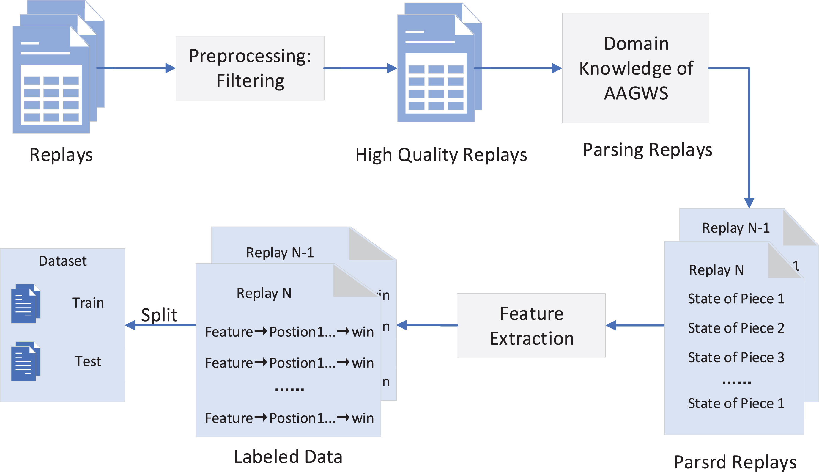
Framework overview of extracting dataset.

3.1 Preprocessing

We have collected 670 replays, which contain about 169125 action records under the “urban residential area” scenario in AAGWS. To ensure the quality of the replays in our dataset, we remain the replays which satisfy the following three criteria:

The competition time of one game must satisfy the criterion: there are 20 stages in each game, and the actual competition stage must not be less than 10.

The number of actions of each player in the initial stage should meet the following condition: the total number of actions of all pieces in the initial stage is at least 15.

The score of each player needs to satisfy the criterion: the total score of death pieces of each player can not be less than 10.

The first criterion is to remove the replays of the invalid game due to software failure or human reason. The second criterion is to dismiss the replays producing by the novice who does not know how to operate the pieces. The third criterion is to get rid of the replays in which no pieces died, which means there was no confrontation in the game. After preprocessing, we finally get 515 replays containing about 12438 action records.

3.2 Parsing replays

The replays mainly record the actions and their influences in the process of the game, which cannot directly represent the state of the board. Therefore, it is necessary to parse the replays so as to convert the events to the state of the board. Specifically, when the status of pieces changes, it is saved to form state sequence of the board, and we will get a series of states when reaching the end of a replay. Every state after parsing contains the following five parts: (1) the stage, (2) the state of occupation points, (3) the state of 12 pieces, (4) enemy locations in the previous stage, (5) competition score.

The preprocessed replays are parsed using Algorithm 1 with the domain knowledge of AAGWS. The objective is to convert the action record into the state record. Firstly, the single game replay after preprocessing recording all the actions of red and blue players is read as "one_game_actions". Then we initial the game state which will be changed after the action. We iterate the "one_game_actions" and get each action. According the effect of the action, we update the board state and save its copy and action. Finally, the states set of all the preprocessed replays can be got.

Algorithm 1 Replay Parser

Input:

DataFrame one _ game _ actions = pandas.read_csv(‘actionrecord.csv’)

Output: states

list states = []

dict state = {}

for player _ color in [red, blue] do

init state

for stage, one _ stage _ actions in one _ game _ actions do

find enemy location and update state

for action in one _ stage _ actions do

states.append((deepcopy(state), action))

switch (action):

case on_car: update state

case off_car: update state

case shoot: update state

case occupy: update state

case hide: update state

case march: update state

case cancel_keep: update state

case move: update state

end switch

end for

3.3 Extracting features

The parsed states record the complete information observed from a God-like perspective, but the players can only get the incomplete information. It is significant to extract the features of observation, enemy locations, and results to make up the labeled data pair (observation, locations, result). Feature engineering is a complex work, which needs to be determined manually under the guidance of domain knowledge. Moreover, the extracted features are not standardized and mainly be dependent on human logic analysis. According to the traits of AAGWS, the extracted features can be divided into two categories: attribute vectors and spatial tensors. To distinguish tensor from the vector, the tensor in this paper refers to the tensor with dimension > = 2.

The attribute vectors are encoded by one hot and contain 301 bits in total which consists of a few subvectors described here in order:

The stage: 20 bits.

The state of occupation points: 4 bits.

The attributes of our pieces: 23 bits for each piece, 138 bits for all 6 pieces.

The attributes of enemy pieces: 23 bits for each piece, 138 bits for all 6 pieces.

Action: 10 bit. (labeled data for supervised learning)

Result: 1 bit. (labeled data for supervised learning)

The spatial tensors mainly represent the location and visibility of the pieces. Except the elevation of the map is coded by normalization [0,1], other elements are coded by 0 and 1. It is shaped as 25×66×51 which consists of a few vectors described here in order:

The color of the player: red is 0 and blue is 1, 1×66×51.

The location of our pieces: 6 pieces in total, 6×66×51.

The location of enemy pieces under our observation: 6 pieces in total, 6×66×51.

The range of vision for enemy vehicle pieces: 1×66×51.

The range of vision for enemy soldier pieces: 1×66×51.

Tensor of the map: 4×66×51.

Enemy locations at the end of the previous stage: 6×66×51. (labeled data for supervised learning)

The above is the composition of standard features. When testing the impact of different features on prediction performance, the above features will be flexibly combined, as shown in Table 2.

Table 2
The relationship between network model and its input features

Global features The features of our pieces The features of enemy pieces Spatial rule features Map features

Color Stage Occupation points Attribute features Spatial features Attribute features Spatial features Observation range Elevation Residential Roads Normal terrain

Res-tensor ✓ ✓ ✓

Res-tensor-map ✓ ✓ ✓ ✓ ✓ ✓ ✓ ✓ ✓

Res-tensor-vector ✓ ✓ ✓ ✓ ✓ ✓ ✓ ✓ ✓ ✓ ✓ ✓

CNN-GRU ✓ ✓ ✓ ✓ ✓ ✓ ✓ ✓ ✓ ✓ ✓ ✓

		Global features	The features of our pieces	The features of enemy pieces	Spatial rule features	Map features
Res-tensor	✓				✓		✓
Res-tensor-map	✓				✓	✓	✓	✓	✓	✓	✓	✓
Res-tensor-vector	✓	✓	✓	✓	✓	✓	✓	✓	✓	✓	✓	✓
CNN-GRU	✓	✓	✓	✓	✓	✓	✓	✓	✓	✓	✓	✓

Once features are extracted, the dataset is divided into the training set and test set in the ratio 8.5:1.5, and the ratio between winners and losers preserves 1:1 in these two datasets.

3.4 Downstream tasks

Our dataset is designed for predicting enemy locations, state evaluations, and action predictions that can provide important information support for the follow-up work of intelligent decision-making. A few works that could be benefit from our dataset are list as follows:

Long Sequence Prediction. Each labeled data set is a time sequence containing observation, enemy location, action and final result. One possible task for our dataset is sequence modeling. A game dataset in AAGWS usually has 70 to 150 states, which could be used to evaluate sequence models like GRU [40], LSTM [41], NTM [42]. As for tasks in AAGWS, the dataset could be utilized for enemy locations prediction, action prediction, and global state evaluation [43, 44].

Planning and Tree Search. Games with long time steps and sparse rewards usually benefit a lot from planning and tree search algorithms. One of the most successful applications is AlphaGo, which applies the Monte Carlo tree search [45] to boost its performance. Nonetheless, the wargame cannot use the Monte Carlo tree search due to the incomplete information. Aided by a prediction model of enemy locations, a forward model of action and a global state evaluator, which are learned, it is possible to utilize planning algorithms and tree search methods.

In the next section, we focus on presenting a model and initial results for enemy locations prediction, and the rest are studied as future work.

4 Enemy locations prediction models

To build the enemy locations prediction model P_θ (O|S) (O is the location variable, S is the unperfect observation set, θ is the network parameter), we can use CNN or ResNet module for feature extracting, and use GRU module for memorizing historical information. Besides, there are two issues that need to be addressed. One is the heterogeneous feature input. AAGWS contains not only the spatial information but also the attributes of pieces, map features and so on. In general, the input features of AAGWS can be divided into two categories: one-dimensional attribute features which are represented by vectors, and two-dimensional spatial features which are represented by tensors. We transform spatial features with CNN or ResNet, and transform attribute features with full connection network, and finally use the two features in the form of data connection for subsequent processing. We also need to compare the effects of different raw features on the prediction results. The other issue is multi-task learning for multi-agent location prediction. AAGWS has six pieces per side. We need predict locations of 12 pieces considering the red and blue sides. With the share input feature extracting by neural network and the multi-head output, we use one network to realize the task of predicting the position of 12 pieces in total.

We build the prediction network called CNN-GRU that contain CNN and GRU modules and have the heterogeneous feature input and the multi-head output. To compare the different input features and network structure, we design three other models as baselines which are called Res-tensor, Res-tensor-map, and Res-tensor-vector.

4.1 Feature engineering

From the board of AAGWS, we can obtain 5 types of features: (1) The features of the global attributes, mainly including the stage, the state of the occupation points, the score, etc. (2) The features of our pieces, including the attribute features and spatial features. (3) The features of visible enemy pieces, including the attribute features and spatial features. (4) Spatial rule features, including moving range, observation range, and shooting range. (5) Map features, including elevation, landforms, buildings and so on. To compare the impact of different models and input features on the prediction results, we build 4 types of network models in 2 categories, which are named as Res-tensor, Res-tensor-map, Res-tensor-vector, CNN-GRU. Res-tensor, Res-tensor-map, and Res-tensor-vector are based on ResNet modules and they have different input features, and CNN-GRU is based on CNN and GRU modules. Table 2 shows the specific features utilized by different models. √ indicates that such features are used. The features in table 2 are obtained from dataset described in sector 3 and map data.

4.2 The prediction model based on ResNet

The ResNet is utilized to predict the action of pieces by the AlphaZero algorithm [26] which has been successfully applied to chess and shogi (Japanese chess) as well as Go. In this paper, the ResNet module is used as the basic unit to build the prediction model. According to different input features, there are three kinds of networks: Res-tensor, Res-tensor-map and Res-tensor-vector.

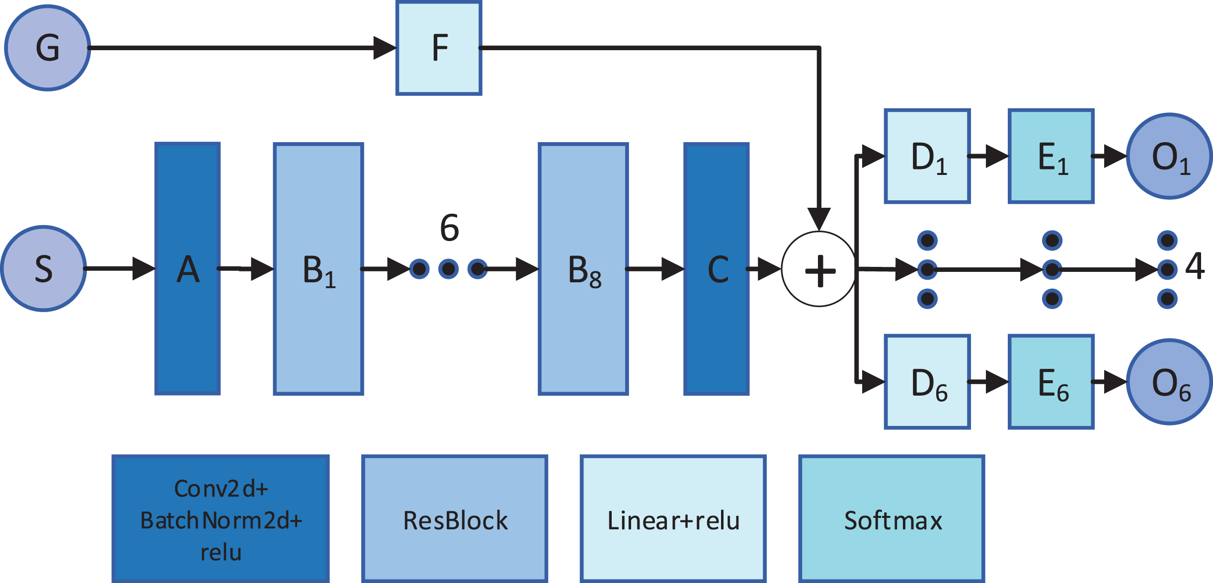
The structures of Res-tensor and Res-tensor-map are the same, except that their input features are diverse. The map features are added to the inputs of the Res-tensor-map. Figure 3 illustrates the two network structures. S is the input spatial tensor feature. A and C are composed by Conv2d, BatchNorm 2d and relu, and the kernel number of A is 20 with kernel _ size = 3, stride = 1, padding = 1, and kernel number of C is 6 with kernel _ size = 1, stride = 1, padding = 0. B₁ to B₈ are 8 ResBlocks which has 20 kernels with kernel _ size = 3, stride = 1, padding = 1. After C, the network is divided into 6 heads with the same architecture, each of which predicts the location of one piece. D₁ is a fully connected layer with the shape from 20196 to 3366. The Softmax layer E₁ output O₁ that is the prediction location distribution of piece 1. The other 5 sub-paths with the same structure output the predict location distributions of piece 2 to 6. Cross Entropy Loss serves as an objective function, which is defined as below: $J (S, \tilde{p}) = \frac{1}{M} \sum_{j = 1}^{M} \sum_{i = 1}^{N} - \tilde{p} (a_{i}^{j} | S) log p_{θ} (a_{i}^{j} | S)$ (4) where S is the input spatial tensor, $p_{θ} (a_{i}^{j} | S)$ is the probability of the j-th piece on the i-th grid predicted by the neural network with parameter θ, $\tilde{p} (a_{i}^{j} | S)$ is the true probability of the j-th piece on the i-th grid, M = 6 is the total number of pieces, N = 3366 is the total number of hexagonal grids.

Fig. 3

The structures of Res-tensor and Res-tensor-map.

The network structure of the Res-tensor-vector is similar to Res-tensor. Whereas, due to the addition of attribute vector features, the input of Res-tensor-vector is the double head. Figure 4 reveals the two network structures, where S is the input spatial tensor feature and G is the input attribute vector feature. A and C are composed by Conv2d, BatchNorm 2d and relu, and the kernel number of A is 20 with kernel _ size = 3, stride = 1, padding = 1, and the kernel number of C is 6 with kernel _ size = 1, stride = 1, padding = 0. B₁ to B₈ are 8 ResBlocks which has 20 kernels each with kernel _ size = 3, stride = 1, padding = 1. F is a fully connected layer with the shape from 288 to 100. After catenating the transmissions of spatial features and attribute features, the network is divided into 6 heads with the same architecture, and each of which predicts the location of one piece. D₁ is a fully connected layer with the shape from 20296 to 3366. Softmax layer E₁ output O₁ which is the prediction probability distribution of piece 1. The other structures are the same as Res-tensor. Cross Entropy Loss is the objective function, which is defined as below: $J (S, G, \tilde{p}) = \frac{1}{M} \sum_{j = 1}^{M} \sum_{i = 1}^{N} - \tilde{p} (a_{i}^{j} | S, G) log p_{θ} (a_{i}^{j} | S, G)$ (5) where S is the input spatial tensor, and G is the input attribute vector. $p_{θ} (a_{i}^{j} | S, G)$ is the probability of the j-th piece on the i-th grid predicted by the neural network with parameter θ, $\tilde{p} (a_{i}^{j} | S, G)$ is the true probability of the j-th piece on the i-th grid, M = 6 is the total amount of pieces, N = 3366 is the total number of hexagonal grids.

Fig. 4

The network architecture of Res-tensor-vector.

4.3 The prediction model based on GRU

Recurrent neural networks (RNNs) [46] play a significant role in the application of memory and reasoning [47]. GRU [40] is one kind of RNNs which has memory function and has been extensively used in recent years. It demonstrates good performance in dealing with Macro-management of StarCraft II [34]. In this paper, CNN and GRU are used as the basic modules to build CNN-GRU. Because the depth of feature extracting before GRU is reduced, we use CNN instead of ResNet.

Figure 5 reveals the network structure of CNN-GRU, where S_t is the input spatial tensor feature and G_t refers to the input attribute vector feature when the time is t. A, B and C composed by Conv2d, BatchNorm 2d and relu. The kernel number of A and B is 20 with kernel _ size = 3, stride = 1, padding = 1, and the kernel number of C is 6 with kernel _ size = 3, stride = 1, padding = 1. H is a fully connected layer with the size 100. After catenating the transmissions of the spatial features and attribute features, the network is divided into 6 heads with the same architecture, each of which predicts the location of one piece. D₁ is a fully connected layer with size 100. E₁ is GRU with the size 100, F₁ is a fully connected layer with size 3366. Softmax layer G₁ output O_1,t that is the prediction probability distribution of piece 1 when the time is t. The other 5 sub-paths with the same structure output the predict location distribution of piece 2 to 5.

Fig. 5

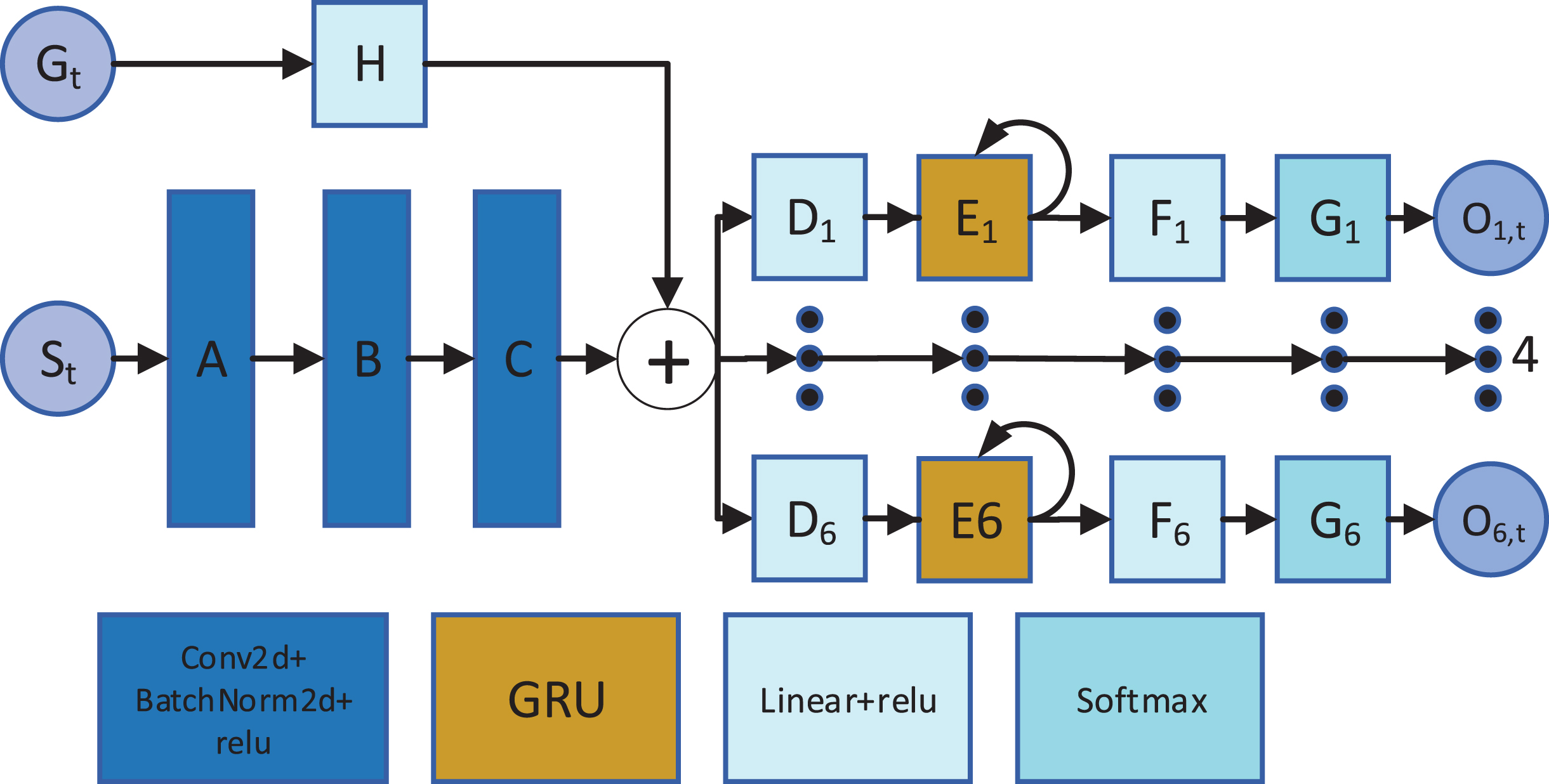
The network architecture of CNN-GRU.

The objective function is the Cross Entropy Loss, which are defined as below:

$\begin{matrix} J (S, G, \tilde{p}) & = \frac{1}{T} \frac{1}{M} \sum_{t = 1}^{T} \sum_{j = 1}^{M} \sum_{i = 1}^{N} \\ - \tilde{p} (a_{i}^{j} | S_{t}, G_{t}) log p_{θ} (a_{i}^{j} | S_{t}, G_{t}) \end{matrix}$ (6) where S stands for the set of spatial tensors in T steps which is consists of S₁, …, S_T, and G refers to the set of attribute vectors in T steps which is consists of G₁, …, G_T. $p_{θ} (a_{i}^{j} | S_{t}, G_{t})$ is the probability of the j-th piece on the i-th grid predicted by the neural network with parameter θ when the input features are S_t, G_t. $\tilde{p} (a_{i}^{j} | S_{t}, G_{t})$ is the true probability of the j-th piece on the i-th grid when the input features are S_t, G_t. M = 6 is the total number of pieces, N = 3366 is the total amount of hexagonal grids, and T = 10 is the step number of time.

5 Experimental results and analysis

5.1 Experimental environment and settings

The experimental environment is Ubuntu 18.04 with Intel Xeon E5-2620 V2 2.1GHz*24 CPU, 16G memory, 1 Tesla K40 video card. The programming language is Python, and networks are implemented using PyTorch 5 . To train the models, we use ADAM [48] for optimization. The main super parameters are provided in Table 3.

Table 3
Super parameter settings

Model name Learning rate Learning decay rate Time steps Weight decay Minibach Epoch

Res-tensor 0.001 0.7 1 0.0001 32 15

Res-tensor-map 0.001 0.7 1 0.0001 32 15

Res-tensor-vector 0.001 0.7 1 0.0001 32 15

CNN-GRU 0.0005 0.7 10 0.0001 32 15

Model name	Learning rate	Learning decay rate	Time steps	Weight decay	Minibach	Epoch
Res-tensor	0.001	0.7	1	0.0001	32	15
Res-tensor-map	0.001	0.7	1	0.0001	32	15
Res-tensor-vector	0.001	0.7	1	0.0001	32	15
CNN-GRU	0.0005	0.7	10	0.0001	32	15

In order to verify the effectiveness and practicality of the proposed model, we design a contrast experiment among the model of Res-tensor, Res-tensor-map, Res-tensor-vector and CNN-GRU. Their training set and test set are derived from the same random seed as the data processing method in Section 3. The training set of one game will be shuffled in the model of Res-tensor, Res-tensor-map and Res-tensor-vector, while the inputs of CNN-GRU are time sequence. The training results are discussed in Subsection 5.2 and test results are analyzed in Subsection 5.3. For CNN-GRU network having better performance, the influence of network depth on the performance of CNN-GRU is discussed in Subsection 5.4.

5.2 Training results

Based on the labeled data set, we train 4 network models called Res-tensor, Res-tensor-map, Res-tensor-vector, and CNN-GRU. Figure 6 illustrates a comparison of their training results, from which we can observe that the losses are convergent after 13 epochs and the accuracy reaches a higher level. Because of the muti-step input features and GRU modules, the CNN-GRU model has higher loss and a higher accuracy. We use the test data set to validation during the training process, and find all 4 model emerging distinct overfitting. In order to ensure the generalization of the model and better test results, we choose the model parameters under the best validation accuracy as the model ultimate parameters for testing.

Fig. 6

The training result. (a) The accuracy of the training. (b) The objective function loss value of the training.

5.3 Test results

5.3.1 The top-1 accuracy between different pieces

We test the models under the best-validation parameters and choose the highest accuracy as the baseline results. Figure 7 reveals the test accuracy of a single piece and the average test accuracy of all pieces. It can be observed that the test accuracy of the soldier piece is higher, because the mobility of soldier is poorer and more predictable. Overall, the performance of CNN-GRU, Res-tensor-vector, Res-tensor-map and Res-tensor decrease in turn. For models based on ResNet, the more input features are, such as adding map features (Res-tensor-map) and attribute features (Res-tensor-vector), the better performance will be achieved. Compare the two categories of models based on ResNet and GRU separately, the performance of the model based on GRU is significantly higher, which illustrates that the memory ability of GRU plays a decisive role. In summary, the CNN-GRU network with attribute vector and spatial tensor as input features achieve the best performance.

Fig. 7

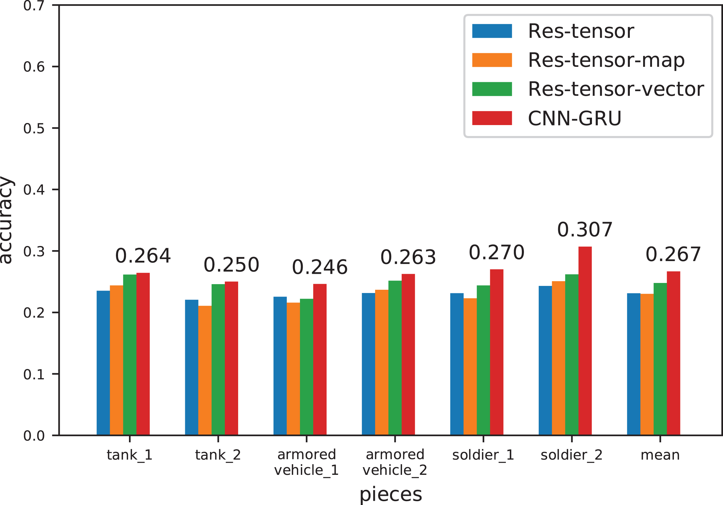
The test accuracy of a single piece and average test accuracy of all pieces.

5.3.2 The top-1 accuracy at different game stage

We test the models under best-validation parameters and study the performances at different stages. Figure 8 shows the highest accuracy rate of enemy pieces location prediction in 10 stages of red and blue each. It can be seen that the accuracy of prediction decreases with time. This reflects the regular pattern of the players moving pieces, that is, the moving path is relatively fixed at the start, but the path is more scattered and changeable at the later stage. Meanwhile, it can be observed that the prediction accuracy of CNN-GRU is absolutely highest from stage 2 to stage 6. This also reflects that the memory ability of GRU is better suited to high complexity scenarios that the pieces move more frequently and both sides see and hide continually in the middle stages.

Fig. 8

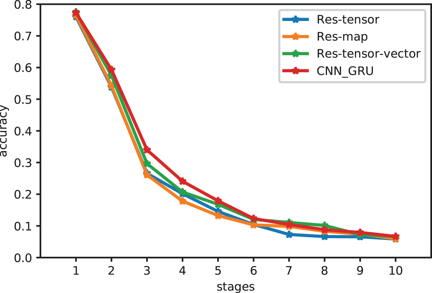
The average test accuracy in 10 stages.

5.3.3 The enemy location predicting heatmap and its real location

The output values of the models are actually the probability distributions, which reflect the possibility of pieces in a certain location on the map. Figure 9 shows a location predicting heatmap and the true locations of the tank at different time. The prediction probability of the enemy location is normalized by [0,1] as the possibility and the location where there is a green tank is the real location. With the growth of time and the expansion of the activity range of tank, the distribution of prediction probability is becoming wider (more hexagonal cells in light colors). The best prediction accuracy is at time t1, t2, t3, t4, t6, t10, and t12, and it is not accurate at time t5, t7, t8, t9 and t11. However the real locations are all on the bright hexagon, indicating that the prediction probability of the real location is not necessarily the largest, but generally larger. With the help of prediction probability, we can significantly reduce the range of possible enemy locations, and we usually use top-x accuracy, not top-one accuracy.

Fig. 9

The enemy location predicting heatmap and its true location at different time.

5.3.4 Top-x accuracy of test sets and train sets

To study the problem that the test accuracy is lower than the training accuracy, we select a portion of the training set to test the accuracy. Figure 10(a) reveals the prediction accuracy of the test set, and Figure 10(b) shows the prediction accuracy of the training set. It can be observed that the accuracy on the test set is much lower. The primary reason is the lack of training data. Even so, this network still has engineering application values. For familiar and unfamiliar opponents, the top-10 prediction accuracy rate is 81.4% and up to 57.9% respectively, which will provide vital support for intelligent decision-making.

Fig. 10

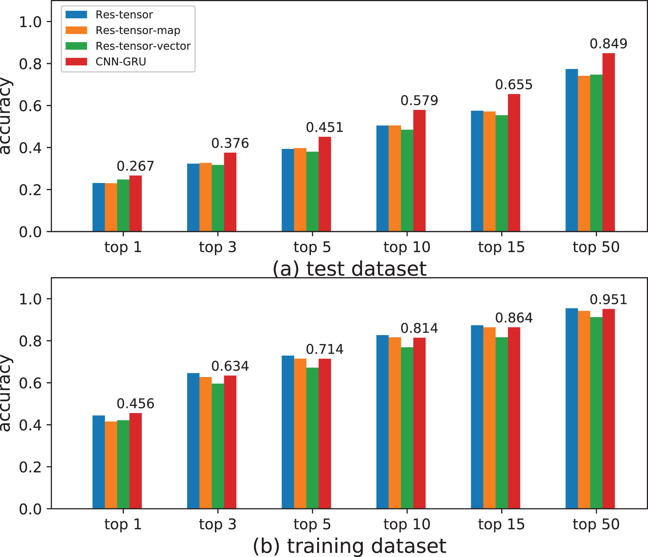
Top-x accuracy of test dataset and training dataset. (a) Test dataset prediction accuracy. (b) Training dataset prediction accuracy.

5.4 Network depth influence

To explore the influence of model depth on test performance for CNN-GRU networks, several contrast experiments are implemented as shown in Table 4. It illustrates that the test accuracy does not increase with network depth. The main reason may be the lack of training data. To overcome the impact of inadequate training data, machine self-competing and reinforcement learning will be used to generate raw data in the next phase of work.

Table 4
Test accuracy of CNN-GRU with different network depths

Network depth CNN: 3 GRU: 1 CNN: 5 GRU: 1 CNN: 5 GRU: 2 CNN: 7 GRU: 1 CNN: 7 GRU: 2 CNN: 9 GRU: 1 CNN: 9 GRU: 2

Accuracy rate 0.267 0.265 0.271 0.264 0.265 0.270 0.263

Network depth	CNN: 3 GRU: 1	CNN: 5 GRU: 1	CNN: 5 GRU: 2	CNN: 7 GRU: 1	CNN: 7 GRU: 2	CNN: 9 GRU: 1	CNN: 9 GRU: 2
Accuracy rate	0.267	0.265	0.271	0.264	0.265	0.270	0.263

6 Conclusions

In this paper, we build and open source a new dataset of a tactical wargame for deep learning algorithms, which will promote the development of computer wargame research and even promote the development of unmanned military technology. In detail, we propose a data processing method of the raw data in AAGWS, including preprocessing, parsing and feature extraction. To verify the usage of the opened dataset, 4 kinds of networks are designed to predict the enemy locations probability. The experimental results prove that the CNN-GRU network which takes attribute vector and spatial tensor as input features has the best performance, and the average of the top-10 accuracy is 57.9% on test set. However, due to the lack of raw data, the test accuracy is relatively small.

There are three main tasks for the future: firstly, we will explore a better network model, such as the network with attention mechanism to achieve state of art predicting result; secondly, we will build a network model to predict the actions of pieces and global evaluation for deep reinforcement learning; finally, we will explore an effective reasoning algorithm and design an intelligent AI for AAWGS.

Footnotes

Acknowledgments

This research was funded by the National Natural Science Foundation of China under Grant 61806221. The authors are grateful to Institute of Automation, Chinese Academy of Sciences for supplying raw replays.

References

Mnih

, Kavukcuoglu

, Silver

, Rusu

A.A.

, Veness

, Bellemare

M.G.

, Graves

, Riedmiller

, Fidjeland

A.K.

, Ostrovski

, et al., Human-level control through deep reinforcement learning, Nature 518(7540) (2015), 529.

Silver

, Huang

, Maddison

C.J.

, Guez

, Sifre

, Van Den Driessche

, Schrittwieser

, Antonoglou

, Panneershelvam

, Lanctot

, et al Mastering the game of go with deep neural networks and tree search, Nature 529(7587) (2016), 484.

Beattie

, Leibo

J.Z.

, Teplyashin

, Ward

, Wainwright

, Küttler

, Lefrancq

, Green

, Valdés

, Sadik

, et al., Deepmind lab, arXiv preprint 521(7553) (2015), 436.

LeCun

, Bengio

and Hinton

, Deep learning, Nature 521(7553) (2015), 436.

Shao

, Zhu

and Zhao

, Starcraft micromanagement with reinforcement learning and curriculum transfer learning, IEEE Transactions on Emerging Topics in Computational Intelligence 3(1) (2018), 73–84.

Peng

, Wen

, Yang

, Yuan

, Tang

, Long

and Wang

, Multiagent bidirectionally-coordinated nets: Emergence of human-level coordination in learning to play starcraft combat games, arXiv preprint arXiv:1703.10069, (2017).

Vinyals

, Babuschkin

, Czarnecki

W.M.

, Mathieu

, Dudzik

, Chung

, Choi

D. H.

, Powell

, Ewalds

, Georgiev

, et al Grandmaster level in starcraft ii using multi-agent reinforcement learning, Nature 575(7782) (2019), 350–354.

Dunnigan

J.F.

, The complete wargames handbook: How to play, design, and find them, William Morrow & Co., Inc., (1992).

Bolling

R.H.

, The joint theater level simulation in military operations other thanwar, in Proceedings of the 27th conference on Winter simulation. IEEE Computer Society (1995), 1134–1138.

10.

Davis

P.K.

, Applying artificial intelligence techniques to strategic-level gaming and simulation, Rand Corp Santa Monica Ca, Tech. Rep., (1988).

11.

Perla

P.P.

, The art of wargaming: A guide for professionals and hobbyists, Naval Institute Press, (1990).

12.

Paikowsky

and Tzezana

, The politics of space mining – an account of a simulation game, Acta Astronautica 142 (2018), 10–17. [Online]. Available: https://www-sciencedirect-com.web.bisu.edu.cn/science/article/pii/S0094576516311584.

13.

Bowling

, Fürnkranz

, Graepel

and Musick

, Machine learning and games, Machine Learning 63(3) (2006), 211–215.

14.

Langreck

, Wong

, Hernandez

A.S.

, Upton

S.C.

, Mcdonald

M.L.

, Pollman

and Hatch

W.D.

, Modeling and simulation of future capabilities with an automated computer-aided wargame:, The Journal of Defense Modeling and Simulation 154851291987398, (2019).

15.

Shubik

, The uses of teaching games in game theory classes and some experimental games, Simulation & Gaming 33(2) (2002), 139–156.

16.

Wagenhals

L.W.

and Wentz

L.K.

, New effects-based operations models in war games,” George mason univ fairfax va systems architecture lab, Tech. Rep., (2003).

17.

Hieb

, Hille

and Tecuci

, Designing a computer opponent for wargames: Integrating planning, in Knowledge Acquisition and Learning in WARGLES, AAAI Fall Symposium Series Games, (1993).

18.

Schwarz

J.O.

, Ram

and Rohrbeck

, Combining scenario planning and business wargaming to better anticipate future competitive dynamics, Futures 105 (2019), 133–142. [Online]. Available: https://www-sciencedirect-com.web.bisu.edu.cn/science/article/pii/S0016328718300545.

19.

Rushing

, Tiller

, Tanner

and McDowell

, Augmenting wargame ai with data mining technology, (2004).

20.

Dong

, Mei

, Qi

, Hou

and Li

, Research on the advantages and equilibrium of computer game with incomplete information, in 2017 29th Chinese Control And 17 Decision Conference (CCDC). IEEE, (2017), 7675–7678.

21.

Moravčík

, Schmid

, Burch

, Lisỳ

, Morrill

, Bard

, Davis

, Waugh

, Johanson

and Bowling

, Deepstack: Expert-level artificial intelligence in heads-up nolimit poker, Science 356(6337) (2017), 508–513.

22.

Kahng

, Jung

, Cho

Y.S.

, Ahn

, Park

Y.J.

, Jo

, Lee

, Do

, Lee

, Choi

, et al., Clear the fog: Combat value assessment in incomplete information games with convolutional encoder-decoders, arXiv preprint arXiv:1811.12627, (2018).

23.

Synnaeve

, Lin

, Gehring

, Gant

, Mella

, Khalidov

, Carion

and Usunier

, Forward modeling for partial observation strategy games-a starcraft defogger, in Advances in Neural Information Processing Systems (2018), 10738–10748.

24.

Zheng

S.K.

, Lin

W.U.

and Xiao-Yuan

H.E.

, The feature extraction method of wargame exercises data based on deep learning, Journal of Command & Control (2016).

25.

Moy

and Shekh

, The application of alphazero to wargaming, in AI 2019: Advances in Artificial Intelligence. Springer International Publishing (2019), 3–14.

26.

Silver

, Hubert

, Schrittwieser

, Antonoglou

, Lai

, Guez

, Lanctot

, Sifre

, Kumaran

, Graepel

, et al., A general reinforcement learning algorithm that masters chess, shogi, and go through self-play, Science 362(6419) (2018), 1140–1144.

27.

, Zhang

, Ren

and Sun

, Deep residual learning for image recognition, in Proceedings of the IEEE conference on computer vision and pattern recognition (2016), 770–778.

28.

Alexander

S.M.

, Ross

D.O.

, Vinarskai

J.S.

and Farr

S.D.

, Modeling soft factors in computer-based wargames, in Enabling Technologies for Simulation Science VI 4716. International Society for Optics and Photonics (2002), 94–98.

29.

Taylor

S.J.

, Distributed simulation: state-of-the-art and potential for operational research, European Journal of Operational Research 273(1) (2019), 1–19. [Online]. Available: https://www-sciencedirect-com.web.bisu.edu.cn/science/article/pii/S0377221718303357.

30.

Mnih

, Kavukcuoglu

, Silver

, Graves

, Antonoglou

, Wierstra

and Riedmiller

, Playing atari with deep reinforcement learning, arXiv preprint arXiv:1312.5602, (2013).

31.

Hessel

, Modayil

, Van Hasselt

, Schaul

, Ostrovski

, Dabney

, Horgan

, Piot

, Azar

and Silver

, Rainbow: Combining improvements in deep reinforcement learning, in Thirty-Second AAAI Conference on Artificial Intelligence, (2018).

32.

Aytar

, Pfaff

, Budden

, Paine

, Wang

and de Freitas

, Playing hard exploration games by watching youtube, in Advances in Neural Information Processing Systems (2018), 2930–2941.

33.

Silver

, Schrittwieser

, Simonyan

, Antonoglou

, Huang

, Guez

, Hubert

, Baker

, Lai

, Bolton

, et al., Mastering the game of go without human knowledge, Nature 550(7676) (2017), 354.

34.

Vinyals

, Ewalds

, Bartunov

, Georgiev

, Vezhnevets

A.S.

, Yeo

, Makhzani

, Küttler

, Agapiou

, Schrittwieser

, et al., Starcraft II: A new challenge for reinforcement learning, arXiv preprint arXiv:1708.04782, (2017).

35.

Zambaldi

, Raposo

, Santoro

, Bapst

, Li

, Babuschkin

, Tuyls

, Reichert

, Lillicrap

, Lockhart

, et al., Relational deep reinforcement learning, arXiv reprint arXiv:1806.01830, (2018).

36.

Xing

, Ni

, Zhang

and Yan

, Mining of weapon utility based on the replay data of war-game, Journal of Command and Control 2 (2020), 132–140.

37.

Pan

, Ni

and Yang

, An algorithm to estimate enemy’s location in wargame based on pheromone, in 2018 33rd Youth Academic Annual Conference of Chinese Association of Automation (YAC), (2018).

38.

, Zhang

and Huang

, Msc: A dataset for macromanagement in starcraft II, arXiv preprint arXiv:1710.03131, (2017).

39.

LeCun

, Boser

, Denker

J.S.

, Henderson

, Howard

R.E.

, Hubbard

and Jackel

L.D.

, Backpropagation applied to handwritten zip code recognition, Neural Computation 1(4) (1989), 541–551.

40.

Cho

, Van Merriënboer

, Bahdanau

and Bengio

, On the properties of neural machine translation: Encoder-decoder approaches, arXiv preprint arXiv:1409.1259 (2014).

41.

Hochreiter

and Schmidhuber

, Long short-term memory, Neural Computation 9(8) (1997), 1735–1780.

42.

Graves

, Wayne

and Danihelka

, Neural turing machines, arXiv preprint arXiv:1410.5401, (2014).

43.

Justesen

and Risi

, Learning macromanagement in starcraft from replays using deep learning, in 2017 IEEE Conference on Computational Intelligence and Games (CIG). IEEE, (2017), 162–169.

44.

Erickson

G.K.S.

and Buro

, Global state evaluation in starcraft, in Tenth Artificial Intelligence and Interactive Digital Entertainment Conference (2014).

45.

Coulom

, Efficient selectivity and backup operators in monte-carlo tree search, in International conference on computers and games. Springer, (2006), 72–83.

46.

Mikolov

, Karafiát

, Burget

, Černockỳ

and Khudanpur

, Recurrent neural network based language model, in Eleventh annual conference of the international speech communication association, (2010).

47.

, Chockalingam

, Singh

and Lee

, Control of memory, active perception, and action in minecraft, arXiv preprint arXiv:1605.09128, (2016).

48.

Kingma

D.P.

and Ba

, Adam: A method for stochastic optimization, arXiv preprint arXiv:1412.6980, (2014).

Introduction of a new dataset and method for location predicting based on deep learning in wargame

Abstract

Keywords

1 Introduction

2 Related work

2.1 Tactical wargame profile

3.2 Parsing replays

3.3 Extracting features

4 Enemy locations prediction models

4.1 Feature engineering

4.2 The prediction model based on ResNet

5.1 Experimental environment and settings

Table 3 Super parameter settings Model name Learning rate Learning decay rate Time steps Weight decay Minibach Epoch Res-tensor 0.001 0.7 1 0.0001 32 15 Res-tensor-map 0.001 0.7 1 0.0001 32 15 Res-tensor-vector 0.001 0.7 1 0.0001 32 15 CNN-GRU 0.0005 0.7 10 0.0001 32 15

5.3.1 The top-1 accuracy between different pieces

Table 4 Test accuracy of CNN-GRU with different network depths Network depth CNN: 3 GRU: 1 CNN: 5 GRU: 1 CNN: 5 GRU: 2 CNN: 7 GRU: 1 CNN: 7 GRU: 2 CNN: 9 GRU: 1 CNN: 9 GRU: 2 Accuracy rate 0.267 0.265 0.271 0.264 0.265 0.270 0.263

Footnotes

Acknowledgments

References

Table 3
Super parameter settings

Model name Learning rate Learning decay rate Time steps Weight decay Minibach Epoch

Res-tensor 0.001 0.7 1 0.0001 32 15

Res-tensor-map 0.001 0.7 1 0.0001 32 15

Res-tensor-vector 0.001 0.7 1 0.0001 32 15

CNN-GRU 0.0005 0.7 10 0.0001 32 15

Table 4
Test accuracy of CNN-GRU with different network depths

Network depth CNN: 3 GRU: 1 CNN: 5 GRU: 1 CNN: 5 GRU: 2 CNN: 7 GRU: 1 CNN: 7 GRU: 2 CNN: 9 GRU: 1 CNN: 9 GRU: 2

Accuracy rate 0.267 0.265 0.271 0.264 0.265 0.270 0.263