Multiperiod portfolio selection models under uncertain measure and with multiple criteria

Abstract

This paper explores a multiperiod portfolio optimization problem under uncertain measure involving background risk, liquidity constraints and V-shaped transaction costs. Unlike traditional studies, we establish multiperiod mean-variance portfolio optimization models with multiple criteria in which security returns, background asset returns and turnover rates are assumed to be uncertain variables that can be estimated by experienced experts. When the returns of the securities and background assets follow normal uncertainty distributions, we use the deterministic forms of the multiperiod portfolio optimization model. The uncertain multiperiod portfolio selection models are practical but complicated. Therefore, the models are solved by employing a genetic algorithm. The uncertain multiperiod model with multiple criteria is compared with an uncertain multiperiod model without background risk and an uncertain multiperiod model without liquidity constraint respectively, we discuss how background risk and liquidity affect optimal terminal wealth. Finally, we give two numerical examples to demonstrate the effectiveness of the proposed approach and models.

Keywords

Uncertainty theory multiple criteria uncertain multiperiod mean-variance model background risk liquidity constraint

1 Introduction

Portfolio selection focuses on how investors allocate their assets among different securities while considering a tradeoff between returns and risks and is an important issue in financial markets. Markowitz [1] first proposed a quantitative model, the mean-variance model, to study a portfolio selection problem. Using the mean-variance model, investors can obtain an optimal portfolio by maximizing the expected return for a given variance or by minimizing the variance for a given return level.

In real financial markets, numerous scholars have extended the portfolio selection models with the inclusion of multiple criteria, such as transaction costs, asset liquidity and background risk. Woodside-Oriakhi et al. [2] consider the transaction costs and investment horizon in the portfolio selection problem and illustrate the characteristics of the efficient frontier with transaction costs. Kim and Na [3] consider that security returns and turnover rates are usually asymmetrically distributed and that investors need a higher premium to purchase stocks that shift the illiquidity of the portfolio in a more right-hand direction. Investors often face changes in other sources, such as labor income, real estate income, insurance and health status. These sources of risk are referred to as background risk, and the assets that are exposed to background risk are called background assets. Since the background assets are illiquid and unhedged, it is difficult for investors to control background risk by adjusting the holdings of these assets. Therefore, it is necessary for investors to focus on total risk, including financial risk and background risk. Many studies have shown that if background risk is ignored in portfolio selection models, investors will greatly underestimate the risk of portfolios [4, 5]. Some scholars have also found that background assets, such as labor income, real estate held, entrepreneurial risk, health status and age, have a great effect on portfolio selection [6 –10]. As investors may face more than one type of background risk, the return on background assets can be regarded as a variable to study. Baptista [11] considers mental accounts in the mean-variance model with background risk, and the results reveal that the effective frontier of such portfolios is significantly different from that of portfolios without background risk. Huang and Wang [12] derive the separation theorem for two funds with background risk and employ the zero β-value CAPM theory. Jiang et al. [13] study the investors’ hedging behavior under the framework of a mean-variance model with background risk. Recently, using a mean-variance model with background risk, Guo et al. [14] discussed the behavior of banking and risk-taking. Further extending the research of Jiang et al. and Guo et al., under the mean-VaR, mean-CVaR, and mean-variance frameworks, Guo et al. [15] investigate the influence of background risk on an investor’s portfolio choice. Considering background risk, they also derive and discuss the characteristics of the mean-variance, mean-VaR, and mean-CVaR boundaries and efficient frontiers. These studies have concluded that background risk has a great influence on the optimal portfolio and efficient frontier.

However, for long-time investments, investors should continuously reallocate assets to realize their investment intention during the investment period. Mossin [16] first completes the expansion from single-period portfolio selection problems to multiperiod portfolio selection problems through a dynamic programming approach. Hakansson [17] constructs and analyzes a multiperiod portfolio selection model under a mean-variance framework. Li and Ng [18] discuss the mean-variance models for multiperiod portfolio selection optimization and analyze the analytic expressions of the optimal portfolio strategy and mean-variance effective frontier. In Li and Ng’s models, only the expected return and variance of terminal wealth are considered, while to expand Li and Ng’s models, Costa and Rodrigo [19] consider the expected return and risk of each period during the whole investment horizon. The advantage of their models is that the portfolio’s return and variance of each period can be controlled. Yu et al. [20] adopt absolute deviation as a risk measurement and develop a new multiperiod portfolio optimization model. In addition, numerous scholars establish multiperiod portfolio selection models with multiple criteria, such as consumption factors, taxes, inflation, insurance and transaction costs, to make the models more applicable to the real financial market. Considering the individual life cycle as a random variable and assuming that investors have the opportunity to buy insurance, researchers have studied the issue of multiperiod optimal investment and consumption strategies [21]. Bertsimas and Pachamanova [22] present a robust multiperiod portfolio optimization model with transaction costs. Mei et al. [23] analyze the mean-variance optimal portfolio strategy of an investor facing multiple risk assets in the presence of general transaction costs. Due to the complexity of multiperiod portfolio models, Zhang and Zhang [24] propose that the genetic algorithm can be used to solve the models.

The previous studies we reviewed suppose that the returns of risky assets and background assets can be characterized as random variables. This assumption indicates that probability distribution functions are close enough to the real frequencies. However, the financial market is also affected by many subjective factors, including social, political, and investor psychology factors. In addition, there are situations in which some unexpected events (such as financial crises) occur and securities are newly listed. Therefore, the distributions estimated from historical data may not be close enough to the frequencies of future returns because in the fast-changing financial market, historical data may be lacking or invalid. Similarly, the distribution of background asset returns cannot be estimated from historical data because of the complexity of the financial environment. In fact, Östermark [25] points out that all necessary aspects of modern finance and management (such as inventory management, risk aversion, inflation, and insurance) should be considered in the portfolio selection problem because almost all of these indeterminate situations and factors affect investment decision-making. Many scholars have implemented fuzzy set theory to solve subjective indeterminacy; for example, Huang [26], Kar et al. [27] and Kar [28] discuss the fuzzy portfolio selection problem and solution methods. Liu et al. [29] address fuzzy multiperiod portfolio selection problems considering multiple criteria. Guo et al. [30] further construct a fuzzy multiperiod portfolio selection model with different investment horizons and under multiple criteria. Using the Dempster-Shafer theory and belief entropy, Xiao [31] proposed an evidential fuzzy MCDM method, providing a novel method to deal with subjective and objective weights in the process of decision making.

However, further research [32] points out that using fuzzy set theory to characterize belief degree can lead to paradoxes. Then, for modeling the estimations of humans, Liu [33] develops the uncertainty theory, which is based on four axioms and is a branch of mathematics concerned with the analysis of belief degree. When the estimated distributions are not close enough to the real frequencies, the distribution function should be a belief degree function. To explain the difference between uncertainty and randomness, Huang and Yang [34] also show an example of uncertain stock returns. They reveal that when there are few historical data available or when historical data cannot effectively reflect the future return, to deal with indeterminacy, it is more reasonable to use uncertainty theory than probability theory. With the introduction of the uncertainty theory, Huang [35] first proposes the uncertain portfolio selection theory. Subsequently, Huang proposed many uncertain portfolio selection models based on the uncertainty theory [36 –38]. In addition, uncertain portfolio selection models considering factors, such as background risk and mental accounts are constantly being researched [34 , 40]. Huang and Yang [34] explore how background risk affects individual investment decisions under the framework of uncertainty theory and give the analytic expression of mean-variance efficient frontier. Huang and Di [40] propose an uncertain mean–variance portfolio selection model with mental accounts to reflect different attitudes towards risk. The above research only considers single-period investment, which is a one-off decision that is made at the beginning of the period and holds until the end of the period. However, to make long-term investments, investors usually need to reallocate their wealth for several consecutive periods. Therefore, a natural idea is to extend the uncertain single-period models to the uncertain multiperiod models.

Currently, there are few studies that have been conducted by using multiperiod portfolio optimization models under uncertain measure because solving uncertain multiperiod models is a complex process. Li et al. [41] investigated a multiperiod uncertain portfolio selection problem considering transaction costs and bankruptcy constraints. Chen et al. [42] researched the uncertain mean-semivariance models for multiperiod portfolio selection. Zhang [43] established multiperiod uncertain mean-absolute deviation portfolio selection models with real constraints. Jin et al. [44] formulated uncertain multiperiod portfolio selection models as tri-objective optimization problems considering chance constraints.

Different from these studies on multiperiod uncertain portfolio selection models, we formulate a multiperiod uncertain mean-variance portfolio selection problem with transaction costs, background risk and liquidity constraints. Our contributions are as follows. First, we propose a multiperiod mean-variance model based on the uncertainty theory rather than the probability theory. Uncertainty theory and probability theory have different axioms, product measures, fundamentals and operational laws. Hence, the multiperiod models and the approach to solve models based on the two theories are also different. Second, we use the variance of terminal wealth as the risk measure and propose an uncertain multiperiod mean-variance model considering transaction costs, liquidity and background risk. We also give the transformation forms of the multiperiod model for the situation in which the security returns follow a normal uncertainty distribution. Because of the complexity of the multiperiod models with multiple criteria, we employ a numerical simulation and the genetic algorithm to obtain a numerical solution. Finally, a numerical experiment is given to illustrate the application of uncertain multiperiod models with background risk and liquidity. These results reveal the importance of background risk and liquidity to portfolio selection. We also analyze the impact of background risk and liquidity on terminal wealth.

The remainder of the paper is organized as follows. In Section 2, we present the expressions of security returns, variance, transaction costs, background risk and asset liquidity at different periods by analyzing their compositions and propose the uncertain multiperiod mean-variance models. In Section 3, we prove two important theorems to state the deterministic forms of the model and discuss the impact of liquidity on the optimal portfolio return. Section 4 presents the genetic algorithm. In Section 5, two numerical examples are presented to explain the application of the proposed models. Section 6 concludes the paper.

2 Uncertain multiperiod models for portfolio selection

Different investors have different preferences, resulting in investors having various investment strategies. Therefore, to help investors make diversified investment decisions, we formulate an uncertain multiperiod portfolio model with background risk, liquidity, transaction costs and investment proportion restrictions.

2.1 Representations and assumptions

Consider n risky assets in the financial market and a planning time of T periods. Assume that the returns of n risky assets are uncertain variables. The initial wealth W₁ is allocated at the beginning of the first period, and the returns obtained at the end of each period can be reallocated at the beginning of the next period. In other words, the investors can reallocate their wealth at the beginning of the following T-1 consecutive periods. To describe the model conveniently, some notations are introduced first.

ξ_ti: the return of risky asset i at period t, where it is an uncertain variable, i = 1, 2, ... , n, t = 1, 2, ... , T;

x_ti: the investment proportion of the asset return ξ_ti, i = 1, 2, ... , n, t = 1, 2, ... , T;

x_t: the portfolio at period t, x_t = (x_t1, x_t2, . . . , x_tn), t = 1, 2, ... , T;

c_ti: the unit transaction cost of ξ_ti, i = 1, 2, ... , n, t = 1, 2, ... , T;

W_t: the uncertain wealth at the beginning of period t, t = 1, 2, ... , T;

η_ti: the uncertain turnover rate of ξ_ti and used for the measurement of asset liquidity. It is an uncertain variable, i = 1, 2, ... , n, t = 1, 2, ... , T;

r_tb: the return of background assets in period t and defined as an uncertain variable, t = 1, 2, ... , T.

2.2 Multiple criteria for the uncertain multiperiod portfolio selection problem

In this subsection, we will introduce multiple criteria, including transaction costs, background risk, terminal return, risk and asset liquidity. We assume that the entire investment process is self-financing.

(1) Transaction costs

The V-shaped transaction cost C_t is defined as being proportional to the absolute differences between portfolio x_t = (x_t1, x_t2, . . . , x_tn) at period t and portfolio x_t-1 = (x_(t-1)1, x_(t-1)2, . . . , x_(t-1)n) at period t-1, which can be expressed as follows: $C_{t} = \sum_{i = 1}^{n} c_{ti} | x_{ti} - x_{(t - 1) i} |, t = 1, 2, \dots, T,$ (1) with x_0i = 0 for any i = 1, 2, ... , n.

(2) Background risk

In long-time period investments, investors usually face different background risks in each period, and we assume that the background asset returns in each period may follow different uncertainty distributions. Suppose that r_tb denotes background asset returns in period t and ξ_t1, ξ_t2, . . . , ξ_tn denotes the uncertain return rates of n risky assets in period t. Then, the return rate of the portfolio in period t can be written as follows: $R_{t} = \sum_{i = 1}^{n} (ξ_{ti} x_{ti} - c_{ti} | x_{ti} - x_{(t - 1) i} |) + r_{tb} .$ (2)

(3) Expected terminal wealth

Considering transaction costs and background risk, the terminal wealth at the end of the tth period (or at the beginning of the (t + 1)th period) is the following $\begin{matrix} W_{t + 1} = W_{t} \times [1 + \sum_{i = 1}^{n} (ξ_{ti} x_{ti} - c_{ti} | x_{ti} - x_{(t - 1) i} |) + r_{tb}], \\ t = 1, 2, \dots, T . \end{matrix}$ (3)

In general, it can be assumed that the return of the background assets is independent of the return of n risky assets. According to formulation (3), it is clear that W_T+1 is a function of ξ_t1, ξ_t2, . . . , ξ_tn and r_tb, t = 1, 2, ... , T. Since ξ_t1, ξ_t2, . . . , ξ_tn and r_tb are all uncertain variables, W_T+1 is also an uncertain variable. The expected value of uncertain terminal wealth at each period in the investment process can be expressed as follows: $E [W_{2}] = W_{1} \times E [1 + \sum_{i = 1}^{n} (ξ_{1 i} x_{1 i} - c_{1 i} | x_{1 i} - x_{0 i} |) + r_{1 b}],$ (4)

$\begin{matrix} E [W_{3}] = E [W_{2} \times (1 + \sum_{i = 1}^{n} (ξ_{2 i} \\ x_{2 i} - c_{2 i} | x_{2 i} - x_{1 i} |) + r_{2 b})], \end{matrix}$ (5) ⋮

$\begin{matrix} E [W_{T + 1}] = E [W_{T} \times (1 + \sum_{i = 1}^{n} \\ (ξ_{Ti} x_{Ti} - c_{Ti} | x_{T i} - x_{(T - 1) i} |) + r_{Tb})] . \end{matrix}$ (6)

Thus, the expected terminal wealth at the end of T can be obtained in the following:

$\begin{matrix} E [W_{T + 1}] = W_{1} \times E [\prod_{t = 1}^{T} (1 + \sum_{i = 1}^{n} \\ (ξ_{ti} x_{ti} - c_{ti} | x_{t i} - {x (t - i)}_{i} |) + r_{tb})] . \end{matrix}$ (7)

(4) Variance of terminal wealth

On the other hand, risk is measured by the variance of the uncertain terminal wealth W_t+1, and the cumulative risk over T periods can be computed by the following: $\begin{matrix} V (x) = Var (W_{T + 1}) = Var [W_{T} \times (1 + \sum_{i = 1}^{n} \\ (ξ_{Ti} x_{Ti} - c_{Ti} | x_{Ti} - x_{(T - 1) i} |) + r_{Tb})] \\ = Var [W_{1} \times \prod_{t = 1}^{T} (1 + \sum_{i = 1}^{n} \\ (ξ_{ti} x_{ti} - c_{ti} | x_{ti} - x_{(t - 1) i} |) + r_{tb})] \\ = W_{1}^{2} \times Var [\prod_{t = 1}^{T} (1 + \sum_{i = 1}^{n} \\ (ξ_{ti} x_{ti} - c_{ti} | x_{ti} - x_{(t - 1) i} |) + r_{tb})] \end{matrix}$ (8)

(5) Assets liquidity

Liquidity is defined as the chance of converting an investment into cash without any significant loss in value. Investors prefer portfolios with high liquidity when other conditions are the same. In this paper, the turnover rate is used to measure asset liquidity. Let (η_t1, η_t2, . . . , η_tn) be the uncertain turnover rate of n assets in period t. Then, the expected turnover rate $E [\sum_{i = 1}^{n} η_{ti} x_{ti}]$ represents the liquidity of the portfolio x_t = (x_t1, x_t2, …, x_tn) in period t. The cumulative liquidity L(x) of n assets over T investment periods is measured by the sum of the expected turnover rate of the portfolio during each investment period. Therefore, we can calculate L(x) by the following formulation: $L (x) = \sum_{t = 1}^{T} [E [\sum_{i = 1}^{n} η_{ti} x_{ti}]] .$ (9)

2.3 Uncertain multiperiod portfolio selection models

This subsection will study the multiperiod uncertain portfolio selection problem with multiple criteria, such as returns, risk, background risk, transaction cost and asset liquidity. Rational investors hope to maximize their total return while minimizing risk. However, in the financial market, the two objectives of high return and low risk are difficult to achieve at the same time because a higher return is usually accompanied by higher risk. In addition, aggressive investors have a strong risk tolerance, and they are more concerned about the total return obtained during the investment period. In this situation, the objective function of the multiperiod uncertain portfolio selection model is to maximize expected terminal wealth at the end of period T, and the uncertain multiperiod mean-variance model can be formulated as follows: ${\begin{matrix} max E [W_{T + 1}] = W_{1} \times E [\prod_{t = 1}^{T} (1 + \sum_{i = 1}^{n} \\ (ξ_{ti} x_{ti} - c_{ti} | x_{ti} - x_{(t - 1) i} |) + r_{tb})] \\ subject to : \\ V (W_{T + 1}) = W_{1}^{2} \times Var [\prod_{t = 1}^{T} (1 + \sum_{i = 1}^{n} \\ (ξ_{ti} x_{ti} - c_{ti} | x_{ti} - x_{(t - 1) i} |) + r_{tb})] ⩽ β, \\ L (x) = \sum_{t = 1}^{T} [E [\sum_{i = 1}^{n} η_{ti} x_{ti}]] ⩾ l, \\ \sum_{i = 1}^{n} x_{ti} = 1, t = 1, 2, . . ., T, \\ W_{t + 1} = W_{t} \times [1 + \sum_{i = 1}^{n} (ξ_{ti} x_{ti} + r_{tb} - c_{ti} \\ | x_{ti} - x_{(t - 1) i} |], \\ 0 ⩽ x_{ti} ⩽ u_{ti} ⩽ 1, i = 1, 2, . . ., n; t = 1, 2, . . ., T . \end{matrix}$ (10)

In model (10), we assume W₁ = 1. The first constraint indicates that the risk of the terminal wealth of the portfolio must be less than or equal to the preset maximum risk tolerance level β. The second constraint requires that the cumulative liquidity of the risky assets should reach or exceed the minimum acceptable liquidity level l given by investors. The third constraint indicates that the sum of the investment proportions at period t must be unity. The fourth constraint is the wealth accumulation constraint, that is, the relationship between the wealth at period t + 1 and that at period t. The fifth constraint is the proportion restriction, which provides the lower and upper bounds of x_ti.

Unlike aggressive investors, conservative investors want to minimize the cumulative risk when the return of uncertain terminal wealth is greater than the expected return level. The multiperiod uncertain portfolio selection model should be as follows: ${\begin{matrix} min V (x) = W_{1}^{2} \times Var [\prod_{t = 1}^{T} (1 + \sum_{i = 1}^{n} \\ (ξ_{ti} x_{ti} - c_{ti} | x_{ti} - x_{(t - 1) i} |) + r_{tb})] \\ subject to : \\ E [W_{T + 1}] = W_{1} \times E [\prod_{t = 1}^{T} (1 + \sum_{i = 1}^{n} \\ (ξ_{ti} x_{ti} - c_{ti} | x_{ti} - x_{(t - 1) i} |) + r_{tb})] ⩾ α, \\ L (x) = \sum_{t = 1}^{T} [E [\sum_{i = 1}^{n} η_{ti} x_{ti}]] ⩾ l, \\ \sum_{i = 1}^{n} x_{ti} = 1, t = 1, 2, . . ., T, \\ W_{t + 1} = W_{t} \times [1 + \sum_{i = 1}^{n} (ξ_{ti} x_{ti} + r_{tb} - c_{ti} \\ | x_{ti} - x_{(t - 1) i} |)], \\ 0 ⩽ x_{ti} ⩽ u_{ti} ⩽ 1, i = 1, 2, . . ., n; t = 1, 2, . . ., T . \end{matrix}$ (11) where α is the given minimum return level. The first constraint ensures that the expected value of the terminal wealth in the portfolio must be greater than or equal to the preset minimum return level α accepted by investors. The remaining constraints have the same meanings as those in model (10).

Example 1. Suppose that there is a two-period uncertain portfolio selection problem with four risky assets. Let the return rates of the four assets be ξ_t1, ξ_t2, ξ_t3, ξ_t4, where t = 1, 2 and let all variables be uncertain variables. Let r_tb, t = 1, 2, be the return rate of the background assets, and let it also be an uncertain variable. The corresponding wealth at different periods can be calculated by the following formulas: $W_{1} = 1,$ $W_{2} = W_{1} \times [1 + \sum_{i = 1}^{4} (ξ_{1 i} x_{1 i} - c_{1 i} x_{1 i}) + r_{1 b}],$ $W_{3} = W_{2} \times [1 + \sum_{i = 1}^{4} (ξ_{2 i} x_{2 i} - c_{2 i} | x_{2 i} - x_{1 i} |) + r_{2 b}] .$

If the investor is aggressive, the uncertain two-period portfolio selection model can be established as follows: ${\begin{matrix} max E [W_{3}] = E [(1 + \sum_{i = 1}^{4} (ξ_{1 i} x_{1 i} - c_{1 i} x_{1 i}) + r_{1 b}) \\ (1 + \sum_{i = 1}^{4} (ξ_{2 i} x_{2 i} - c_{2 i} | x_{2 i} - x_{1 i} |) + r_{2 b})] \\ subject to : \\ Var [W_{3}] = Var [(1 + \sum_{i = 1}^{4} (ξ_{1 i} x_{1 i} - c_{1 i} x_{1 i}) + r_{1 b}) \\ (1 + \sum_{i = 1}^{4} (ξ_{2 i} x_{2 i} - c_{2 i} | x_{2 i} - x_{1 i} |) + r_{2 b})] ⩽ β, \\ \sum_{t = 1}^{2} [E [\sum_{i = 1}^{4} η_{ti} x_{ti}]] ⩾ l, \\ \sum_{i = 1}^{4} x_{ti} = 1, t = 1, 2 . \\ 0 ⩽ x_{ti} ⩽ u_{ti} ⩽ 1, i = 1, 2, 3, 4; t = 1, 2 . \end{matrix}$ (12)

Conservative investors pursue minimal risk under a given acceptable return level. The uncertain multiperiod portfolio selection model should be the following: ${\begin{matrix} max Var [W_{3}] = Var [(1 + \sum_{i = 1}^{4} (ξ_{1 i} x_{1 i} - c_{1 i} x_{1 i}) + r_{1 b}) \\ (1 + \sum_{i = 1}^{4} (ξ_{2 i} x_{2 i} - c_{2 i} | x_{2 i} - x_{1 i} |) + r_{2 b})] \\ subject to : \\ E [W_{3}] = E [(1 + \sum_{i = 1}^{4} (ξ_{1 i} x_{1 i} - c_{1 i} x_{1 i}) + r_{1 b}) \\ (1 + \sum_{i = 1}^{4} (ξ_{2 i} x_{2 i} - c_{2 i} | x_{2 i} - x_{1 i} |) + r_{2 b})] ⩾ α, \\ \sum_{t = 1}^{2} [E [\sum_{i = 1}^{4} η_{ti} x_{ti}]] ⩾ l, \\ \sum_{i = 1}^{4} x_{ti} = 1, t = 1, 2 . \\ 0 ⩽ x_{ti} ⩽ u_{ti} ⩽ 1, i = 1, 2, 3, 4; t = 1, 2 . \end{matrix}$ (13)

Furthermore, without consideration of the background risk, the terminal return of W_T+1 can be calculated as $\prod_{t = 1}^{T} (1 + \sum_{i = 1}^{n} (ξ_{ti} x_{ti} - c_{ti} | x_{ti} - x_{(t - 1) i} |))$ . Then, model (10) can be degenerated into the following form, which is the uncertain multiperiod portfolio model without background risk: ${\begin{matrix} max E [W_{T + 1}] = E [\prod_{t = 1}^{T} (1 + \sum_{i = 1}^{n} \\ (ξ_{ti} x_{ti} - c_{ti} | x_{ti} - x_{(t - 1) i} |))] \\ subject to : \\ V (W_{T + 1}) = Var [\prod_{t = 1}^{T} (1 + \sum_{i = 1}^{n} (ξ_{ti} x_{ti} - c_{ti} \\ | x_{ti} - x_{(t - 1) i} |))] ⩽ β, \\ L (x) = \sum_{t = 1}^{T} [E [\sum_{i = 1}^{n} η_{ti} x_{ti}]] ⩾ l, \\ \sum_{i = 1}^{n} x_{ti} = 1, t = 1, 2, . . ., T, \\ W_{t + 1} = W_{t} \times [1 + \sum_{i = 1}^{n} (ξ_{ti} x_{ti} - c_{ti} | x_{ti} - x_{(t - 1) i} |)], \\ 0 ⩽ x_{ti} ⩽ u_{ti} ⩽ 1, i = 1, 2, . . ., n; t = 1, 2, . . ., T . \end{matrix}$ (14)

If we do not consider asset liquidity, there is no third constraint in model (10). The multiperiod uncertain portfolio model without asset liquidity but with background risk can be expressed as follows: ${\begin{matrix} max E [W_{T + 1}] = W_{1} \times E [\prod_{t = 1}^{T} \\ (1 + \sum_{i = 1}^{n} (ξ_{ti} x_{ti} - c_{ti} | x_{ti} - x_{(t - 1) i} |) + r_{tb})] \\ subject to : \\ V (W_{T + 1}) = Var [\prod_{t = 1}^{T} (1 + \sum_{i = 1}^{n} \\ (ξ_{ti} x_{ti} - c_{ti} | x_{ti} - x_{(t - 1) i} |) + r_{tb})] ⩽ β, \\ \sum_{i = 1}^{n} x_{ti} = 1, t = 1, 2, . . ., T, \\ W_{t + 1} = W_{t} \times [1 + \sum_{i = 1}^{n} (ξ_{ti} x_{ti} + r_{tb} - c_{ti} \\ | x_{ti} - x_{(t - 1) i} |)], \\ 0 ⩽ x_{ti} ⩽ u_{ti} ⩽ 1, i = 1, 2, . . ., n; t = 1, 2, . . ., T . \end{matrix}$ (15)

A comparison of model (15) with model (10) reveals that model (15) has the same objective function as model (10). Additionally, the optimal solution of model (10) is a feasible solution of model (15), but the optimal solution of model (15) is not necessarily a feasible solution of model (10). Therefore, the optimal solution of model (10) is not greater than that of model (15); that is, the expected terminal wealth of the optimal multiperiod portfolio considering asset liquidity is not greater than that of the optimal multiperiod portfolio without asset liquidity.

Similar to the previous literature [4 , 13], we assume that the return rate of the background assets at period t follows the normal uncertainty distribution and that r_tb ∼ N (e_tb, ρ_tb), t = 1, 2, ... , T. Next, some deterministic forms of multiperiod uncertain models are derived.

3 Deterministic equivalents of the uncertain models

Since the multiperiod uncertain model (10) is complex and contains the expected value and variance of uncertain variables, it cannot be solved directly. Next, to facilitate solving the model, the deterministic forms of the multiperiod uncertain model (10) will be given.

Theorem 1. Suppose that the return rates ξ_t1, ξ_t2, . . . , ξ_tn and the turnover rates η_t1, η_t2, . . . , η_tn on n risky assets at period t are uncertain variables. Let the uncertainty distribution of ξ_ti be Φ_ti (·), and the uncertainty distribution of r_tb be Θ_t (·), i = 1, 2, ... , n, t = 1, 2, ... , T. Then, the multiperiod uncertain model (10) can be converted into the following deterministic form: ${\begin{matrix} max E [W_{T + 1}] = \int_{0}^{1} Ψ^{- 1} (α) d α \\ subject to : \\ Var [W_{T + 1}] = \int_{0}^{1} (Ψ^{- 1} (α) - E [W_{T + 1}])^{2} d α ⩽ β, \\ Ψ^{- 1} (α) = \prod_{t = 1}^{T} [1 + \sum_{i = 1}^{n} (x_{ti} Φ_{ti}^{- 1} (α) - c_{ti} \\ | x_{ti} - x_{(t - 1) i} |) + Θ_{t}^{- 1} (α)] \\ \sum_{t = 1}^{T} \sum_{i = 1}^{n} E [η_{ti} x_{ti}] ⩾ l, \\ \sum_{i = 1}^{n} x_{ti} = 1, t = 1, 2, . . ., T, \\ W_{t + 1} = W_{t} \times [1 + \sum_{i = 1}^{n} (ξ_{ti} x_{ti} + r_{tb} - c_{ti} \\ | x_{ti} - x_{(t - 1) i} |)], \\ 0 ⩽ x_{ti} ⩽ u_{ti} ⩽ 1, i = 1, 2, . . ., n; t = 1, 2, . . ., T . \end{matrix}$ (16)

Proof. When the security return ξ_ti and turnover rate η_ti are all uncertain variables, the return rate of the portfolio $\sum_{i = 1}^{n} ξ_{ti} x_{ti}$ and the turnover rate of the portfolio $\sum_{i = 1}^{n} η_{ti} x_{ti}$ at period t are also the uncertain variables, i = 1, 2, ... , n, t = 1, 2, ... , T. Let Ψ denote the uncertainty distribution of terminal wealth $W_{T + 1} = W_{1} \times [\prod_{t = 1}^{T} (1 + \sum_{i = 1}^{n} (ξ_{ti} x_{ti} - c_{ti} | x_{(t + 1) i} - x_{ti} |) + r_{tb})]$ . Similar to what Li et al. [41] have studied, we can find that $M {1 + \sum_{i = 1}^{n} (ξ_{ti} x_{ti} + r_{tb} - c_{ti} | x_{ti} - x_{(t - 1) i} |) > 0} = 1$ is true when M {ξ_ti + r_tb > 2ɛ_t - 1} =1 for i = 1, 2, ... , n, t = 1, 2, ... , T, ɛ_t = max {c_t1, c_t2, . . . , c_tn}. Let Ψ denote the uncertainty distribution of $\prod_{t = 1}^{T} (1 + \sum_{i = 1}^{n} (ξ_{ti} x_{ti} - c_{ti} | x_{(t + 1) i} - x_{ti} |) + r_{tb})$ . In the following research, we assume that M {ξ_ti + r_tb > 2ɛ_t - 1} =1 for i = 1, 2, ... , n, t = 1, 2, ... , T. Therefore, we know that $1 + \sum_{i = 1}^{n} (ξ_{ti} x_{ti} + r_{tb} - c_{ti} | x_{ti} - x_{(t - 1) i} |)$ is a positive uncertain variable. Then, W_T+1 is also a positive uncertain variable and strictly increases with ξ_ti and r_tb. According to the operational law of uncertain variables, we can obtain the following inverse uncertainty distribution function of Ψ: $\begin{matrix} Ψ^{- 1} (α) = W_{1} \times \prod_{t = 1}^{T} [1 + \sum_{i = 1}^{n} (x_{ti} Φ_{ti}^{- 1} (α) - c_{ti} \\ | x_{ti} - x_{(t - 1) i} |) + Θ_{t}^{- 1} (α)] . \end{matrix}$ (17)

Then, the expected value and variance of W_T+1 are given as follows. $\begin{matrix} E [W_{T + 1}] = E [\prod_{t = 1}^{T} (1 + \sum_{i = 1}^{n} (ξ_{ti} x_{ti} - c_{ti} \\ | x_{(t + 1) i} - x_{ti} |) + r_{tb})] = \int_{0}^{1} Ψ^{- 1} (α) d α \\ = \int_{0}^{1} \prod_{t = 1}^{T} [1 + \sum_{i = 1}^{n} (x_{ti} Φ_{ti}^{- 1} (α) - c_{ti} \\ | x_{ti} - x_{(t - 1) i} |) + Θ_{t}^{- 1} (α)] d α = e, \end{matrix}$ (18) $\begin{matrix} Var [W_{T + 1}] = Var [\prod_{t = 1}^{T} (1 + \sum_{i = 1}^{n} (ξ_{ti} x_{ti} - c_{ti} \\ | x_{(t + 1) i} - x_{ti} |) + r_{tb})] = \int_{0}^{1} (Ψ^{- 1} (α) - e)^{2} d α \\ = \int_{0}^{1} [\prod_{t = 1}^{T} (1 + \sum_{i = 1}^{n} (x_{ti} Φ_{ti}^{- 1} (α) - c_{ti} | x_{ti} \\ - x_{(t - 1) i} |) + Θ_{t}^{- 1} (α)) - e]^{2} d α, \end{matrix}$ (19) $E [\sum_{t = 1}^{T} \sum_{i = 1}^{n} η_{ti} x_{ti}] = \sum_{t = 1}^{T} \sum_{i = 1}^{n} E [η_{ti}] x_{ti} .$ (20)

Substituting the above three expressions into model (10) to obtain model (16), Theorem 1 is proven.

Theorem 1 presents the deterministic form of the multiperiod mean-variance model with background risk and a liquidity constraint based on uncertainty theory in the general case. Thus, when the returns of assets, the returns of background assets, and turnover rates all follow normal uncertainty distributions, we can obtain the deterministic equivalent of model (10).

Theorem 2. Suppose that ξ_ti, η_ti and r_tb are normal uncertain variables; i.e., ξ_ti ∼ N (e_ti, σ_ti), $η_{ti} \sim N (e_{ti}^{'}, σ_{ti}^{'})$ and r_tb ∼ N (e_tb, ρ_tb), i = 1, 2, ... , n, t = 1, 2, ... , T. Then, model (14) can be transformed into the following deterministic form: ${\begin{matrix} max E [W_{T + 1}] = \int_{0}^{1} Ψ^{- 1} (α) d α \\ subject to : \\ Var [W_{T + 1}] = \int_{0}^{1} (Ψ^{- 1} (α) - E [W_{T + 1}])^{2} d α ⩽ β, \\ Ψ^{- 1} (α) = \prod_{t = 1}^{T} [1 + \sum_{i = 1}^{n} x_{ti} (e_{ti} + \frac{\sqrt{3} σ_{ti}}{π} ln \frac{α}{1 - α}) \\ - \sum_{i = 1}^{n} c_{ti} | x_{ti} - x_{(t - 1) i} | + e_{tb} + \frac{\sqrt{3} ρ_{tb}}{π} ln \frac{α}{1 - α}] \\ \sum_{t = 1}^{T} \sum_{i = 1}^{n} e_{ti}^{'} x_{ti} ⩾ l, \\ \sum_{i = 1}^{n} x_{ti} = 1, t = 1, 2, . . ., T, \\ W_{t + 1} = W_{t} \times [1 + \sum_{i = 1}^{n} (ξ_{ti} x_{ti} + r_{tb} - c_{ti} \\ | x_{ti} - x_{(t - 1) i} |)], \\ 0 ⩽ x_{ti} ⩽ u_{ti} ⩽ 1, i = 1, 2, . . ., n; t = 1, 2, . . ., T . \end{matrix}$ (21)

Proof. Since ξ_ti and r_tb are normal uncertain variables, i.e., since ξ_ti ∼ N (e_ti, σ_ti) and r_tb ∼ N (e_tb, σ_tb), i = 1, 2, ... , n, t = 1, 2, ... , T, then, the uncertainty inverse distributions of ξ_ti and r_tb can be denoted by the following: $Φ_{ti}^{- 1} (α) = e_{ti} + \frac{\sqrt{3} σ_{ti}}{π} ln \frac{α}{1 - α},$ $Θ_{t}^{- 1} (α) = e_{tb} + \frac{\sqrt{3} σ_{tb}}{π} ln \frac{α}{1 - α} .$

When η_ti is a normal uncertain variable and $η_{ti} \sim N (e_{ti}^{'}, σ_{ti}^{'})$ , $\sum_{t = 1}^{T} \sum_{i = 1}^{n} η_{ti} x_{ti}$ is also a normal uncertain variable and $\sum_{t = 1}^{T} \sum_{i = 1}^{n} η_{ti} x_{ti} \sim N (\sum_{t = 1}^{T} \sum_{i = 1}^{n} e_{ti}^{'} x_{ti}, \sum_{t = 1}^{T} \sum_{i = 1}^{n} σ_{ti}^{'} x_{ti})$ . Therefore, the expected value of cumulative liquidity is $\sum_{t = 1}^{T} \sum_{i = 1}^{n} e_{ti}^{'} x_{ti}$ .

Therefore, Theorem 2 is proved.

In addition, according to Theorem 2, let ξ_ti, η_ti and r_tb be normal uncertain variables, i.e., ξ_ti ∼ N (e_ti, σ_ti), $η_{ti} \sim N (e_{ti}^{'}, σ_{ti}^{'})$ and r_tb ∼ N (e_tb, ρ_tb), i = 1, 2, ... , n, t = 1, 2, ... , T, respectively. We can obtain the deterministic forms of the multiperiod uncertain model without background risk and without asset liquidity, ${\begin{matrix} max E [W_{T + 1}] = \int_{0}^{1} Ψ^{- 1} (α) d α \\ subject to : \\ Var [W_{T + 1}] = \int_{0}^{1} (Ψ^{- 1} (α) - E [W_{T + 1}])^{2} d α ⩽ β, \\ Ψ^{- 1} (α) = \prod_{t = 1}^{T} [1 + \sum_{i = 1}^{n} x_{ti} (e_{ti} + \frac{\sqrt{3} σ_{ti}}{π} ln \frac{α}{1 - α}) \\ - \sum_{i = 1}^{n} c_{ti} | x_{ti} - x_{(t - 1) i} |] \\ \sum_{t = 1}^{T} \sum_{i = 1}^{n} e_{ti}^{'} x_{ti} ⩾ l, \\ \sum_{i = 1}^{n} x_{ti} = 1, t = 1, 2, . . ., T, \\ W_{t + 1} = W_{t} \times [1 + \sum_{i = 1}^{n} (ξ_{ti} x_{ti} - c_{ti} | x_{ti} - x_{(t - 1) i} |)], \\ 0 ⩽ x_{ti} ⩽ u_{ti} ⩽ 1, i = 1, 2, . . ., n; t = 1, 2, . . ., T . \end{matrix}$ (22) and ${\begin{matrix} max E [W_{T + 1}] = \int_{0}^{1} Ψ^{- 1} (α) d α \\ subject to : \\ Var [W_{T + 1}] = \int_{0}^{1} (Ψ^{- 1} (α) - E [W_{T + 1}])^{2} d α ⩽ β, \\ Ψ^{- 1} (α) = \prod_{t = 1}^{T} [1 + \sum_{i = 1}^{n} x_{ti} (e_{ti} + \frac{\sqrt{3} σ_{ti}}{π} ln \frac{α}{1 - α}) \\ - \sum_{i = 1}^{n} c_{ti} | x_{ti} - x_{(t - 1) i} | + e_{tb} + \frac{\sqrt{3} ρ_{tb}}{π} ln \frac{α}{1 - α}] \\ \sum_{i = 1}^{n} x_{ti} = 1, t = 1, 2, . . ., T, \\ W_{t + 1} = W_{t} \times [1 + \sum_{i = 1}^{n} (ξ_{ti} x_{ti} + r_{tb} - c_{ti} \\ | x_{ti} - x_{(t - 1) i} |)], \\ 0 ⩽ x_{ti} ⩽ u_{ti} ⩽ 1, i = 1, 2, . . ., n; t = 1, 2, . . ., T . \end{matrix}$ (23)

4 Genetic algorithm

Since the models proposed in Section 3 are nonlinear programming problems, we cannot solve them directly by using traditional approaches; therefore, the heuristic algorithm is an alternative method to solve nonlinear models. The genetic algorithm (GA) has always been regarded as an effective and practical algorithm for solving nonlinear programming problems, and was originally proposed by Holland [45]. Currently, to solve portfolio optimization problems, it is still employed by many researchers, such as Li et al. [41] and Huang [46]. We first use a numerical method to compute the expected value and variance of the terminal return, and then we integrate the results into a genetic algorithm. Taking model (10) as an example, the steps in solving the multiperiod uncertain model can be summarized as follows.

(1) Compute the expected value and variance of uncertain terminal wealth

First, we calculate E [W_T+1] by the inverse uncertainty distribution function. We assume that the security return ξ_ti has the continuous uncertainty distribution function Φ_ti (α) and that the background asset return r_tb has the uncertainty distribution function Θ_t (α). The inverse uncertainty distribution function Ψ^-1 (α) of $\prod_{t = 1}^{T} [1 + \sum_{i = 1}^{n} (ξ_{ti} x_{ti} - c_{ti} | x_{ti} - x_{(t - 1) i} |) + r_{tb}]$ can be expressed as $Ψ^{- 1} (α) = \prod_{t = 1}^{T} [1 + \sum_{i = 1}^{n} (x_{ti} Φ_{ti}^{- 1} (α) - c_{ti} | x_{ti} - x_{(t - 1) i} |) + Θ_{t}^{- 1} (α)]$ . Then, we can calculate the expected value of W_T+1 by E [W_T+1] = $\int_{0}^{1} \prod_{t = 1}^{T} [1 + \sum_{i = 1}^{n} (x_{ti} Φ_{ti}^{- 1} (α) - c_{ti} | x_{ti} - x_{(t - 1) i} |) + Θ_{t}^{- 1} (α)] d α$ . The integral can be calculated by transforming it into the discrete form $\frac{1}{N} \sum_{k = 1}^{N} \prod_{t = 1}^{T} [1 + \sum_{i = 1}^{n} (x_{ti} Φ_{ti}^{- 1} (ς_{k}) - c_{ti} | x_{ti} - x_{(t - 1) i} |) + Θ_{t}^{- 1} (ς_{k})]$ , ς_k ∈ (0, 1).

Second, we can calculate the variance of the terminal wealth Var [W_T+1] by $Var [W_{T + 1}] = \int_{0}^{1} (Ψ^{- 1} (α) - e)^{2} d α$ and the variance can also be calculated by the discrete form.

(2) Genetic Algorithm

Variable representation. For the multiperiod uncertain portfolio selection models, the solution X = (x₁₁, x₁₂, . . . , x_1n ; . . . ; x_T1, x_T2, . . . , x_Tn) is encoded by a chromosome V = (v₁₁, v₁₂, . . . , v_1n ; . . . ; v_T1, v_T2, . . . , v_Tn) where v_ti are nonnegative numbers, t = 1, 2, ... , T, i = 1, 2, ... , n. The encoding and decoding processes are determined by the equations x_ti = v_ti/(v_t1 + v_t2 + . . . + v_tn), which ensures that x_t1 + x_t2 + . . . + x_tn = 1 always holds at all periods, t = 1, 2, ... , T.

Initialization. Given the integer pop_size, which is defined as the size of the population, randomly generate a chromosome and check the feasibility of this chromosome. Accept the chromosome as a feasible chromosome if it satisfies the corresponding constraint conditions in model (10). If not, reject the chromosome, and regenerate a chromosome until a feasible chromosome is obtained. Repeat the above operation until the pop_size feasible chromosomes V₁, V₂, ... , V_{pop_size} are obtained.

Evaluation function. The rank-based evaluation function is employed in the GA, which is used to measure the likelihood of reproduction for each chromosome. For model (10), a chromosome with a larger value of E [W_T+1] has a higher fitness value; i.e., the chromosome with a higher terminal expected return is better. Given a parameter a ∈ [0, 1], the rank-based evaluation function is defined as follows: $Eval (V_{i}) = a (1 - a)^{i - 1}, i = 1, 2, . . ., pop_size .$

Specifically, i = 1 denotes the best individual, and i = pop_size denotes the worst individual.

Selection process. The selection process is performed according to spinning the roulette wheel. First, define the cumulative probability p_k for each chromosome V_k as follows, $p_{0} = 0, p_{k} = \sum_{i = 1}^{k} Eval (V_{i}), k = 1, 2, \dots, pop_size .$

Next, generate a random number r ∈ (0, p_{pop_size}]. If p_k-1 < r ⩽ p_k, and select the kth chromosome V_k. Repeat the two steps pop_size times and pop_size chromosomes can be selected.

Crossover. Denote a parameter p_c as the probability of crossover. Generate a random number r ∈ [0, 1] and select the k chromosome V_k (k = 1, 2, ... , pop_size) if r < p_c. If the number of selected chromosomes is odd, redo the above operation until the number becomes even. Then, divide those selected chromosomes into the following pairs: (Z₁, Z₂), (Z₃, Z₄),.... Generate a random number ς ∈ (0, 1), and then conduct the crossover process: $Z_{j} = ς Z_{j} + (1 - ς) Z_{j + 1}, Z_{j + 1} = ς Z_{j + 1} + (1 - ς) Z_{j} .$

Note that the feasibility of each child must be checked; that is, redo the above procedure until two feasible children are obtained. Then, replace the parents with two chromosomes chosen from the parents and children with higher fitness values. Repeat the above process pop_size times.

Mutation. Similarly, conduct the following process from i = 1 to pop_size. Define p_m as the probability of mutation. Generate a random number; chromosome V_i is chosen if r < p_m. Let K be a sufficiently large positive number. Choose d as the direction of the mutation. If V_i + Kd is a feasible chromosome, replace V_i with V_i + Kd.

We summarize the GA as follows,

Initialize pop_size chromosomes and use the inverse uncertainty distribution function to solve the constraints.

Compute the objective values for all chromosomes.

Calculate the fitness of each chromosome by a rank-based evaluation function.

Select the chromosomes by spinning the roulette wheel.

Update the chromosomes by conducting crossover and mutation operations.

Repeat steps 2–5 for a given number of generations.

Report the best chromosome, and decode it within the solution of the portfolio selection model.

5 Numerical experiment

Two numerical examples will be provided to illustrate the effectiveness of the multiperiod uncertain models and the genetic algorithm. Suppose an investor would like to choose 6 stocks for his multiperiod investment. The two examples aim to illustrate the impact of background risk and asset liquidity on multiperiod uncertain portfolio models.

Example 1. The investor intends to construct a four-period investment strategy with initial wealth W₁ = 10000 RMB. Therefore, in the model, n = 6, and T = 4. Through a historical data analysis and expert estimation, we can obtain uncertainty distributions of return rates and turnover rates. Assume that the return rate ξ_ti of stock i at period t is an uncertain normal variable ξ_ti ∼ N (μ_ti, σ_ti) and that the turnover rate η_ti of stock i at period t is also an uncertain normal variable $η_{ti} \sim N (μ_{ti}^{'}, σ_{ti}^{'})$ . The uncertainty distributions of the return rate and turnover rate for the 6 stocks are shown in Tables 1 and 2. Suppose that the transaction costs of 6 stocks in each period are identical; i.e., c_ti = 0.003 for all i = 1, 2, …, 6, t = 1, 2, 3, 4. The return rates of the background assets r_tb in each period follow the same distribution, and we assume r_tb ∼ N (0.008.0.005) for all t = 1, 2, 3, 4. The risk level β and the minimal liquidity level l are set to 0.01 and 1, respectively. Let the upper bound of the investment proportion be 0.6.

Table 1
Uncertainty distributions of return rates for 6 stocks

Period Stock 1 Stock 2 Stock 3

1 N(0.0085, 0.01) N(0.0106, 0.024) N(0.0103, 0.015)

2 N(0.0099, 0.011) N(0.0102, 0.015) N(0.0098, 0.011)

3 N(0.0101, 0.016) N(0.0097, 0.011) N(0.0101, 0.012)

4 N(0.0100, 0.014) N(0.0105, 0.017) N(0.0102, 0.013)

Period Stock 4 Stock 5 Stock 6

1 N(0.0106, 0.019) N(0.0109, 0.01) N(0.0105, 0.014)

2 N(0.0098, 0.016) N(0.0105, 0.012) N(0.0099, 0.013)

3 N(0.01, 0.007) N(0.0102, 0.009) N(0.0099, 0.008)

4 N(0.0101, 0.011) N(0.0104, 0.008) N(0.0104, 0.018)

Period	Stock 1	Stock 2	Stock 3
1	N(0.0085, 0.01)	N(0.0106, 0.024)	N(0.0103, 0.015)
2	N(0.0099, 0.011)	N(0.0102, 0.015)	N(0.0098, 0.011)
3	N(0.0101, 0.016)	N(0.0097, 0.011)	N(0.0101, 0.012)
4	N(0.0100, 0.014)	N(0.0105, 0.017)	N(0.0102, 0.013)
Period	Stock 4	Stock 5	Stock 6
1	N(0.0106, 0.019)	N(0.0109, 0.01)	N(0.0105, 0.014)
2	N(0.0098, 0.016)	N(0.0105, 0.012)	N(0.0099, 0.013)
3	N(0.01, 0.007)	N(0.0102, 0.009)	N(0.0099, 0.008)
4	N(0.0101, 0.011)	N(0.0104, 0.008)	N(0.0104, 0.018)

Table 2

Uncertainty distributions of turnover rates for 6 stocks

Period	Stock 1	Stock 2	Stock 3	Stock 4	Stock 5	Stock 6
1	N(0.39, 0.25)	N(0.54, 0.34)	N(0.14, 0.05)	N(0.56, 0.47)	N(0.68, 0.36)	N(0.23, 0.12)
2	N(0.51, 0.30)	N(0.51, 0.42)	N(0.31, 0.13)	N(0.36, 0.18)	N(0.34, 0.20)	N(0.20, 0.09)
3	N(0.29, 0.16)	N(0.32, 0.26)	N(0.29, 0.13)	N(0.41, 0.22)	N(0.20, 0.11)	N(0.13, 0.10)
4	N(0.54, 0.42)	N(0.46, 0.52)	N(0.34, 0.24)	N(0.57, 0.44)	N(0.50, 0.46)	N(0.19, 0.20)

Table 3

The iterations and parameters of genetic algorithm

Iterations	pop_size	p _c	p _m	Generation
1000	240	0.8	0.2	500

We will numerically calculate the expected value and variance of terminal wealth and employ a genetic algorithm to solve the portfolio selection models. The iterations and parameters of the genetic algorithm are set as follows.

Case 1. Using the portfolio selection model with background risk and liquidity constraints, if the investor wants to pursue the maximum expected terminal wealth, he/she can obtain the optimal portfolios of all four periods by solving model (24). Table 4 shows the optimal portfolio in each period. We calculate that the expected terminal wealth is 10862 RMB. ${\begin{matrix} max E [W_{T + 1}] = \int_{0}^{1} Ψ^{- 1} (α) d α \\ subject to : \\ Var [W_{T + 1}] = \int_{0}^{1} (Ψ^{- 1} (α) - E [W_{T + 1}])^{2} d α ⩽ 0.01, \\ Ψ^{- 1} (α) = \prod_{t = 1}^{4} [1 + \sum_{i = 1}^{6} x_{ti} (e_{ti} + \frac{\sqrt{3} σ_{ti}}{π} ln \frac{α}{1 - α}) \\ - \sum_{i = 1}^{6} 0.003 \times | x_{ti} - x_{(t - 1) i} | + 0.008 \\ + \frac{\sqrt{3} \times 0.005}{π} ln \frac{α}{1 - α}] \\ \sum_{t = 1}^{4} \sum_{i = 1}^{6} e_{ti}^{'} x_{ti} ⩾ 1, \\ \sum_{i = 1}^{6} x_{ti} = 1, t = 1, 2, 3, 4, \\ W_{t + 1} = W_{t} \times [1 + \sum_{i = 1}^{6} (ξ_{ti} x_{ti} + r_{tb} - 0.003 \\ \times | x_{ti} - x_{(t - 1) i} |)], \\ 0 ⩽ x_{ti} ⩽ u_{ti} ⩽ 1, i = 1, 2, . . ., 6; t = 1, 2, 3, 4 . \end{matrix}$ (24)

Table 4

The optimal portfolios for the model with background risk and liquidity constraint

Period	Stock 1	Stock 2	Stock 3	Stock 4	Stock 5	Stock 6
1	0.4973	0.0000	0.0000	0.0000	0.1617	0.3409
2	0.5704	0.0000	0.3087	0.0000	0.1156	0.0053
3	0.0000	0.0837	0.0885	0.1595	0.2626	0.4056
4	0.0058	0.0000	0.2451	0.0899	0.5522	0.1070
Expected return	10862

Case 2. If we do not consider the liquidity constraint in the uncertain multiperiod portfolio selection model, we will solve model (25) to obtain the optimal portfolio. The optimal portfolios at all 4 periods are shown in Table 5, and the expected terminal wealth is 10913 RMB. It can be seen that the optimal expected wealth with background risk but without a liquidity constraint is greater than that with background risk and a liquidity constraint and that the optimal portfolios are quite different between two situations. A comparison of model (10) with model (23) reveals that this is a general conclusion. ${\begin{matrix} max E [W_{T + 1}] = \int_{0}^{1} Ψ^{- 1} (α) d α \\ subject to : \\ Var [W_{T + 1}] = \int_{0}^{1} (Ψ^{- 1} (α) - E [W_{T + 1}])^{2} d α ⩽ 0.01, \\ Ψ^{- 1} (α) = \prod_{t = 1}^{4} [1 + \sum_{i = 1}^{6} x_{ti} (e_{ti} + \frac{\sqrt{3} σ_{ti}}{π} ln \frac{α}{1 - α}) \\ - \sum_{i = 1}^{6} 0.003 \times | x_{ti} - x_{(t - 1) i} | + 0.008 \\ + \frac{\sqrt{3} \times 0.005}{π} ln \frac{α}{1 - α}] \\ \sum_{i = 1}^{6} x_{ti} = 1, t = 1, 2, 3, 4, \\ W_{t + 1} = W_{t} \times [1 + \sum_{i = 1}^{6} (ξ_{ti} x_{ti} + r_{tb} - 0.003 \\ \times | x_{ti} - x_{(t - 1) i} |)], \\ 0 ⩽ x_{ti} ⩽ u_{ti} ⩽ 1, i = 1, 2, . . ., 6; t = 1, 2, 3, 4 . \end{matrix}$ (25)

Table 5

The optimal portfolios for the model without liquidity constraint

Period	Stock 1	Stock 2	Stock 3	Stock 4	Stock 5	Stock 6
1	0.3616	0.0091	0.2700	0.0046	0.2816	0.0731
2	0.3569	0.0056	0.3349	0.0016	0.2279	0.0731
3	0.0031	0.0411	0.0030	0.5244	0.0089	0.4195
4	0.0281	0.0767	0.0086	0.4450	0.3613	0.0803
Expected return	10913

Case 3. Regarding the uncertain portfolio selection problem with a liquidity constraint but without background risk, we can obtain the optimal investment strategies by solving model (26), and the results are presented in Table 6. We obtain the optimal expected terminal wealth: 10588 RMB. We find that the optimal expected wealth solved by the uncertain multiperiod portfolio selection model with a liquidity constraint but without background risk is smaller than that with a liquidity constraint and background risk. The reason is that the return rate of the background assets is zero when we do not consider the background risk in the model; therefore, the total return also decreases.

Table 6

The optimal portfolios for the model without background risk

Period	Stock 1	Stock 2	Stock 3	Stock 4	Stock 5	Stock 6
1	0.1353	0.1784	0.2370	0.0635	0.0581	0.3277
2	0.1337	0.2345	0.2305	0.0603	0.0135	0.3275
3	0.1025	0.2586	0.0359	0.2080	0.0657	0.3275
4	0.1022	0.1659	0.1993	0.3517	0.0581	0.1228
Expected return	10588

{\begin{matrix} max E [W_{T + 1}] = \int_{0}^{1} Ψ^{- 1} (α) d α \\ subject to : \\ Var [W_{T + 1}] = \int_{0}^{1} (Ψ^{- 1} (α) - E [W_{T + 1}])^{2} d α ⩽ 0.01, \\ Ψ^{- 1} (α) = \prod_{t = 1}^{4} [1 + \sum_{i = 1}^{6} x_{ti} (e_{ti} + \frac{\sqrt{3} σ_{ti}}{π} ln \frac{α}{1 - α}) \\ - \sum_{i = 1}^{6} 0.003 \times | x_{ti} - x_{(t - 1) i} |] \\ \sum_{t = 1}^{4} \sum_{i = 1}^{6} e_{ti}^{'} x_{ti} ⩾ 1, \\ \sum_{i = 1}^{6} x_{ti} = 1, t = 1, 2, 3, 4, \\ W_{t + 1} = W_{t} \times [1 + \sum_{i = 1}^{6} (ξ_{ti} x_{ti} - 0.003 \\ \times | x_{ti} - x_{(t - 1) i} |)], \\ 0 ⩽ x_{ti} ⩽ u_{ti} ⩽ 1, i = 1, 2, . . ., 6; t = 1, 2, 3, 4 . \end{matrix}

(26)

For the optimal portfolios we computed in the three cases, Fig. 1 shows the investment proportions of 6 stocks over 4 periods. In this example, guaranteeing the diversification of the security investment, the investment proportion of each stock is less than 0.6.

Fig.1

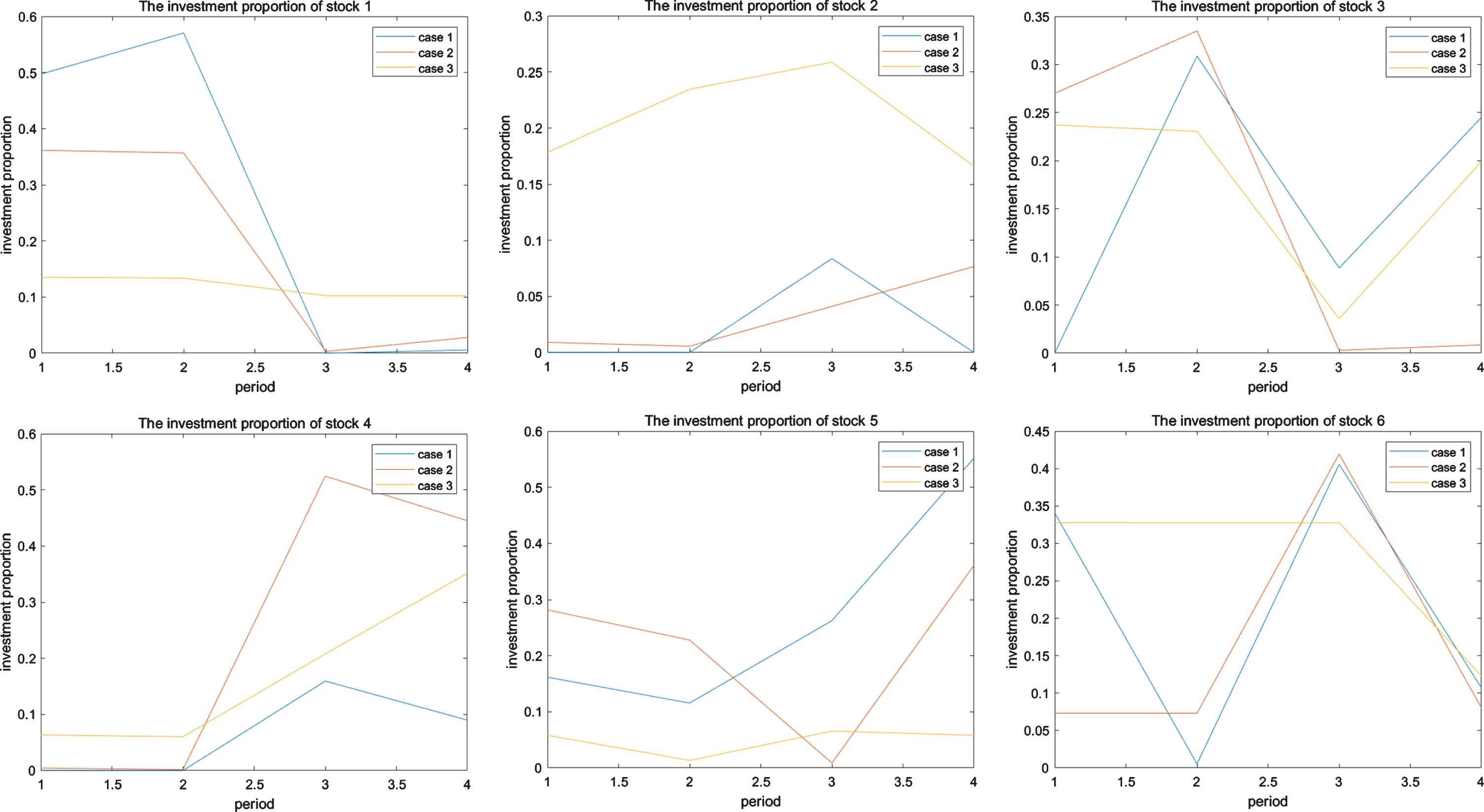
The investment proportions of 6 stocks.

Example 2. Assuming W₁ = 1, β= 0.01 and the return rate of background assets is the same for each period, we change the values of background assets return e_b and study the effect of background assets return on the optimal expected terminal wealth. The results are provided in Table 7, which shows that when e_b increases, the optimal terminal wealth increases.

Table 7

Expected terminal wealth for different expected returns of background assets

e	0	0.002	0.004	0.006	0.008	0.01	0.012
Expected terminal wealth	1.0577	1.0615	1.0697	1.0754	1.0862	1.0946	1.1005

Additionally, we assume that the risk level is 0.02 and that the return of the background assets is 0. We change the values of standard deviation ρ and study how the standard deviation of the background assets ρ affects the investment risk. The results in Table 8 reveal that as ρ increases, the investment risk increases. We can draw the same conclusion as that reached for the single-period situation; i.e., ignoring the background risk may underestimate the investment risk. These results are also visually presented in Fig. 2.

Table 8

Standard deviations of terminal wealth for different standard deviations of background assets

ρ	0	0.001	0.002	0.003	0.004	0.005	0.006
Standard deviation	0.088	0.0943	0.1022	0.1032	0.1046	0.1107	0.1179

Fig.2

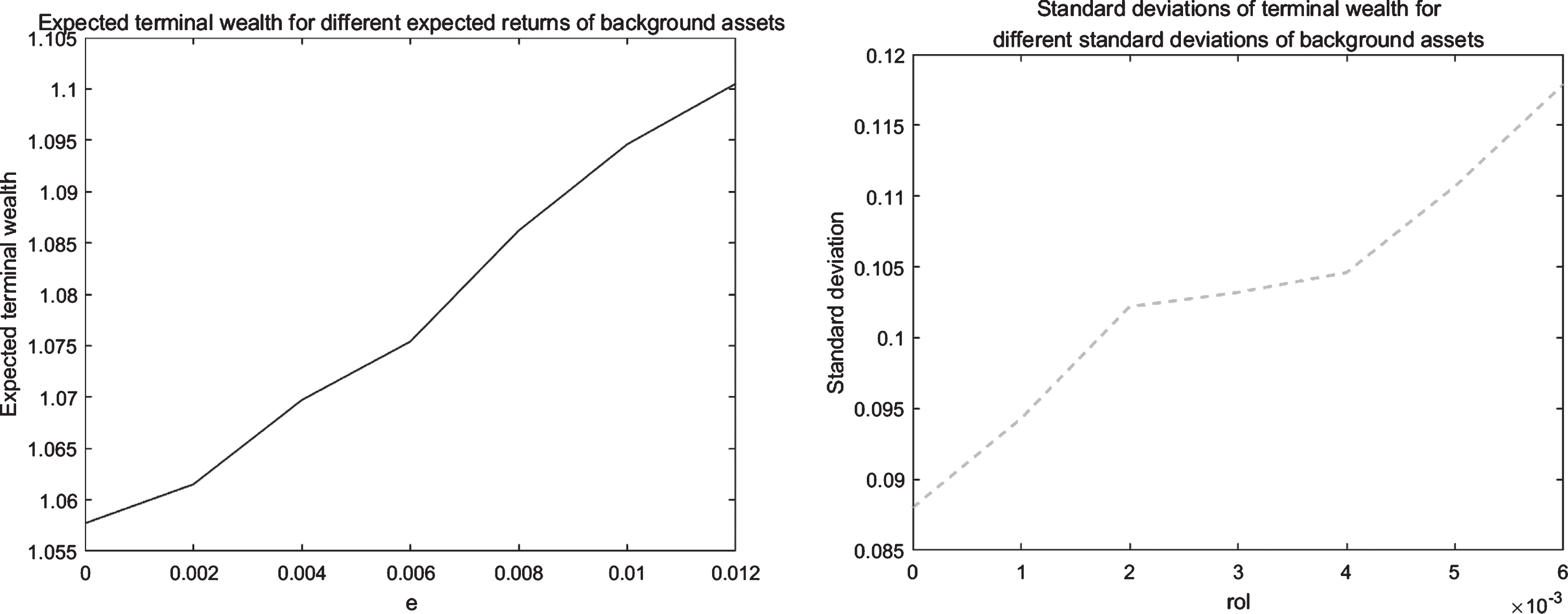
The effect of background assets on the portfolio selection problem.

6 Conclusion

In this paper, we have investigated an uncertain multiperiod portfolio selection problem under the assumption that the return rates are uncertain variables. Considering different criteria, including return, risk, background risk, asset liquidity, transaction costs, and investment proportion restrictions, uncertain multiperiod mean-variance portfolio selection models have been established. We have also converted the optimization models into deterministic forms when the return rates and turnover rates of risky assets were uncertain normal variables. We found that the expected terminal return of the optimal multiperiod portfolio with asset liquidity was greater than that of the optimal multiperiod portfolio without asset liquidity. As the return of the background assets increases, the optimal expected terminal wealth also increases. Meanwhile, the greater the background risk is, the greater the risk of the optimal portfolio. Due to the complexity of the uncertain multiperiod portfolio selection models, we used the genetic algorithm to obtain the numerical solution of the models. This work can be used to help investors make appropriate investment decisions based on their preferences in a complex financial market.

There are many extensions of our paper in the future. One could extend the model to include a multiplicative background asset. In addition, many uncertain multiperiod portfolio selection models with other measures have been developed, and these models could be extended to consider background risk. Background risk can also be added in the uncertain mean-variance-skewness model for portfolio selection.

Footnotes

Acknowledgments

This work was supported by Beijing Natural Science Foundation under [Grant number 9204024].

References

Markowitz

, Portfolio Selection, The Journal of Finance 7(1) (1952), 77–91.

Woodside-Oriakhi

, Lucas

, Beasley

J.E.

, Portfolio rebalancing with an investment horizon and transaction costs, Omega 41 (2013), 406–420.

Kim

, Na

, Higher-moment liquidity risks and the cross-section of stock returns, Journal of Financial Market 38 (2018), 39–59.

Baptista

A.M.

, Optimal delegated portfolio management with background risk, Journal of Banking & Finance 32(6) (2008), 977–985.

Tsanakas

, Risk measurement in the presence of background risk, Insurance: Mathematics and Economics 42(2) (2008), 520–528.

Cocco

J.F.

, Gomes

F.J.

, Maenhout

P.J.

, Consumption and Portfolio Choice over the Life Cycle, Review of Financial Studies 18(2) (2005), 491–533.

Angerer

, Lam

, Income Risk and Portfolio Choice: An Empirical Study, The Journal of Finance 64(2) (2009), 1037–1055.

Cardak

B.A.

, Wilkins

, The determinants of household risky asset holdings: Australian evidence on background risk and other factors, Journal of Banking & Finance 33(5) (2009), 850–860.

Heaton

, Lucas

, Portfolio Choice and Asset Prices: The Importance of Entrepreneurial Risk, The Journal of Finance 55(3) (2000), 1163–1198.

10.

Berkowitz

M.K.

, Qiu

, A further look at household portfolio choice and health status, Journal of Banking & Finance 30(4) (2006), 1201–1217.

11.

Baptista

A.M.

, Portfolio selection with mental accounts and background risk, Journal of Banking & Finance 36(4) (2012), 968–980.

12.

Huang

, Wang

, Portfolio selection and portfolio frontier with background risk, The North American Journal of Economics and Finance 26 (2013), 177–196.

13.

Jiang

, Ma

, An

, An analysis of portfolio selection with background risk, Journal of Banking & Finance 34(12) (2010), 3055–3060.

14.

Guo

, Wagener

, Wong

, Zhu

, The two-moment decision model with additive risks, Risk Management 20(1) (2018), 77–94.

15.

Guo

, Chan

R.H.

, Wong

, Zhu

, Mean-variance, mean-VaR, and mean-CVaR models for portfolio selection with background risk, Risk management (Leicestershire, England) 21(2) (2019), 73–98.

16.

Mossin

, Optimal Multiperiod Portfolio Policies, The Journal of Business 41(2) (1968), 215–229.

17.

Hakansson

N.H.

, Multi-Period Mean-Variance Analysis: Toward a General Theory of Portfolio Choice, The Journal of Finance 26(4) (1971), 857–884.

18.

, Ng

, Optimal Dynamic Portfolio Selection: Multiperiod Mean-variance Formulation, Mathematical Finance 10(3) (2000), 387–406.

19.

Oswaldo Luiz do Valle Costa and Rodrigo de Barros Nabholz, A multi-period mean-variance portfolio selection problem, Brazilian Review of Finance 3(1) (2005), 101–121.

20.

, Takahashi

, Inoue

, Wang

, Dynamic portfolio optimization with risk control for absolute deviation model, European Journal of Operational Research 201(2) (2010), 349–364.

21.

Hakansson

, Optimal Investment and Consumption Strategies Under Risk, an Uncertain Lifetime, and Insurance, International Economic Review 10(3) (1969), 443–466.

22.

Bertsimas

, Pachamanova

, Robust multiperiod portfolio management in the presence of transaction costs, Computers & Operations Research 35(1) (2008), 3–17.

23.

Mei

, DeMiguel

, Nogales

F.J.

, Multiperiod portfolio optimization with multiple risky assets and general transaction costs, Journal of Banking & Finance 69 (2016), 108–120.

24.

Zhang

, Zhang

, Using genetic algorithm to solve a new multi-period stochastic optimization model, Journal of Computational and Applied Mathematics 231(1) (2009), 114–123.

25.

Östermark

, A fuzzy control model (FCM) for dynamic portfolio management, Fuzzy Sets and Systems 78(3) (1996), 243–254.

26.

Huang

, Portfolio selection with fuzzy returns, Journal of Intelligent and Fuzzy Systems 18(4) (2007), 383–390.

27.

Kar

M.B.

, Majumder

, Kar

, Pal

, Cross-entropy based multi-objective uncertain portfolio selection problem, Journal of Intelligent & Fuzzy Systems 32(6) (2017), 4467–4483.

28.

Kar

M.B.

, Kar

, Guo

, Li

, Majumder

, A new bi-objective fuzzy portfolio selection model and its solution through evolutionary algorithms, Soft Computing 23(12) (2019), 4367–4381.

29.

Liu

, Zhang

, Xu

, Fuzzy multi-period portfolio selection optimization models using multiple criteria, Automatica 48(12) (2012), 3042–3053.

30.

Guo

, Yu

, Li

, Kar

, Fuzzy multi-period portfolio selection with different investment horizons, European Journal of Operational Research 254(3) (2016), 1026–1035.

31.

Xiao

, EFMCDM: Evidential fuzzy multicriteria decision making based on belief entropy, IEEE transactions on fuzzy systems 28(7) (2019), 1–1.

32.

Liu

, Why is there a need for uncertainty theory, Journal of Uncertain Systems 6(1) (2012), 3–10.

33.

Liu

, Uncertainty Theory. 2007: Berlin: Springer-Verlag.

34.

Huang

and Yang

, How does background risk affect portfolio choice An analysis based on uncertain mean-variance model with background risk, Journal of Banking and Finance 111 (2020), 105726–.

35.

Huang

, Portfolio Analysis: From Probabilistic to Credibilistic and Uncertain Approaches. 2010: Berlin: Springer-Verlag.

36.

Huang

, Mean-risk model for uncertain portfolio selection, Fuzzy Optimization and Decision Making 10(1) (2011), 71–89.

37.

Huang

, Mean-variance models for portfolio selection subject to experts’ estimations, Expert Systems with Applications 39(5) (2012), 5887–5893.

38.

Huang

, Zhao

, Mean-chance model for portfolio selection based on uncertain measure, Insurance: Mathematics and Economics 59 (2014), 243–250.

39.

Huang

, Di

, Uncertain portfolio selection with background risk, Applied Mathematics and Computation 276 (2016), 284–296.

40.

Huang

, Di

, Uncertain portfolio selection with mental accounts, International Journal of Systems Science 51(12) (2020), 2079–2090.

41.

, Zhu

, Sun

, Aw

, Teo

K.L.

, Multi-period portfolio selection problem under uncertain environment with bankruptcy constraint, Applied Mathematical Modelling 56 (2018), 539–550.

42.

Chen

, Li

, Lu

, Liu

, Multi-period mean-semivariance portfolio optimization based on uncertain measure, Soft Computing 23(15) (2019), 6231–6247.

43.

Zhang

, Multiperiod mean absolute deviation uncertain portfolio selection with real constraints, Soft Computing 23(13) (2019), 5081–5098.

44.

Jin

, Chen

, Yuan

, Multi-period and tri-objective uncertain portfolio selection model: A behavioral approach, The North American Journal of Economics and Finance 47 (2019), 492–504.

45.

Holland

J.H.

, Adaptation in Natural and Artificial Systems. 1975: New York: University of Michigan Press.

46.

Huang

, Zhao

, Kudratova

, Uncertain mean-variance and mean-semivariance models for optimal project selection and scheduling, Knowledge-Based Systems 93 (2016), 1–11.