Fuzzy identification of systems based on adaptive neurons

Abstract

The identification of nonlinear systems is a complex task. This article presents a method comparison between the new Fuzzy Adaptive Neurons (FAN), Radial Basis Function Network (RBF), and Adaptive Network-Based Fuzzy Inference System (ANFIS). The nonlinear systems presented are solved with stable and optimal learning. The simulation of the results for two models presented, are carried out in Matlab^®, the optimization of the system identification for the first and second systems were obtained with great success.

Keywords

Fuzzy adaptive neurons identification of systems learning algorithm level sets ANFIS nonlinear systems

1 Introduction

The identification of systems has required classical (non-fuzzy) and fuzzy methods [1 –8]. In particular, fuzzy methods have used fuzzy neural networks (FNNs) with fuzzy inference rules, and learning algorithms such as backpropagation with Sigmoid and Gaussian Activation Functions [9 –13].

Fuzzy systems require proper activation functions for systems identification [14]. Usually the models proposed with FNNs, to approximate the nonlinear functions include fuzzy inference rules, however, FNNs with adequate activation functions and learning algorithms are required to successfully solve the precision problems in fuzzy identification of the system.

Fuzzy Adaptive Neurons (FANs) are based on fuzzy logic [9, 15], and the model of fuzzy neurons of Gupta [3 –5]. The FAN is a new method because in [16 –19] was developed a new Sigmoid Activation Function and a learning algorithm based on error correction. FAN method has been successfully applied at parameter identification based on force and moment data [7], to the neuro-fuzzy design of control law for a PID controller [20, 21], to trajectory tracking control of a multi-rotor unmanned aerial vehicle based on experimental aerodynamic data [22], for earthquake modeling with seismic accelerograms [23], and for recognition and processing of spatiotemporal spike patterns [8, 24].

Membership functions with different shapes, such as triangular, trapezoidal, sigmoidal, bell, Gaussian, among others, have been proposed depending on the application [25].

In [26] presents a fractional fuzzy inference system (FFIS), based on fractional membership functions with fractional indices constant or dynamic. Fractional membership functions are defined by level sets, with applications to predict chaotic time series and a fuzzy closed loop control system. FAN’s sigmoid membership function use a constant or dynamical threshold, based on level sets. The threshold defines the left or lower level set of the somatic aggregation operation fuzzy set.

Applications for parameter identification of dynamic systems with artificial neural networks (ANN) and ANFIS have been proposed in [27], to define parameters of dynamic equations for dynamic and control analysis. Based on input data the ANN and ANFIS to estimate the unknown parameters.

The novel FANs learning algorithm performs system identification in a stable and optimal way [7 , 20–24]. This article proposes a method comparison between Radial Basis Function Network (RBF), Adaptive Network-Based Fuzzy Inference System (ANFIS) and FAN. In [23] the modeling is based on axon delays that produce a phase shift at the output with respect to the input of the system, and a new Gaussian activation function (GAF) for fuzzy systems. The methods presented here develop the models with some delayed inputs and delayed feedback outputs.

The article is organized in the following sections, Section 2, describes the FANs model and the learning algorithm, developed in [16–19 , 22–24], for fuzzy unipolar and bipolar systems.

Section 3 presents the modeling of two nonlinear systems. The first model is solved based on fuzzy neural modeling with FANs and ANFIS. A second model is developed by four methods with the purpose of comparing the results, using the learning algorithm for error correction for FANs. The first method is sigmoid activation function (SAF-FANs), the second is a Radial Based Function (RBF), the third is through ANFIS, and the fourth method is the learning algorithm of the FANs.

Section 4 presents a comparative analysis between ANFIS and FAN learning algorithms. Also the stability analysis of SAF-FAN model 1 and FAN model 2.

In Section 5 shows the simulation results in Matlab^® of two models. Model 1 is a two-dimensional function. Model 2 is nonlinear plant.

Section 6 presents the conclusions and future challenges.

2 Preliminaries

Different models of fuzzy neurons have been established [3–5 , 16–19], here the Fuzzy Adaptive Neurons model is described.

2.1 Fuzzy adaptive neurons

A synaptic operation, a somatic Gupta-type aggregation or fuzzy integrator operation, and a nonlinear somatic operation with its learning algorithm for fuzzy systems [16–19 , 22–24] conjoin the model of FANs. Synaptic operation, (1), aggregation operation, (2), (3) are the somatic operations. ${\tilde{V}}_{minj} (k) = min (z_{inj} (k), w_{inj} (k))$ (1) ${\tilde{V}}_{\max} (k) = {MAX}_{j = 1}^{N} {\tilde{V}}_{minj} (k)$ (2) ${\tilde{V}}_{out} (k) = max ({\tilde{V}}_{\max} (k), V_{threshold} (k))$ (3) ${\tilde{V}}_{γ} (k) = \min (γ, {\tilde{V}}_{out} (k))$ (4)

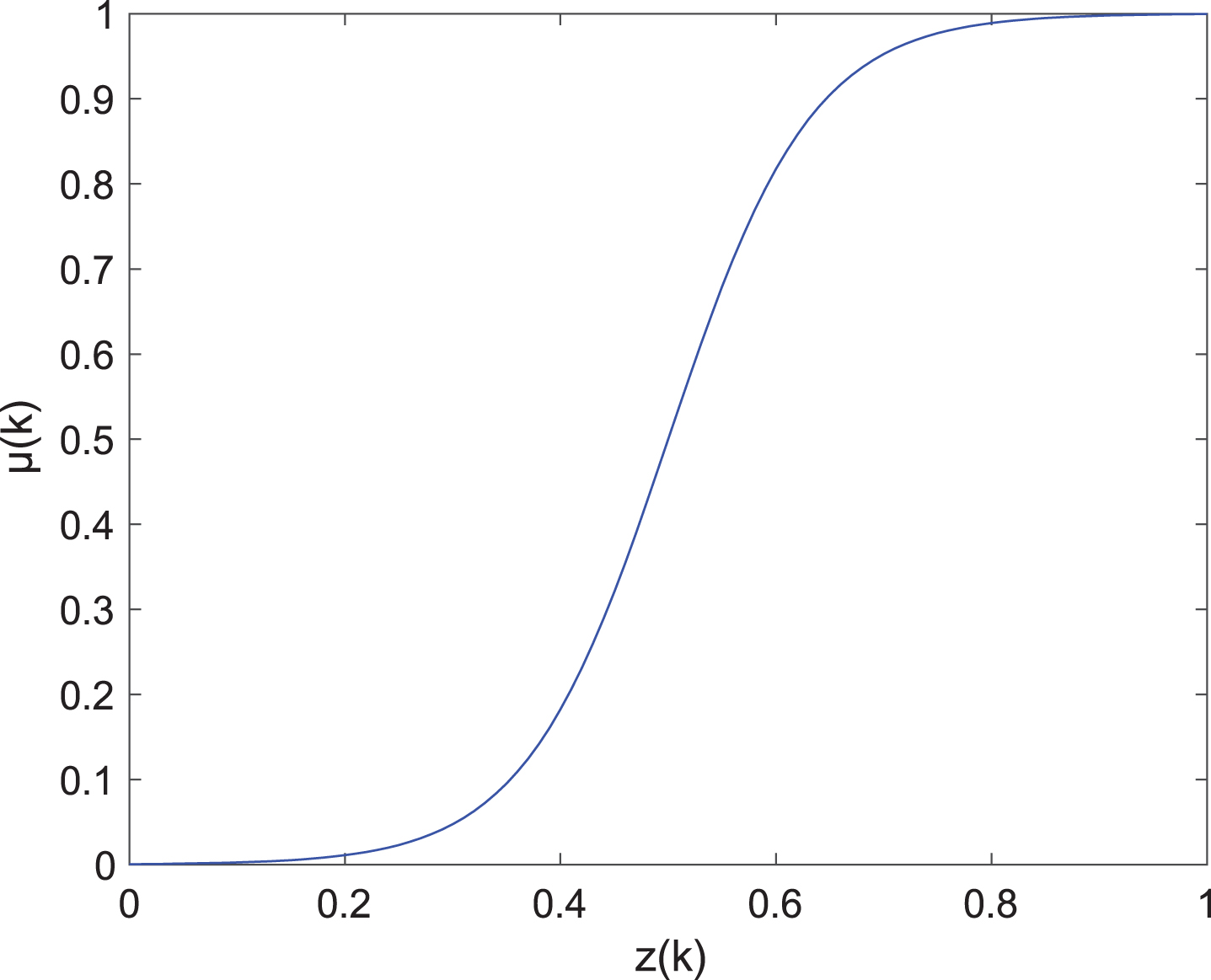
Fuzzy unipolar systems are within the interval [0,1], then the nonlinear operation with threshold is defined in (3–5), Fig. 1. The learning algorithm is shown in (6–8), $\tilde{y} (k) = \frac{1}{1 + e^{(- {\tilde{V}}_{γ} (k) \cdot a + b)}}$ (5) $e (k) = {\tilde{y}}_{ref} (k) - \tilde{y} (k)$ (6) $γ (k + 1) = γ (k) + Δ γ (k)$ (7) $w_{inj} (k + 1) = w_{inj} (k) + Δ w_{inj} (k)$ (8)

Fig. 1

Sigmoid Activation Function or membership function for unipolar systems.

Where:

k time variable.

a 0 < a

b 0 < b

e (k) error.

γ (k) learning factor, 0 < γ ⩽ 1.

V_threshold (k) threshold.

z_inj (k) dendrite inputs.

w_inj (k) synaptic weights.

$\tilde{y} (k)$ sigmoid activation function (SAF).

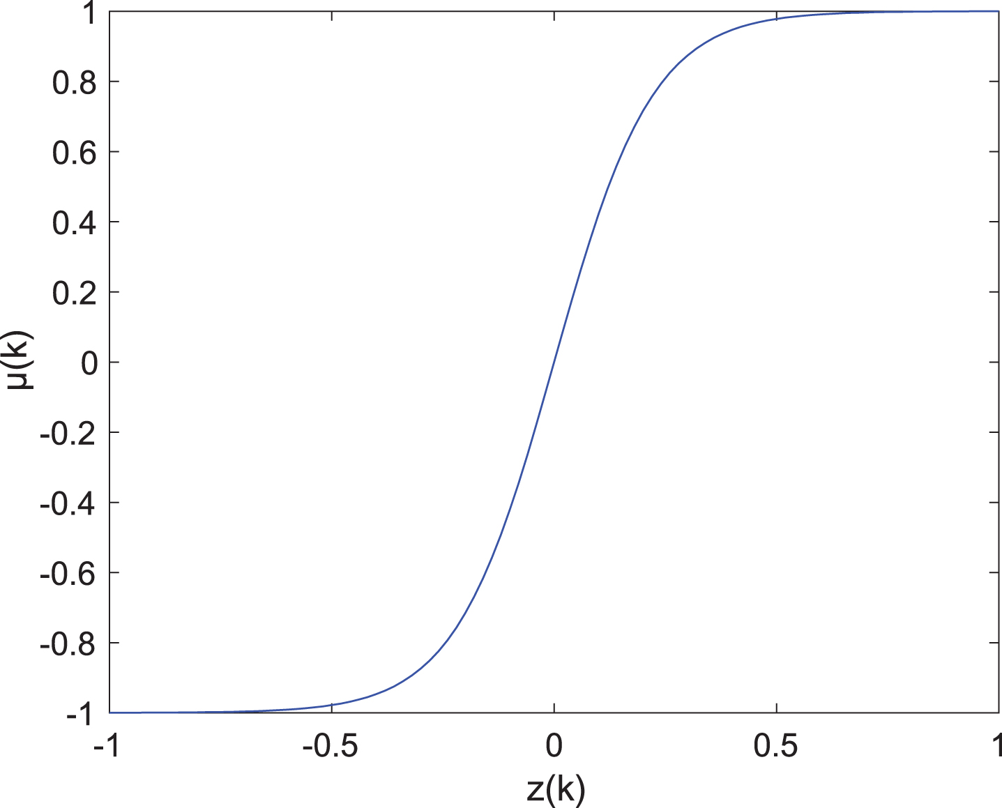
Fuzzy bipolar systems are within the interval [–1,1]. Nonlinear operation with threshold is defined in (9), Fig. 2 and the learning algorithm in (10–12), $\tilde{y} (k) = \frac{2}{1 + e^{(- {\tilde{V}}_{γ} (k) \cdot c)}} - 1$ (9) $e (k) = {\tilde{y}}_{ref} (k) - \tilde{y} (k)$ (10) $γ (k + 1) = γ (k) + Δ γ (k)$ (11) $w_{inj} (k + 1) = w_{inj} (k) + Δ w_{inj} (k)$ (12) Where:

Fig. 2

Sigmoid Activation Function or membership function for bipolar systems.

k time variable.

c 0 < c

e (k) error.

γ (k) learning factor, -1 < γ ⩽ 1.

V_threshold (k) threshold.

z_inj (k) dendrite inputs.

w_inj (k) synaptic weights.

$\tilde{y} (k)$ sigmoid activation function (SAF).

2.1.1 Level sets

If ${\tilde{V}}_{\max}$ is a fuzzy mapping from U to V, for any α = V_threshold

α ∈[0, 1] for unipolar systems

α ∈[-1, 1] for bipolar systems

Then, an ordinary multimapping ${\tilde{V}}_{\max_{α}} = {\tilde{V}}_{out}$ could be defined as follows, $\forall u \in U {\tilde{V}}_{\max_{α}} (u) = {v | μ_{{\tilde{V}}_{\max} (u)} (v) ⩾ α} \subseteq V$ (13)

${\tilde{V}}_{\max_{α}}$ can be an α-cut or level set of ${\tilde{V}}_{\max}$ [15].

${\tilde{V}}_{\max_{α}}$ could be viewed as a crisp subset of V^U, i.e. a set of mappings, $\begin{matrix} {\tilde{V}}_{\max_{α}} \\ = {V_{\max} : U \to V | \forall u \in U, V_{\max} (u) \in {\tilde{V}}_{\max_{α}} (u)} \\ = {V_{\max} : U \to V | inf_{u \in U} μ_{{\tilde{V}}_{\max} (u)} (V_{\max} (u)) ⩾ α} \end{matrix}$ (14)

${\tilde{V}}_{\max_{α}}$ is the α-cut of a fuzzy set of mappings (FSM) generated by ${\tilde{V}}_{\max}$ , a good crisp representation of ${\tilde{V}}_{\max} : V_{\max}$ a good representation of ${\tilde{V}}_{\max}$ ∀u ∈ U|V_max (u) matches ${\tilde{V}}_{\max} (u)$ sufficiently.

$ht ({\tilde{V}}_{\max})$ denotes the height of the fuzzy set ${\tilde{V}}_{\max}$ $ht ({\tilde{V}}_{\max}) = sup μ_{{\tilde{V}}_{\max} (u)}$ , the greatest membership value of an element in ${\tilde{V}}_{\max}$ then, ∀α > 0 $if \forall u \in U ht ({\tilde{V}}_{\max} (u)) ⩾ α, then ht ({\tilde{V}}_{\max_{α}}) ⩾ α$ $if \exists u \in U ht ({\tilde{V}}_{\max} (u)) < α, then ht ({\tilde{V}}_{\max_{α}}) < α$

However, for FANs is possible to stablish a height with a second threshold α⁺, (16) based on (3), therefore threshold in (3) can be expressed as α^-, (15), ${\tilde{V}}_{\max_{α^{-}}} (k) = max ({\tilde{V}}_{\max} (k), α^{-} (k))$ (15) ${\tilde{V}}_{\max_{α^{+}}} (k) = min ({\tilde{V}}_{\max_{α^{-}}} (k), α^{+} (k))$ (16)

Where, α^- ⩽ α⁺.

2.2 Adaptive network-based fuzzy inference system

A system with fuzzy inference rules, membership functions, and adaptive neural networks define ANFIS, based on Mamdani and Takagi-Sugeno-Kang (TSK) fuzzy models [10].

Based on Mamdani fuzzy model and expressing by inference product and a fuzzifier, the p output of the fuzzy logic system, $\begin{matrix} R^{i} : IF x_{1} is A_{1 i} and x_{2} is A_{2 i} and \dots x_{n} is A_{ni} \\ THEN {\hat{y}}_{1} is B_{1 i} and \dots {\hat{y}}_{m} is B_{mi} \end{matrix}$ (17)

Where i = 1, 2, …, l, $X = [x_{1} \dots x_{n}] \in R^{n}, \hat{Y} (k) = {[{\hat{y}}_{1} \dots {\hat{y}}_{m}]}^{T} \in R^{m \times 1}, A_{1 i}, \dots, A_{ni}$ and B_1i, ⋯ , B_mi are standard fuzzy sets. ${\hat{y}}_{p} = \frac{(\sum_{i = 1}^{l} w_{pi} [\prod_{j = 1}^{n} μ_{A_{ji}}])}{\sum_{i = 1}^{l} [\prod_{j = 1}^{n} μ_{A_{ji}}]} = \sum_{i = 1}^{l} w_{pi} \cdot φ_{i}$ (18)

Where μ_{A
_ji} is the membership functions of the fuzzy sets A_ji. In [10] we defined, $φ_{i} = \frac{\prod_{j = 1}^{n} μ_{A_{ji}}}{\sum_{i = 1}^{l} [\prod_{j = 1}^{n} μ_{A_{ji}}]}$ (19) $\hat{Y} (k) = W (k) \cdot Φ [X (k)]$ (20)

Where parameters $W (k) = [\begin{matrix} w_{11} & w_{1 l} \\ ⋱ \\ w_{m 1} & w_{ml} \end{matrix}] \in R^{m \times l}$ , data vector $Φ [X (k)] = {[φ_{i} \dots φ_{l}]}^{T} \in R^{l \times 1}$ . A learning algorithm is, $W (k + 1) = W (k) - η \cdot e (k) \cdot Φ^{T} [X (k)]$ (21)

Where 0 < η ⩽ 1.

A Takagi-Sugeno-Kang fuzzy model, $\begin{matrix} R^{i} : IF x_{1} is A_{1 i} and x_{2} is A_{2 i} and \dots x_{n} is A_{ni} \\ THEN {\hat{y}}_{j} = p_{j 0}^{i} + p_{j 1}^{i} x_{1} + \dots + p_{jn}^{i} x_{n} \end{matrix}$ (22)

Where j = 1, 2, …, m. $X = [x_{1} \dots x_{n}] \in R^{n}, \hat{Y} (k) = {[{\hat{y}}_{1} \dots {\hat{y}}_{m}]}^{T} \in R^{m \times 1}, A_{1 i}, \dots, A_{ni}$ and B_1i, ⋯ , B_mi are standard fuzzy sets. ${\hat{y}}_{q} = \sum_{i = 1}^{l} (p_{q 0}^{i} + p_{q 1}^{i} x_{1} + \dots + p_{qn}^{i} x_{n}) \cdot φ_{i}$ (23)

Where φ_i is defined in (19). Expressing (23) in the form of Mamdani-type, $\hat{Y} (k) = W (k) \cdot Φ [X (k)]$ (24)

Where $\hat{Y} (k) = {[{\hat{y}}_{1} \dots {\hat{y}}_{m}]}^{T}$ $W (k) = [\begin{matrix} p_{10}^{1} & p_{q 0}^{l} \\ ⋱ \\ p_{m 0}^{1} & p_{m 0}^{l} \end{matrix} \begin{matrix} p_{11}^{1} & p_{11}^{l} \\ ⋱ \\ p_{m 1}^{1} & p_{m 1}^{l} \end{matrix} \begin{matrix} p_{1 n}^{1} & p_{1 n}^{l} \\ ⋱ \\ p_{mn}^{1} & p_{mn}^{l} \end{matrix}]$ $Φ [X (k)] = {[φ_{1} \dots φ_{l} x_{1} φ_{1} \dots x_{1} φ_{l} x_{n} φ_{1} \dots x_{n} φ_{l}]}^{T}$

A TSK-type fuzzy neural model with Gaussian membership functions, the q output of the fuzzy logic system is, $\begin{matrix} {\hat{y}}_{q} = \frac{(\sum_{i = 1}^{l} w_{qi} [\prod_{j = 1}^{n} μ_{A_{ji}}])}{\sum_{i = 1}^{l} [\prod_{j = 1}^{n} μ_{A_{ji}}]} \\ = \frac{(\sum_{i = 1}^{l} w_{qi} [\prod_{j = 1}^{n} \exp (- \frac{{(x_{j} - c_{ji})}^{2}}{σ_{ji}^{2}})])}{\sum_{i = 1}^{l} [\prod_{j = 1}^{n} \exp (- \frac{{(x_{j} - c_{ji})}^{2}}{σ_{ji}^{2}})]} \end{matrix}$ (25)

$r_{i} = \prod_{j = 1}^{n} \exp (- \frac{{(x_{j} - c_{ji})}^{2}}{σ_{ji}^{2}})$ ; $a_{q} = \sum_{i = 1}^{l} w_{qi} r_{i}$ ; $b_{q} = \sum_{i = 1}^{l} r_{i}$ ; ${\hat{y}}_{q} = \frac{a_{q}}{b_{q}}$

A learning algorithm is, $p_{qk}^{i} (k + 1) = p_{qk}^{i} (k) - η \cdot ({\hat{y}}_{q} - y_{q}) \cdot \frac{r_{i}}{b_{q}} \cdot x_{k}$ (26) $\begin{matrix} c_{ji} (k + 1) = c_{ji} (k) - 2 \cdot η \cdot r_{i} \cdot \frac{w_{pi} - {\hat{y}}_{p}}{b_{q}} \\ \cdot \frac{x_{j} - c_{ji}}{σ_{ji}^{2}} \cdot ({\hat{y}}_{q} - y_{q}) \end{matrix}$ (27) $\begin{matrix} σ_{ji} (k + 1) = σ_{ji} (k) - 2 \cdot η \cdot r_{i} \cdot \frac{w_{pi} - {\hat{y}}_{p}}{b_{q}} \\ \cdot \frac{{(x_{j} - c_{ji})}^{2}}{σ_{ji}^{3}} \cdot ({\hat{y}}_{q} - y_{q}) \end{matrix}$ (28)

Where 0 < η ⩽ 1.

3 Fuzzy neural modeling with adaptive neurons

Based on inputs-outputs information of the identified plant/function, we develop a model with FANs, for system identification and obtain a model with fixed weights, models 1-2.

Neuronal fuzzy modeling allows us to approximate $\hat{y} (k)$ to output y (k) of a system with X (k) inputs, through online weight training, of a system with FANs. $Plant : y = W^{*} \cdot Φ [H (k)]$ (29) $Model : \hat{y} = W (k) \cdot Φ [H (k)]$ (30) $Error : y - \hat{y} = (W^{*} - W (k)) \cdot Φ [H (k)]$ (31)

Where Φ [·] is a function. For model 1 H (k) = X (k). For model 2, the NARMA (nonlinear autoregressive movement average) model [10], the multivariable NARMA form, where H (k) = [Y (k - d_t) , …, U (k - d_t) , …] ^T. Where d_t is a time delay.

3.1 Model 1

A model $\hat{f} (k)$ is proposed to identify a bi-dimensional function f (k). $\hat{F} (k) = W (k) (v_{1} + x_{1} (k) + x_{2} (k) + Φ [x_{1} (k), x_{2} (k)])$ (32)

Where v₁ is a constant.

In [10] we used the fuzzy neural network (18), here we propose, $\begin{matrix} {\hat{y}}_{model 1} = \frac{(\sum_{i = 1}^{l} w_{i} \cdot z_{in ANFISi} \cdot [\prod_{j = 1}^{n} μ_{A_{ji}}])}{\sum_{i = 1}^{l} [\prod_{j = 1}^{n} μ_{A_{ji}}]} \\ {\hat{y}}_{model 1} = \sum_{i = 1}^{l} w_{i} \cdot z_{in ANFISi} \cdot φ_{i} \end{matrix}$ (33)

Where $z_{in ANFISi} = {\hat{y}}_{i} (X (k))$ .

3.2 Model 2

Nonlinear system identification is based on four methods to compare, we define the approximation with the proposed model (34) for the SAF-FANs method (4–7), RBF-NN method, ANFIS method and the learning algorithm for fuzzy systems. For FANs method, the models (35–38) is proposed, $\hat{y} (k) = W (k) \cdot Φ [H (k)]$ (34) $\begin{matrix} {\hat{y}}_{SAF - FANs} (k) = W (k) \cdot (H (k) + W (k)) + W (k) \\ \cdot H (k) + W (k) \cdot H (k) \cdot v_{2} \end{matrix}$ (35) $\begin{matrix} {\hat{y}}_{RBF - NN} (k) = (W (k) \cdot μ_{1} [k] + W (k) \cdot μ_{2} [k] \\ + H (k)) \cdot Φ [k] \end{matrix}$ (36) ${\hat{y}}_{ANFIS} (k) = Φ [k] \cdot (W (k) \cdot H^{T} (k) + v_{3}) \cdot v_{4}$ (37) $\begin{matrix} {\hat{y}}_{FANs} (k) = (W (k) \cdot W^{T} (k) \cdot H (k) + H (k) + W (k) \\ - v_{5} \cdot (W (k) \cdot W^{T} (k) \cdot H (k) + H (k) \cdot v_{6} + W (k)) \\ + v_{7} \cdot (W (k) \cdot W^{T} (k) \cdot H (k) + H (k) \cdot v_{8} + W (k))) \\ \cdot v_{9} \cdot Φ [k] \end{matrix}$ (38)

Where v₂ · sv₉ are a constant.

In [10] we used the fuzzy neural network (25), here we propose, ${\hat{y}}_{model 2} = \frac{(\sum_{i = 1}^{l} w_{i} \cdot z_{in ANFISi} \cdot [\prod_{j = 1}^{n} μ_{A_{ji}}])}{\sum_{i = 1}^{l} [\prod_{j = 1}^{n} μ_{A_{ji}}]}$ (39) $\begin{matrix} {\hat{y}}_{model 2} = \\ \frac{(\sum_{i = 1}^{l} w_{i} \cdot z_{in ANFISi} \cdot [\prod_{j = 1}^{n} \exp (- \frac{{(z_{in ANFISj} - c_{ji})}^{2}}{σ_{ji}^{2}})])}{\sum_{i = 1}^{l} [\prod_{j = 1}^{n} \exp (- \frac{{(x_{j} - c_{ji})}^{2}}{σ_{ji}^{2}})]} \end{matrix}$ (40)

Where $z_{in ANFISi} = {\hat{y}}_{2 i} (X (k))$ .

4 Theoretical analysis

4.1 Comparison between the learning algorithm of the ANFIS and the FAN

A model $\hat{f} (k)$ is proposed to identify a bi-dimensional.

The learning algorithms of the ANFIS and FANs are similar because they are both use the error correction method.

The comparison analysis is based on the equations to update the weights and their operating intervals of the parameters [19 , 28–31], for example, the learning factor.

Equation (21) defines weight training for ANFIS, and (38) developed, defined and presented in [19 , 23] for FANs. $w_{FAN} (k + 1) = w_{FAN} (k) + γ (k) \cdot e (k) \cdot Φ^{T} [x (k)]$ (41) $γ (k + 1) = γ (k) + γ (k) \cdot e (k) \cdot Φ^{T} [x (k)]$ (42)

For both algorithms, the learning factors 0 < η ⩽ 1 and 0 < γ ⩽ 1 are bounded. However, ANFIS (21) applies to both unipolar [0, 1] and bipolar [–1, 1] intervals. FAN (41) is limited for unipolar an bipolar intervals.

ANFIS learning algorithm for unipolar input-output can also take bipolar values. FANs are bounded for unipolar and bipolar values. Therefore, the error is more bounded in the FAN learning algorithm,

For bipolar input-output, from (21),

If w_ANFIS (k) = -1, η · e (k) · Φ^T [X (k)] = 1 then w_ANFIS (k + 1) = -2.

From (38), If w_FAN (k) = -1, γ · e (k) · Φ^T [X (k)] = -1.

Then w_FAN (k + 1) = -2. Due to bounded conditions,

-1 ⩽ w_FAN (k + 1) ⩽ 1, ∴ w_FAN (k + 1) = -1. Therefore,

w_FAN (k + 1) ⩽ w_ANFIS (k + 1), the FAN learning algorithm for fuzzy systems has more bounded parameters than that of the ANFIS.

4.2 Stability analysis

Nonlinear systems in discrete time can be expressed as (32) for model 1 and (38) for model 2, in matrix form. Then,

Model 1 $\begin{matrix} F (k) = W^{*} (v_{1} + \sum X (k) + Φ [X (k)]) + W_{d}^{*} \\ (v_{1 d} + \sum X_{d} (k) + Φ [X_{d} (k)]) + d (t) \end{matrix}$ (43)

Where W^* are the unknown weights to minimize the unmodeled dynamic $W_{d}^{*} (v_{1 d} + \sum X_{d} (k) + Φ [X_{d} (k)])$ , d (t) is the unmodeled dynamic.

Identification error of FAN training method in matrix form, is defined as, $E (k) = F (k) - \hat{F} (k)$ (44) $\begin{matrix} E (k) = W^{*} (v_{1} + \sum X (k) + Φ [X (k)]) \\ + W_{d}^{*} (v_{1 d} + \sum X_{d} (k) + Φ [X_{d} (k)]) \\ - W (v_{1} + \sum X (k) + Φ [X (k)]) \end{matrix}$ (45) $\begin{matrix} E (k) = \tilde{W} (v_{1} + \sum X (k) + Φ [X (k)]) \\ + W_{d}^{*} (v_{1 d} + \sum X_{d} (k) + Φ [X_{d} (k)]) \end{matrix}$ (46) $E (k) = \tilde{W} (v_{1} + \sum X (k) + Φ [X (k)]) + η_{d}$ (47)

Where, $\tilde{W} = W^{*} - W$ , and $η_{d} = W_{d}^{*} (v_{1 d} + \sum X_{d} (k) + Φ [X_{d} (k)])$ .

From (41) and (42), $W (k + 1) = W (k) + Γ (k) \cdot E (k) \cdot Φ^{T} [X (k)]$ (48) $Γ (k + 1) = Γ (k) + Γ (k) \cdot E (k) \cdot Φ^{T} [X (k)]$ (49)

For open-loop systems identification, it is assumed model 1 and model 2 are bounded-input-bounded-output (BIBO) stable, i.e. y (k) and x (k) at model 1, are bounded. Membership function μ_SAF [·] is bounded. The stability analysis for nonlinear system modeling based on the novel FAN method is given by the following theorem.

Theorem: If unknown nonlinear systems model 1 and model 2, (30), are modeled by the fuzzy systems (32) and (38), the weights are updated by (48) and (49), then the modeling error e (k) is uniformly ultimately bounded (UUB). The normalized identification error is, $E_{N} (k) = \frac{W_{N} (k + 1) - W_{N} (k)}{Γ_{N} (k) \cdot Φ^{T} [X (k)]}$ (50)

Satisfies the following average performance, $\begin{matrix} lim_{T \to \infty} sup \frac{1}{T} \sum_{k = 1}^{T} | | E_{N} (k) | |^{2} ⩽ \max_{k} \\ [| | W_{d}^{*} (v_{1 d} + \sum X_{d} (k) + Φ [X_{d} (k)]) | |^{2}] \end{matrix}$ $lim_{T \to \infty} sup \frac{1}{T} \sum_{k = 1}^{T} | | E_{N} (k) | |^{2} ⩽ η_{d}$ (51)

Proof:

For bipolar systems with values at interval [–1,1],

-1 ⩽ W (k + 1) ⩽ 1

-1 < Γ (k + 1) ⩽ 1

A positive defined scalar L_k is selected, $L_{k} = | | \tilde{W} (k) | |^{2}$ (52) where ∥· ∥ denotes the Euclidean norm.

By the updating law (48), we have, $\tilde{W} (k + 1) = \tilde{W} (k) + Γ (k) \cdot E (k) \cdot Φ^{T} [X (k)]$ (53)

Using the inequalities, $| | q + r | | ⩽ | | q | | + | | r | |, | | q \cdot r | | = | | q | | \cdot | | r | |$

For any “q’’ and “r’’. By using (46) and (53), with -1 < Γ_N (k) ⩽ Γ (k) ⩽1, we have, $\begin{matrix} Δ L_{k} = L_{k + 1} - L_{k} \\ = | | \tilde{W} (k) + Γ (k) \cdot E (k) \cdot Φ^{T} [X (k)] | |^{2} - | | \tilde{W} (k) | |^{2} \\ = 2 | | Γ (k) \cdot E (k) \cdot Φ^{T} [X (k)] \cdot \tilde{W} (k) | | + | | Γ (k) \cdot \\ E (k) \cdot Φ^{T} [X (k)] | |^{2} \\ = | | Γ (k) | |^{2} \cdot | | E (k) | |^{2} \cdot | | Φ^{T} [X (k)] | |^{2} \\ + 2 | | Γ (k) \cdot E (k) \cdot Φ^{T} [X (k)] \\ \cdot \frac{E (k) - W_{d}^{*} (v_{1 d} + \sum X_{d} (k) + Φ [X_{d} (k)])}{(v_{1} + \sum X (k) + Φ [X (k)])} | | \\ = | | Γ (k) | |^{2} \cdot | | E (k) | |^{2} \cdot | | Φ^{T} [X (k)] | |^{2} \\ + \frac{2 | | Γ (k) | | \cdot | | E (k) | |^{2} \cdot | | Φ^{T} [X (k)] | |}{| | (v_{1} + \sum X (k) + Φ [X (k)]) | |} \\ \frac{2 | | Γ (k) | | \cdot | | E (k) | | \cdot | | Φ^{T} [X (k)] | |}{| | (v_{1} + \sum X (k) + Φ [X (k)]) | |} \cdot W_{d}^{*} \\ \cdot (v_{1 d} + \sum X_{d} (k) + Φ [X_{d} (k)]) \end{matrix}$ $\begin{matrix} Δ L_{k} ⩽ ζ (k) \cdot | | E (k) | |^{2} - δ (k) \cdot | | E (k) | | \\ \cdot | | W_{d}^{*} \\ \cdot (v_{1 d} + \sum X_{d} (k) + Φ [X_{d} (k)]) | | \end{matrix}$ $Δ L_{k} ⩽ ζ (k) \cdot | | E (k) | |^{2} - δ (k) \cdot | | E (k) | | \cdot | | η_{d} | |$ (54)

Where ζ (k) and δ (k) are defined as, $\begin{matrix} ζ (k) = | | Γ (k) | |^{2} \cdot | | Φ^{T} [X (k)] | |^{2} \\ + \frac{2 | | Γ (k) | | \cdot | | Φ^{T} [X (k)] | |}{| | (v_{1} + \sum X (k) + Φ [X (k)]) | |} \end{matrix}$ $\begin{matrix} δ (k) = \frac{2 | | Γ (k) | | \cdot | | Φ^{T} [X (k)] | |}{| | (v_{1} + \sum X (k) + Φ [X (k)]) | |} \end{matrix}$ Because, $n min ({\tilde{w}}_{i}^{2}) ⩽ L_{k} ⩽ n max ({\tilde{w}}_{i}^{2})$

Where $n min ({\tilde{w}}_{i}^{2})$ and $n max ({\tilde{w}}_{i}^{2})$ are $K_{\infty} - functions$ , and ζ (k) · ||E (k) ||² is a $K_{\infty} - function$ , δ (k) · ||η_d|| is a $K - function$ . So, L_k admits an ISS-Lyapunov function [10], the dynamic of the identification error is input-to-state stable.

From (43) and (52) we know L_k is the function of E (k) and $W_{d}^{*} (v_{1 d} + \sum X_{d} (k) + Φ [X_{d} (k)])$ . The “INPUT” and the “STATE” correspond to both terms of (35). However, usually, Φ [X_d (k)] ⪡ Φ [X (k)].

Because the “INPUT” is bounded and the dynamic is ISS, therefore the “STATE” E (k) is bounded.

Applying the bounded conditions for W_N (k + 1) and Γ_N (k + 1), Equation (54), from 1 up to T and using 0 < L_T and L₁ is a constant, we obtain, $\begin{matrix} L_{T} - L_{1} ⩽ ζ_{N} (k) \cdot (\sum_{k = 1}^{T} | | E_{N} (k) | |^{2}) - δ_{N} (k) \\ \cdot (\sum_{k = 1}^{T} | | E_{N} (k) | |) \cdot {\bar{η}}_{d} \end{matrix}$ $\begin{matrix} ζ_{N} (k) = | | Γ_{N} (k) | |^{2} \cdot | | Φ^{T} [X (k)] | |^{2} \\ + \frac{2 | | Γ_{N} (k) | | \cdot | | Φ^{T} [X (k)] | |}{| | (v_{1} + \sum X (k) + Φ [X (k)]) | |} \end{matrix}$ $\begin{matrix} δ_{N} (k) = \frac{2 | | Γ_{N} (k) | | \cdot | | Φ^{T} [X (k)] | |}{| | (v_{1} + \sum X (k) + Φ [X (k)]) | |} \end{matrix}$ $\begin{matrix} ζ_{N} (k) \cdot (\sum_{k = 1}^{T} | | E_{N} (k) | |^{2}) \\ ⩽ L_{T} - L_{1} + δ_{N} (k) \cdot (\sum_{k = 1}^{T} | | E_{N} (k) | |) \cdot {\bar{η}}_{d} \end{matrix}$ (55) (51) is established.

Remark 1. To obtain high modeling accuracy for classical fuzzy neural networks, the main difficulty is deciding the parameters. However the novel fuzzy system with adaptive neurons has less parameters to be chosen. And the modeling error converges to the zone ${\bar{η}}_{d}$ .

Remark 2. If the fuzzy system (30) could match the nonlinear plant (29) exactly (if η_d (k) =0), i.e., it could find the best W^* such that the nonlinear system could be expressed as F (k) = W^* (v₁ + ∑X (k) + Φ [X (k)]), the same learning law makes the identified error E (k) asymptotically stable $lim_{K \to \infty} | | E (k) | | = 0$ (56)

Remark 3. The normalization of the learning rates in (43) and (47), are time-varying in order to insure the stability of identification error. The learning rates are easier to be reached than [10]. Because the initial condition does not need any previous information, the time-varying learning rates are usually robust.

5 Simulation

This section presents the proposed stable and optimal learning algorithms with ANFIS and SAF-FAN for model 1 and SAF-FAN, RBF-NN, ANFIS and the FAN learning algorithm, applied to the approximation of functions and identification of nonlinear systems [10]. For model 2 the weights w_i are obtained with the error correction learning algorithm for fuzzy systems [19, 21].

5.1 Model 1. Two-dimensional function approximation

The proposed model in (32), approximates the following nonlinear function: $f (x_{1}, x_{2} = 0.52 + 0.1 \cdot x_{1} + 0.28 \cdot x_{2} - 0.6 \cdot x_{1} \cdot x_{2}$ (57)

We use SAF-FANs (9), for function approximation. The number of input variables is 2. To train the model, 300 data were used, T = 300, the training data selected were, x₁ (k) = -1 + 2k/T, x₂ (k) =1 - 2k/T, k = 1, 2, ·⋯, T. After training and leaving the weights fixed, the simulation results of the function identification are shown in Fig. 3. The error for weight training online, for finite time is defined as, $e (k) = f (k) - \hat{f} (k)$ .

Fig. 3

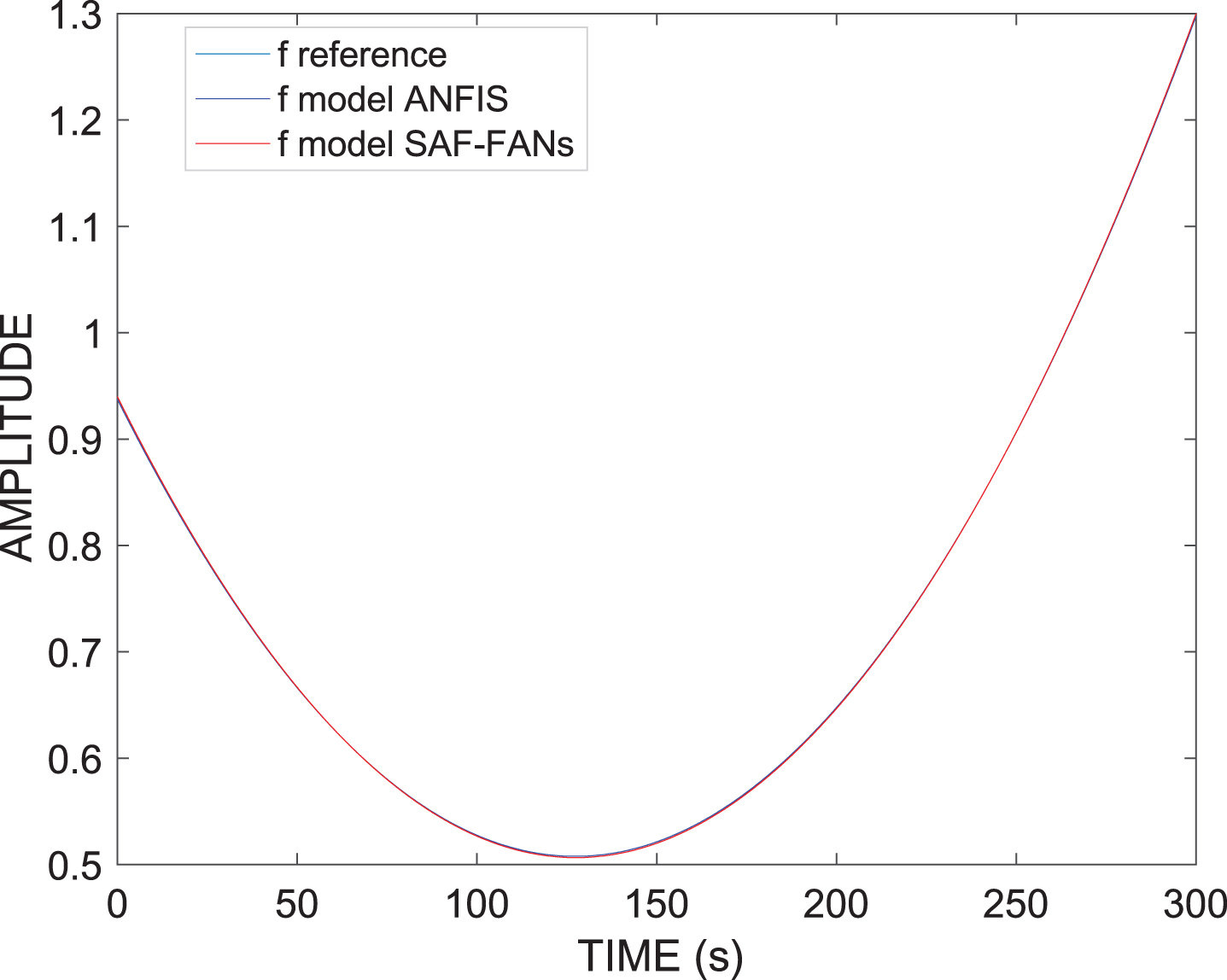
Model 1, Two-Dimensional Function Approximation with ANFIS and SAF-FANs.

From (32), for this two-dimensional system we propose the following standard form, $\begin{matrix} \hat{f} (k) = w_{in 11} + w_{in 21} \cdot x_{1} (k) + w_{in 31} \cdot x_{2} (k) \\ + w_{in 41} \cdot x_{1} (k) \cdot x_{2} (k) \end{matrix}$ (58)

We use the ANFIS and SAF-FANs for modeling the nonlinear plant, Fig. 3. The error after training is defined for finite time as, $e (k) = f (x_{1}, x_{2}) - \hat{f} (x_{1}, x_{2})$ (59)

Defining the mean squared error for finite time is, $J (N) = \frac{1}{2 N} \sum_{k = 1}^{N} e^{2} (k)$ (60)

For ANFIS the fixed weights were obtained after 200 periods of training. Two triangular membership functions were used. The initial conditions were,

Weights, w_{in ANFIS_ij} (k) =1; i = 1, ⋯ , 4; j = 1.

Learning factors, fixed values, η_AFISi (k) =1.

ANFIs inputs, z_{in ANFIS₁₁} (k) =1, z_{in ANFIS₂₁} (k) = x₁ (k) , z_{in ANFIS₃₁} (k) = x₂ (k) , z_{in ANFIS₄₁} (k) = x₁ (k) x₂ (k).

Reference outputs ${\tilde{f}}_{refi} (x_{1}, x_{2}) = f (x_{1}, x_{2})$ .

Ideal values of the weights are unknown.

Sampling period is K_sample = 0.01 second.

For SAF-FANs the fixed weights were obtained after 100 periods of training. The initial conditions were,

Weights, w_{in FAN_ij} (k) =1; i = 1, ⋯ , 4; j = 1.

Learning factors, fixed values, γ_AFNi (k) =1.

The threshold values for all the FANs are, $V_{threshold 1 A {FN}_{i}} (k) = α_{A {FN}_{i}}^{-} = - 1$ .

c = 9.

FANs inputs, z_{inAFN
₁₁} (k) =1, z_{inAFN
₂₁} (k) = x₁ (k) , z_{inAFN
₃₁} (k) = x₂ (k) , z_{inAFN
₄₁} (k) = x₁ (k) x₂ (k).

Reference outputs ${\tilde{f}}_{refi} (x_{1}, x_{2}) = f (x_{1}, x_{2})$ .

Ideal values of the weights are unknown.

Sampling period is K_sample = 0.01 second.

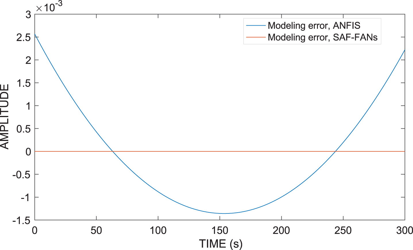
The mean squared error for ANFIS is J (300) = 6.3584e - 7 and for SAF-FAN is J (300) = 1.0313e - 25, Fig. 2.

Applying the fuzzy ANFIS and SAF-FAN methods, with error correction learning algorithms, very good results were obtained Figs. 3, 4, in addition to stable modeling, optimization of the system identification was achieved.

Fig. 4

Model 1, mean squared error of ANFIS and SAF-FANs.

5.2 Model 2. Nonlinear System Identification

A nonlinear system is used to illustrate the performance of RBF-NN, SAF-FAN, ANFIS and learning algorithm FANs (5-7, 12-14). A comparison is made between these methods. Equation (34), describes the identified plant [10], $\begin{matrix} y (k) = \frac{y (k - 1) \cdot y (k - 2) \cdot [y (k - 1) + 2.5]}{1 + y {(k - 1)}^{2} + y {(k - 2)}^{2}} \\ + u (k - 1) \end{matrix}$ (61)

5.2.1 SAF-FANs method

For this unknown nonlinear system (35), we propose the following standard form, $\begin{matrix} \hat{y} (k) = w_{in 11} \cdot (\hat{y} (k - 1) + w_{in 21}) + w_{in 31} \cdot \\ \hat{y} (k - 2) + w_{in 41} \cdot u (k - 1)) \cdot w_{in 51} \cdot g_{1} \end{matrix}$ (62)

Where g₁ = 3, u (k) are random numbers in [0,1]; we use the SAF-FANs for modeling the nonlinear plant, Figs. 5, 7.

Fig. 5

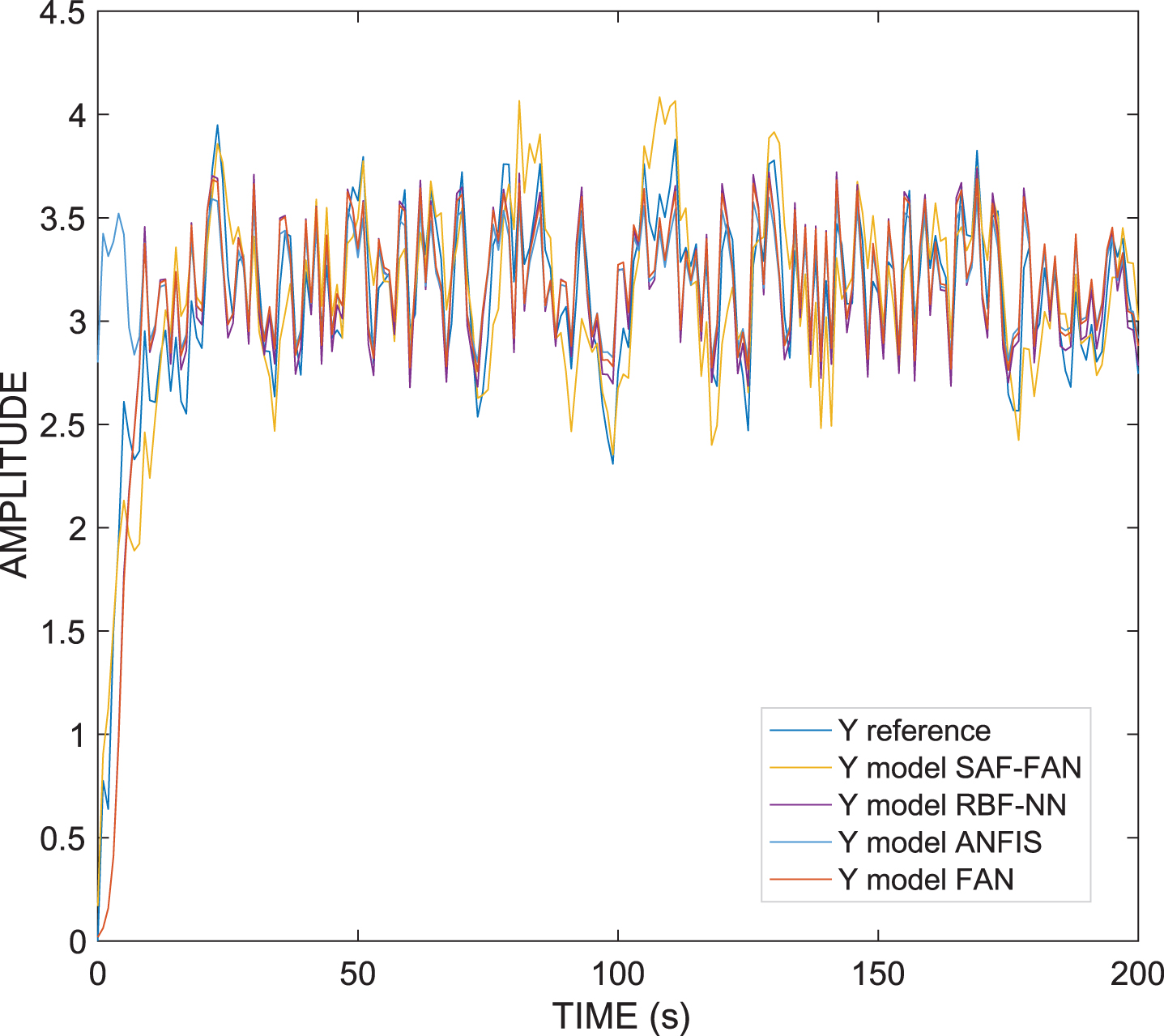
Model 2, Nonlinear System Identification in training based on SAF-FANs, RBF-NNs, ANFIS and Learning Algorithm FANs.

Fig. 6

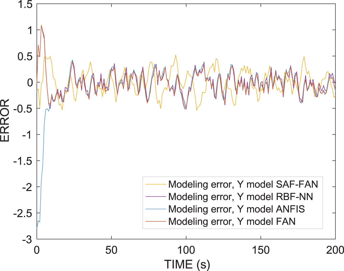
Model 2, mean squared error in training of SAF-FANs, RBF-NNs, ANFIS and Learning Algorithm FANs.

Fig. 7

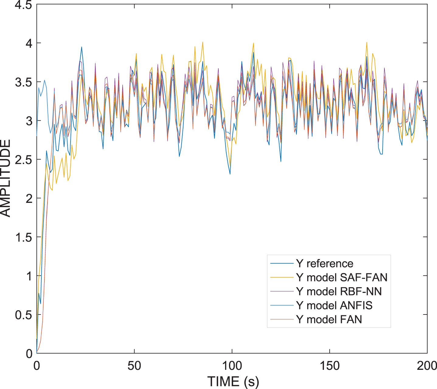
Model 2, Nonlinear System Identification with fixed parameters based on SAF-FANs, RBF-NNs, ANFIS and Learning Algorithm FANs.

For weight training, the error was normalized with a factor g₄ $e (k) = (y (k) - \hat{y} (k)) \cdot g_{2}$ , where g₂ = 0.01.

The error after training is defined for finite time as, $e (k) = y (k) - \hat{y} (k)$ (63)

Fixed weights were obtained after ten periods of training. J₁ (200) = 0.0276, Figs. 6, 8. The initial conditions,

Weights, w_{in FAN_ij} (k) =1; i = 1, ⋯ , 5; j = 1.

Learning factors, fixed values, γ_FAN i (k) =1.

The threshold values for all the FANs are, $V_{threshold 1 {FAN}_{i}} (k) = α_{A {FN}_{i}}^{-} = 0 .$

The values for the parameters a, b are,

a = 11, b = 2.

FANs inputs, z_{in FAN_i1} (k) =1.

Reference outputs ${\tilde{y}}_{refi} (k) = y (k)$ .

Ideal values of the weights are unknown.

Sampling period is K_sample = 1 second.

5.2.2 RBF-NNs method

For this unknown nonlinear system (36), we propose the following standard form, $\begin{matrix} \hat{y} (k) = (w_{in RBF 11} \cdot μ_{RBF 1} (k) + w_{in RBF 21} \cdot \\ μ_{RBF 2} (k) + u (k - 1)) \cdot \frac{1}{1 + e^{- k + c_{1}}} \end{matrix}$ (64)

Where u (k) are random numbers in [0,1], c₁ = 5; we use the RBF-NNs with error correction algorithm for modeling the nonlinear plant, Figs. 5, 7.

Fixed weights were obtained after ten periods of training. J₂ (200) = 0.0277, Figs. 6, 8. The initial conditions,

Weights, w_{in RBF_ij} (k) =0; i = 1, ⋯ , 2; j = 1.

Learning factors, fixed values, γ_FANi (k) =1.

δ_{RBF
_i} (k) =0, σ_{RBF
_i} (k) =0.0001.

RBFs inputs, z_{in RBF₁₁} (k) = u (k - 1) , $z_{in {RBF}_{21}} (k) = \hat{y} (k - 2)$ .

Reference outputs ${\tilde{y}}_{refi} (k) = y (k)$ .

Ideal values of the weights are unknown.

Sampling period is K_sample = 1 second.

5.2.3 ANFIS method

For this unknown nonlinear system, from (19), (37), we propose the following standard form, $\begin{matrix} \hat{y} (k) = φ (k) \cdot (w_{in 11} \cdot z_{in {ANFIS}_{11}} (k) + w_{in 21} \cdot \\ z_{in {ANFIS}_{21}} (k) + w_{in 31} \cdot z_{in {ANFIS}_{31}} (k) + w_{in 41} \cdot \\ z_{in {ANFIS}_{41}} (k) + w_{in 51} \cdot z_{in {ANFIS}_{51}} (k) + g_{3}) \cdot g_{4} \end{matrix}$ (65)

Where u (k) are random numbers in [0,1], g₃ = 0.035, g₄ = 4, we use ANFIS with error correction algorithm for fuzzy systems [10], for modeling the nonlinear plant, Figs. 5, 7.

Fixed weights were obtained after 20 periods of training. J₃ (200) =9.1525e - 4, Figs. 6, 8. The initial conditions,

Weights, w_{in ANFIS_ij} (k) =1; i = 1, ⋯ , 5; j = 1.

Learning factors, fixed values, η_ANFISi (k) =1.

Gaussian membership functions c_{ANFIS
_i} (k) =0.00001, σ_{ANFIS
_i} (k) =37e3.

ANFIS inputs, $z_{in {ANFIS}_{11}} (k) = \hat{y} {(k - 1)}^{2}$ $* \hat{y} (k - 2), z_{in {ANFIS}_{21}}$ $(k) = \hat{y} (k - 1) * \hat{y} (k - 2)$ , $z_{in {ANFIS}_{31}} (k) = \hat{y} {(k - 1)}^{2}$ , $z_{in {ANFIS}_{41}} (k) = \hat{y}$ (k - 2) ², z_{in ANFIS₅₁} (k) = u (k - 1).

Reference outputs ${\tilde{y}}_{refi} (k) = y (k)$ .

Ideal values of the weights are unknown.

Sampling period is K_sample = 1 second.

Fig. 8

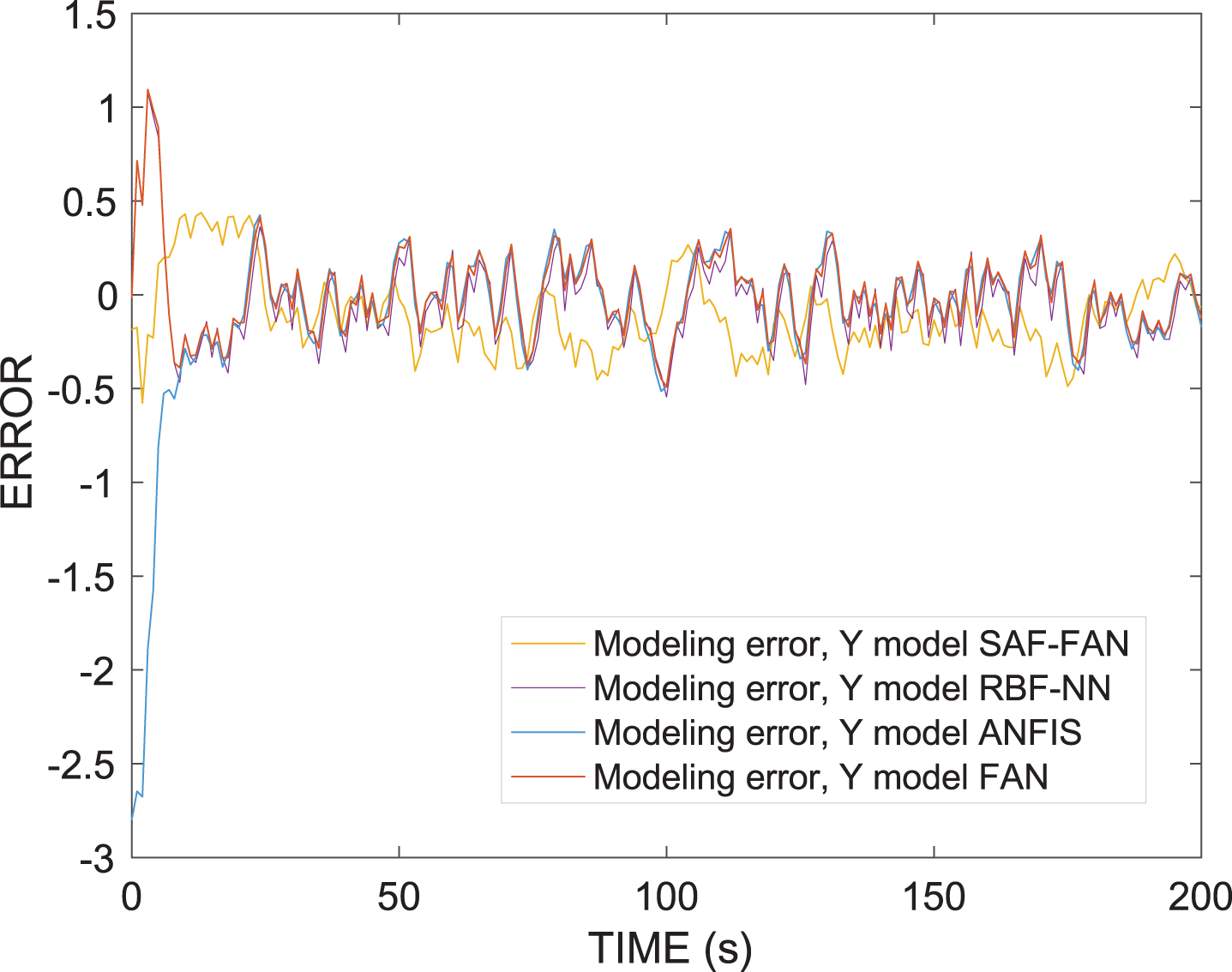
Model 2, mean squared error with fixed parameters of SAF-FANs, RBF-NNs, ANFIS and Learning Algorithm FANs.

5.2.4 FANs method

For this unknown nonlinear system (38), we propose the following standard form, $\begin{matrix} \hat{y} (k) = (w_{in 11} \cdot (w_{in 21} \cdot z_{in FAN 21} (k) + w_{in 31} \cdot \\ z_{in FAN 31} (k) + w_{in 41} \cdot z_{in FAN 41} (k) + w_{in 51} \cdot \\ z_{in FAN 51} (k)) + z_{in FAN 61} (k) + w_{in 61} - g_{5} \cdot \\ (w_{in 71} \cdot (w_{in 81} \cdot z_{in FAN 81} (k) + w_{in 91} \cdot \\ z_{in FAN 91} (k) + w_{in 101} \cdot z_{in FAN 101} (k) + w_{in 111} \cdot \\ z_{in FAN 111} (k)) + z_{in FAN 121} (k) \cdot g_{6} \cdot + w_{in 121}) + \end{matrix}$ $\begin{matrix} g_{7} \cdot (w_{in 131} \cdot (w_{in 141} \cdot z_{in FAN 141} (k) + w_{in 151} \cdot \\ z_{in FAN 151} (k) + w_{in 161} \cdot z_{in FAN 161} (k) + w_{in 171} \cdot \\ z_{in FAN 171} (k)) + z_{in FAN 181} (k) \cdot g_{8} + w_{in 181})) \cdot g_{9} \cdot \\ \frac{1}{1 + e^{- k + c_{1}}} \end{matrix}$ (66)

Where g₅ = 0.5, g₆ = 0.145, g₇ = 0.004, g₈ = 0.145, g₉ = 0.980075, c₁ = 5, u (k) are random numbers in [0,1]; we use the learning algorithm FANs for modeling the nonlinear plant, Figs. 5, 7.

The error after training is defined for finite time, $e (k) = y (k) - \hat{y} (k)$ (67)

Fixed weights were obtained after 20 periods of training. J₄ (200) = 2.6010e - 4, Figs. 6, 8. The initial conditions,

Weights, w_{in FAN_ij} (k) =1; i = 1, ⋯ , 18; j = 1.

Learning factors, fixed values, γ_FANi (k) =1.

Learning algorithm FANs inputs, z_{in FAN₁₁} (k) = z_{in FAN₂₁} (k) = z_{in FAN₇₁} (k) = z_{in FAN₈₁} (k) = z_{in FAN₁₃₁} (k) = z_{in FAN₁₄₁} $(k) = \hat{y} (k - 2), z_{in {FAN}_{31}} (k) = z_{in {FAN}_{91}}$ (k) = z_{in FAN₁₅₁} (k) = u (k - 1) , z_{in FAN₄₁} (k) = z_{in FAN₁₀₁} (k) = z_{in FAN₁₆₁} $(k) = \hat{y} (k - 1) z_{in {FAN}_{51}} (k) = z_{in {FAN}_{111}}$ $(k) = z_{in {FAN}_{171}} (k) = \hat{y} (k - 2)$ , z_{in FAN₆₁} (k) = z_{in FAN₁₂₁} (k) = z_{in FAN₁₈₁} (k) = u (k - 1).

Reference outputs ${\tilde{y}}_{refi} (k) = y (k)$ .

Ideal values of the weights are unknown.

Sampling period is K_sample = 1 second.

The results obtained from the simulation of model 1 of the two-dimensional function approximation Fig. 3, based on FAN, were considerably better compared to ANFIS.

The mean squared errors for models 1 and 2 are shown in Tables 1 and 2.

Table 1

Model 1, mean squared errors (MSE), J₁ (300), Figs. 3, 4

Method	MSE
ANFIS	6.3584e –7
SAF-FAN	1.0313e –25

Table 2

Model 2, mean squared errors (MSE), J₂ (200), Figs. 5–8

Method	MSE
	Training	Testing
SAF-FAN	0.0267	0.0276
RBF-NN	0.02430	0.0277
ANFIS	9.1522e –4	9.1525e –4
FAN	2.6737e –4	2.6010e –4

For model 2, the identification of the nonlinear system was carried out by four methods, SAF-FANs, RBF-NN, ANFIS and learning algorithm FAN. Comparing the results obtained from the simulations, Figs. 5-8, the mean squared errors of the FANs method in training and testing are much lower than those obtained with the RBF-NN and ANFIS methods, Fig. 8.

FANs, based on the results of simulations of models 1-2, have identified the proposed nonlinear systems with great precision, showing their potential for systems modeling.

6 Conclusion

For the identification of nonlinear systems, in this article, we solve the problem with the FANs learning algorithm and SAF. Stability analysis was performed successfully in Section 4.

The results obtained from the modeling simulation of the nonlinear systems in Section 5 show that the identification of systems with FAN is performed more efficiently than other methods such as RBF-NN and ANFIS. Reducing the error considerably, through configurations of FANs and SAF.

Multiple applications can be carried out applying the FANs method, with their learning algorithm for fuzzy systems, and activation functions SAF, for systems identification, control and automation of systems, low-scale unmanned aerial vehicles (UAVs), optimization of manufacturing processes by laser beam, seismic systems to model their behavior by processing seismic accelerograms, image processing among others [23 , 32–34].

Footnotes

Acknowledgment

We would like to thank the support of the CONACYT Postdoctoral Scholarship Program, together with the Department of Automatic Control and Computer Department of CINVESTAV-IPN, CONACYT Research Fellows -CIIIA, FIME, UANL Program and Electromechanical Engineering Division, ITSOEH.

References

Widrow

and Lehr

M.A.

, 30 Years of adaptive neural networks: perceptron, madaline, and backpropagation, Proceedings of the IEEE 78(9) (1990), 1415–1442.

Werbos

P.J.

, The Roots of Backpropagation From Ordered Derivatives to Neural Networks and Political Forecasting. Wiley Series on Adaptive and Learning Systems for Signal Processing, Communications, and Control. Ed. John Wiley & Sons, Inc. Wiley-Interscience (1994), 320 p., ISBN 0-471-59897-6

Gupta

M.M.

and Qi

, On Fuzzy Neuron Models. Fuzzy logic for the management of uncertainty, In Lotfi A. Zadeh et al (Eds.), Wiley-Interscience (1992), 479–491. ISBN: 0-471-54799-9

Gupta

M.M.

, Fuzzy logic, neural networks and virtual cognitive systems, In Second International Symposium on Uncertainty Modeling and Analysis, IEEE (1993), 90–97. DOI. 10.1109/ISUMA.1993.366785

Gupta

M.M.

and Rao

D.H.

, On the principles of fuzzy neural networks, Fuzzy Set Syst, Elsevier Science B. V. 61 (1994), 1–18.

Rubio

J.J.

and Yu

, Stability analysis of nonlinear system identification via delayed neural networks, IEEE T. Circuits-II 54(2) (2007), 161–165. DOI: 10.1109/TCSII.2006.886464

Ramírez-Mendoza

, Covarrubias-Fabela

, Amezquita-Brooks

and Hernández-Alcantara

, Parameter Identification using Fuzzy Neurons: Application to Drones and Induction Motors, DYNA-Bilbao 93(1) (2018a), 75–81. DOI: https://dx-doi-org.web.bisu.edu.cn/10.6036/8439

Ramírez-Mendoza

A.M.E.

, Modeling the Spike Response for Adaptive Fuzzy Spiking Neurons with Application to a Fuzzy XOR, Tech Science Press 115(3) (2018b), 295–311. DOI. 10.3970/cmes.2018.00239 [Printed] ISSN:1526-1492 [Online] ISSN:1526-1506

Zadeh

L.A.

, Theory of Fuzzy Sets, Encyclopedia of Computer Science and Technology, Marcel Dekker, Nueva York, E.U.A, 1977).

10.

and Li

, Fuzzy identification using fuzzy neural networks with stable learning algorithms, IEEE T. Fuzzy Syst. 12(3) (2004), 411–420. DOI: 10.1109/TFUZZ.2004.825067

11.

and Rubio

J.J.

, Recurrent neural networks training with stable bounding ellipsoid algorithm, IEEE Transactions on Neural Networks 20(6) (2009), 983–991. DOI: 10.1109/TNN.2009.2015079

12.

Z.J.

, Xie

W.F.

, Han

and Luo

W.D.

, Nonlinear systems identification and control via dynamic multitime scales neural networks, IEEE Neur. Net. Lear. 24(11) (2013), 1814–1823.

13.

Han

, Wu

, Liu

and Qiao

, Data-knowledge-based fuzzy neural network for nonlinear system identification, IEEE Fuzzy Syst., DOI 10.1109/TFUZZ.2019.2931870

14.

Cervantes

, Yu

, Salazar

and Chairez

, Takagi–Sugeno dynamic neuro-fuzzy controller of uncertain nonlinear systems, IEEE T. Fuzzy Syst 25(6) (2017), 1601–1615. DOI: 10.1109/TFUZZ.2016.2612697

15.

Dubois

and Prade

, Towards fuzzy differential calculus. Part 1: Integration of fuzzy mappings, North-Holland Publishing Company 8 (1982), 1–17.

16.

Pérez

J.L.

and Ramírez

, Two new models of integrative fuzzy neuron, Instrumentation & Development 5(3) (2001), 140–145.

17.

Ramírez

and Pérez

J.L.

, A Fuzzy Gupta Integrator Neuron Model with Spikes Response and Axonal delay, In Advances in Artificial Intelligence &Engineering Cybernetics, IX; Windsor. Canada: IIAS. In George E. Lasker (Ed.) (2002), 12–16. ISBN: 1-894613-44-9

18.

Ramírez-Mendoza

, Pérez-Silva

J.L.

and Lara-Rosano

, Electronic implementation of a fuzzy neuron model with a gupta integrator, JART-Journal of Applied Research and Technology 9(3) (2011), 380–393. ISSN: 1665-6423, [Online]. Available: http://cibernetica.ccadet.unam.mx/jart/vol9_3/electronic_10.pdf

19.

Ramírez-Mendoza

, Study of the response of the connection of Adaptive Fuzzy Spiking Neurons with self-synapse in each single neuron, 11th International Conference on Electrical Engineering, Computing Science and Automatic Control (CCE), Ciudad del Carmen, Campeche, México (2014), 1-6. ISBN: 978-1-4799- 6228-0.

20.

Ramírez-Mendoza

A.M.E.

, Design of a PID controller based on Adaptive Fuzzy Spiking Neurons, Memories of the National Congress of Automatic Control (CNCA), San Luis Potosí, México, 10-12 October, (2018c), ISSN 2594-2492.

21.

Ramírez-Mendoza

A.M.E.

and Yu

, A novel learning algorithm for Adaptive Fuzzy Neural Networks: Application to the neuro-fuzzy design of control law for a PID controller. Soft Comput (under review a).

22.

Ramírez-Mendoza

A.M.E.

, Covarrubias-Fabela

J. R.

, Amezquita-Brooks

L. A.

, García-Salazar

, Yu

, Fuzzy Adaptive Neurons Applied to the Identification of Parameters and Trajectory Tracking Control of a Multi-Rotor Unmanned Aerial Vehicle Based on Experimental Aerodynamic Data, J. Intell. Robot Syst. (2020), 1–19. ISSN: 0921-0296. DOI. 10.1007/s10846-020-01198-w.

23.

Ramírez-Mendoza

A.M.E.

, Yu

and Li

, A Novel Fuzzy System with Adaptive Neurons for Earthquake Modeling, IEEE Access, 8(1) (2020), 101369–101376, Print ISSN: 2169-3536, Online ISSN: 2169-3536, DOI. 10.1109/ACCESS.2020.2998446

24.

Ramírez-Mendoza

A.M.E.

, Yu

and Li

, A new spike membership function for the recognition and processing of spatiotemporal spike patterns: syllable-based speech recognition application. Fuzzy Set Syst (under review b).

25.

Zhao

and Bose

B.K.

, Evaluation of membership functions for fuzzy logic controlled induction motor drive, IEEE (2002), 229–234. 0-7803-7474-6/02

26.

Mazandarani

and Li

, Fractional fuzzy inference system: The new generation of fuzzy inference systems, Access 8 (2020), 126066–126082. DOI: 10.1109/ACCESS.2020.3008064

27.

Vatankhah

, Ghanatian

and Kahraman Cengiz

, Artificial neural networks and adaptive neuro-fuzzy inference systems for parameter identification of dynamic systems, Journal of Intelligent & Fuzzy Systems 39(5) (2020), 6145–6155. DOI: 10.3233/JIFS-189085

28.

Khalil

H.K.

, Nonlinear Systems, Ed. Prentice Hall; (2002), 750 p. ISBN: 0-13-067389-7.

29.

Sanchez

E.N.

and Ornelas-Tellez

, Discrete-Time Inverse Optimal Control for Nonlinear Systems, Ed. Prentice Hall, (2002), 750 p. ISBN: 0-13-067389-7.

30.

Dong

, Bao

, Zheng

, Yang

, Song

and Mao

, Heading control of unmanned marine vehicles based on an improved robust adaptive fuzzy neural network control algorithm, IEEE Access 7 (2019), 9704–9713. DOI: 10.1109/ACCESS.2019.2891106

31.

Mandic

D.P.

, Hanna

A.I.

and Razaz

, A normalized gradient descent algorithm for nonlinear adaptive filters using a gradient adaptive step size, IEEE Signal Processing Lett. 8 (2001), 295–297.

32.

Gerstner

and Kistler

W.M.

, Spiking Neuron Models, Ed. Cambridge University Press, (2002), 480 p. ISBN: 978-0521890793.

33.

Susi

, Toro

L.A.

, Canuet

, López

M.E.

, Maestú

, Mirasso

C.R.

and Pereda

E.A.

, Neuro-Inspired System for Online Learning and Recognition of Parallel Spike Trains, Based on Spike Latency, and Heterosynaptic STDP, Front Neurosci-Switz 12(780) (2018), 1–14. DOI: 10.3389/fnins.2018.00780

34.

Amezquita-Brooks

L.A.

, Hernández Alcántara

, Santana-Delgado

, Covarrubias-Fabela

J.R.

, García-Salazar

and Ramírez-Mendoza

A.M.E.

, Improved model for micro-UAV propulsion systems: characterization and applications, IEEE T AERO ELEC SYS. 56(3) (2020), 2174–2197. Print ISSN: 0018-9251, Online ISSN: 1557-9603. DOI. 10.1109/TAES.2019.2943756