Multi-gene genetic programming to building up fuzzy rule-base in Neo-Fuzzy-Neuron networks

Abstract

This paper introduces a new approach to build the rule-base on Neo-Fuzzy-Neuron (NFN) Networks. The NFN is a Neuro-Fuzzy network composed by a set of n decoupled zero-order Takagi-Sugeno models, one for each input variable, each one containing m rules. Employing Multi-Gene Genetic Programming (MG-GP) to create and adjust Gaussian membership functions and a Gradient-based method to update the network parameters, the proposed model is dubbed NFN-MG-GP. In the proposed model, each individual of MG-GP represents a complete rule-base of NFN. The rule-base is adjusted by genetic operators (Crossover, Reproduction, Mutation), and the consequent parameters are updated by a predetermined number of Gradient method epochs, every generation. The algorithm uses Elitism to ensure that the best rule-base is not lost between generations. The performance of the NFN-MG-GP is evaluated using instances of time series forecasting and non-linear system identification problems. Computational experiments and comparisons against state-of-the-art alternative models show that the proposed algorithms are efficient and competitive. Furthermore, experimental results show that it is possible to obtain models with good accuracy applying Multi-Gene Genetic Programming to construct the rule-base on NFN Networks.

Keywords

Neo-fuzzy-neuron genetic programming multi-gene NFN-MG-GP forecasting non-linear system identification

1 Introduction

Neuro-Fuzzy networks are Computational Intelligence techniques that combine characteristics of the Fuzzy Systems and Neural Networks. These systems stand out for integrating the treatment of uncertainty and the interpretability of Fuzzy Systems and the learning ability provided by Neural Networks [40]. Neuro-Fuzzy networks present benefits over other Artificial Intelligence (AI) techniques since they have high learning and generalization capacity and can be explainable - meaning that it is possible to explain why the training method reaches a determined solution [3, 34]. On the other hand, Fuzzy Systems lack learning and generalization capabilities, and Neural Networks are not explainable [34].

From the 90s, many works have improved Neuro-Fuzzy Systems and achieved great results. Neuro-Fuzzy systems have become highly efficient due to its fast learning, on-line adaptability, self-adjusting, the capability of obtaining the small global error possible, and small computational complexity [47]. Furthermore, the capacity of obtaining good results is one of the responsible for them to be considered universal approximators [27 , 57].

Neuro-Fuzzy networks have been applied in different domains such as forecasting [2], non-linear systems identification [15], classification [7, 29], control systems [42], among others. Some works have already made a comparison between Neuro-Fuzzy networks and other AI techniques. For example, [16] compares Multi-Gene Genetic Programming (MGGP) and a dynamic evolving neural-fuzzy inference system (DENFIS) to modeling pan evaporation, showing some advantages of DENFIS to prediction and MGGP to regression in data. In [44] Neuro-Fuzzy and Neuro-Bee models for predicting the safety factor of eco-protection slopes are evaluated, obtaining a high prediction capacity in the Neuro-Fuzzy model. Some AI tools, including Genetic Programming (GP) and Adaptive Neuro-Fuzzy Inference System (ANFIS), are evolved to determinate relationships between groundwater quality parameters in [4]. ANFIS has demonstrated efficiency to estimate these parameters and GP to model the relationships.

There is a growing interest in developing new learning algorithms that enable the autonomous construction of the rule-base and parameters’ update in Neuro-Fuzzy networks using Machine Learning techniques [47]. Among the approaches used for learning in Neuro-Fuzzy networks are Evolutionary Computation techniques that stand out for their ability to adapt and learn, based on a global search [20].

Evolutionary Computation algorithms can be used to extract knowledge to the construction of the rule-base [26] and to parameters’ update [24]. There are two main approaches to creating rules with Evolutionary Computation techniques, that of Michigan [21] and that of Pittsburg [50]. Michigan’s approach defines that each individual represents one rule, and the rule-base is a set of individuals. In this case, the individual’s modeling is simpler, but its evaluation becomes harder due to the need to define a rule’s quality. In the Pittsburg approach, each individual encodes a set of rules, thus facilitating their assessment, since a single individual represents the entire rule-base. On the other hand, computational cost and training time become higher when compared to the other approach.

Evolutionary methods, population-based algorithms inspired by biological evolution principles, distinguish from other heuristic methods mainly by their ability to avoid local optimal [17]. Being populational methods, they can converge in fewer steps than others. Specifically, Genetic Programming (GP) has already been demonstrated to be efficient when applied to regression problems due to its high capability of representing complete functions [6, 38]. Such as discussed in [47], a single supervised learning technique, such as gradient-based technique, suffers from local minima and overfitting problems. Furthermore, a single technique can be exhaustive and present weak firing strength when the network structure and parameters become large [33, 46]. Instead, population-based algorithms are derivative-free algorithms and do not require the differentiability assumption. Those algorithms require only the availability of objective function values but no derivative information. It is particularly useful when the derivative of the function is difficult to obtain or does not exist.

This work introduces an evolutionary Neuro-Fuzzy system that hybridizes the neurocomputing approach with the searching ability of the evolutionary techniques. Here, an algorithm based on Multi-Gene Genetic Programming (MG-GP) to build the rule-base of a Neo-Fuzzy-Neuron (NFN) network [55] using the Pittsburg approach is proposed. Since in the Pittsburgh approach, an entire fuzzy rule base is encoded as a chromosome, when applying the Genetic Programming, an individual of the population represents a complete rule-base. The MG-GP creates and adjusts the membership functions, and a Gradient-based method adjusts the network’s parameters. Although much explored in Fuzzy and Neuro-Fuzzy Systems and shown to be efficient methods to learning in these systems, Evolutionary Algorithms, in particular Genetic Programming, are still unexplored in NFN networks. The novelties and the main contributions presented in this work are:

Integration of Multi-Gene-Genetic-Programming and Gradient-based Method to automatic generation and adjustment of rules and parameters in Neo-Fuzzy-Neuron networks;

The Neo-Fuzzy-Neuron models are evolved in the evolutionary learning processes;

A new learning algorithm to Neo-Fuzzy-Neuron Networks focused on solving general regression problems;

Obtaining a Neuro-Fuzzy System based on data with good accuracy.

Genetic Programming, a class of evolutionary approaches, encodes data in the genetic individuals, and the search is performed on this coding instead of raw data. This feature allows GP to be independent of the continuity of the data [47]. The rationale behind the choice of hybrid algorithm, coupling Multi-Gene Genetic Programming and Pittsburg approach, is based on the following:

Genetic Programming can be seen as an extension of popular Genetic Algorithms combining their global search ability and their renowned efficiency.

In Genetic Programming, one individual is modeled as a complete rule base in a tree-like arranged nodes. Since the fuzzy sets are encoded into the genotype, it facilitates evaluating solutions and fuzzy rules. It allows the generation of more suited fuzzy sets to describe membership functions via the intersection and/or union of the existing fuzzy sets.

Every component of the resulting rule-base is relevant in some way for the problem’s solution. Therefore, the GP does not encode null operations that will expend computational resources at runtime.

The proposed approach does not scale up with the problem size, differently from other approaches that work poorly when the problem grows in size. This would be the case when using a Genetic Algorithm to encode an N × N matrix. It is important to notice that, using Genetic Programming, any restriction on the structure of solutions is imposed. Besides, nor the complexity neither the number of rules of the solution is bounded.

The aspects discussed above give significant advantages to Genetic Programming in Neuro-Fuzzy Systems’ learning processes [5] over other heuristic and populational methods such as ACO [43], PSO [37], ABC [14], among others.

After this brief introduction, the remainder of this paper is organized as follows. Section 2 presents a short review of works that used evolutionary computation techniques to learning in Neuro-Fuzzy networks and other techniques used to learning in NFN. Section 3 describes the Neo-Fuzzy-Neuron (NFN) network and addresses its learning algorithm. Section 4 presents the proposed approach, the Neo-Fuzzy-Neuron with the Multi-Gene Genetic Programming (NFN-MG-GP). Section 5 details the computational experiments and discusses the results. Finally, Section 6 concludes the paper with a summary of its contributions and suggestions for further studies.

2 Related works

The synergy of Fuzzy Systems and Evolutionary Computation has been extensively explored since the 90s, aiming to integrate the management of uncertainty and the interpretability of Fuzzy Systems with the learning and adaptability of Evolutionary Computation [17]. Several works explored Evolutionary Computation for learning in Fuzzy Systems and Neuro-Fuzzy networks. Most of these works applied Genetic Algorithms (GA), but there are also approaches utilizing other techniques like Genetic Programming (GP).

Using GP, [26] presents a Fuzzy System for classification. The work uses Multi-Gene Genetic Programming to create and adjust the rule-base of a Pittsburg Genetic Fuzzy System. In [35], a multi-tree GP model is used to improve the accuracy of a Takagi-Sugeno Fuzzy System for dynamic portfolio mapping.

A Genetic Neuro-Fuzzy Inference Method (GENFIS) for diagnosis of Tuberculosis is presented in [39]. The GA was used to select the ideal network input parameters, which are used for diagnosis. The work of [5] presents an approach that uses Neuro-Fuzzy models to identify the main factors responsible for depression. In addition to optimizing weights, the AG, fleeing from great locations, also made it possible to identify redundant and inexpressive rules, thus obtaining a cleaner and more optimized rule-base. In [51], a Neuro-Fuzzy Hybrid System called ANFIS-GA (Adaptive Neuro-Fuzzy Inference System with Genetic Algorithm) is introduced. In ANFIS-GA, the GA is used to adapt the parameters of an ANFIS network. In this work, the antecedent and consequent of the fuzzy rules are modeled as GA variables.

The work of [19] presents a Genetic Neuro-Fuzzy Systems to detect faulty bearings. GA determines the adequate values to parameters to achieve a reduced number of nodes on the hidden layer. Each individual represents one structure of hidden nodes. [1] proposed an Adaptative Neuro-Fuzzy Inference System (ANFIS) trained by GA to Forecasting crude oil price. The ANFIS parameters are adjusted by GA, defining the best weights between layers 4 and 5 are optimized by GA.

However, the use of evolutionary techniques in NFN-type networks is still underexplored. In Neo-Fuzzy-Neuron networks, most works use methods based on Gradient and least-squares. In [13], an extended NFN network is proposed with adaptive learning by Backpropagation to adjust the network parameters. In this approach, the universe of discourse is uniformly partitioned by triangular and complementary functions. In [22], the authors use the same structure and present an architecture and methods for deep NFN networks with online parameters update using the weighted recurring least squares method with adaptive and cascading learning. The membership functions are triangular and complementary, created from uniform partitions.

A simple and automatic approach to design Neo-Fuzzy-Neuron networks for non-linear system identification is proposed by [32]. The network is composed of triangular and complementary functions created with the uniform partitioning of the universe of discourse. A least-squares with Backfitting obtains the network parameters. In [45], a convex cascade NFN network is proposed. The cascade architecture allows training each neuron cell independently and updates network parameters using a Gradient-based method. The membership functions used are complementary triangular and uniformly spaced.

An extended Neo-Fuzzy-Neuron structure is used in the work of [9], with unified pertinence functions of the type B-Spline [54]. A Gradient-based algorithm is used to adapt the network parameters. In [10], an NFN network powered by multidimensional non-linear weights is proposed. Weights are adjusted by a method based on Gradient with Backpropagation, and the learning rate is given by an optimal method of recurring least-squares (only one step). In [12] authors present a new algorithm to adaptive training rule for a hybrid cascade neural network based on an application of a specific type of NFN elements. The suggested model has a hybrid cascade structure, following the hybrid cascade neural network’s topology on the grounds of an optimized pool in each cascade, proposed by the same authors in previous works, combining elementary Rosenblatt perceptrons with neo-fuzzy neurons on a structural block. Besides that is presented a modified procedure by Kaczmarz–Widrow–Hoff [23] for training the system. Were used a combination of different membership function for each node, as triangular and B-splines.

[56] presents and investigates a hybrid self-organized model called GMDH-neo-fuzzy Neural Network with deep learning. The GMDH method is a self-organization method and allows the optimal structure to be built to a neo-fuzzy system and adjust the weights of the neural network in just one procedure. A hybrid model was suggested where a Neo-Fuzzy Network with a small number of adjustable parameters was utilized as a node of the GMDH-System. The NFN model utilized was the original model proposed by Yamakawa in [55]. The same structure was used in [11] applied to Forecasting Problems in Finacial Sphere. A difference to the previous model is that each node of the GMDH-system, representing by one Neo-Fuzzy Network, uses only two inputs. The approach aims to prevent deep learning drawbacks, such as vanishing or exploding of the gradient method. An accelerated backpropagation algorithm to a deep Neo-fuzzy Neural Network is described in [8]. The proposed network consists of a traditional multilayer feedforward architecture with a layer to information processing and a neo-fuzzy neuron network as a node. It was used triangular membership functions with non-linear synapses. The learning method presented to the model is based on an error backpropagation algorithm. The learning process is performed through the search of synaptic weight coefficients by minimization of the chosen loss function and uses a standard squared function as a learning criterion.

After this brief review is possible to see that evolutionary algorithms demonstrated an efficient and interesting method to perform the learning tasks in Fuzzy and Neuro-Fuzzy Systems. Despite its popularity in other contexts, they are still unexplored in the NFN networks domain.

3 Neo-Fuzzy-Neuron

This section reviews the Neo-Fuzzy-Neuron (NFN) network [55] used to implement the proposed algorithm presented in Section 4. Neo-Fuzzy-Neuron is a Neuro-Fuzzy network composed of a set of n zero-order Takagi-Sugeno (TS) models [52], one for each input variable. The NFN can be summarized in 4 steps. Initially, the firing degree of the membership functions μ_{A
_ij} is calculated for each i input variable, in which j indexes the membership functions and i the input variables. In the second step, for each input variable, the degree of activation of the membership functions is multiplied by its respective weight q_ij, thus obtaining an output for each rule. After each rule output, the output of each TS model (y_ti) can be obtained just by aggregation of all rules. The way to perform the aggregation of all rules is detailed later on. Finally, the network output is obtained by the aggregation of the output of each TS model. Figure 1 illustrates the basic structure of the NFN network, and each step is detailed as follows. In this figure, x_ti is the input variable i at time t, y_ti the zero-order TS model output, ${\hat{y}}_{t}$ the output of the network, μ_{A
_ij} is the activation degree of membership function j by the input variable x_ti, and q_ij is the parameter associated with membership function A_ij [48].

In NFN, each membership function with its respective weight q_ij represents one rule. The domain of each input variable x_ti is partitioned into m_i membership functions [49]. Thus, with the partition of the input variable domain i, we have the following m_i TS rules:

Fig. 1

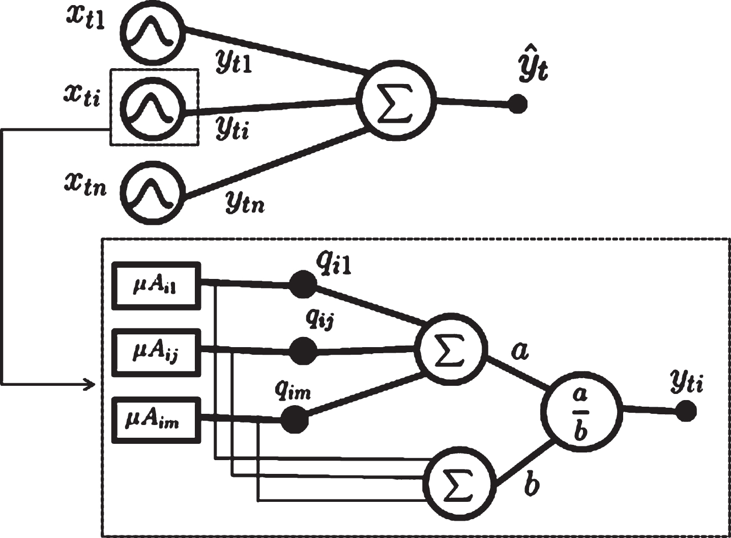
Neo-Fuzzy-Neuron network basic structure.

$\begin{matrix} R_{i}^{1} & If & x_{ti} is A_{i 1} & Then & y_{ti} is μ_{A_{i 1}} q_{i 1} \\ . . . \\ R_{i}^{j} & If & x_{ti} is A_{ij} & Then & y_{ti} is μ_{A_{ij}} q_{ij} \\ . . . \\ R_{i}^{m_{i}} & If & x_{ti} is A_{{im}_{i}} & Then & y_{ti} is μ_{A_{{im}_{i}}} q_{{im}_{i}} . \end{matrix}$

The models are decoupled, and the zero-order TS models output y_ti is obtained by Equation (1). In this way, the output y_ti is computed by the sum of the activation degree of each rule μ_{A
_ij} (x_i) multiplied by its respective parameter q_ij (a), weighted by the sum of the activation degree of all rules (b).

$\begin{matrix} y_{ti} = \frac{a}{b} = \frac{\sum_{j = 1}^{m_{i}} μ_{A_{ij}} (x_{i}) q_{ij}}{\sum_{j = 1}^{m_{i}} μ_{A_{ij}} (x_{i})}, \end{matrix}$ (1)

in which i indexes the input variables, j the membership functions, and t denotes the current step.

The NFN output in t ( ${\hat{y}}_{t}$ ) is computed by the sum of n zero-order TS models output y_ti using: ${\hat{y}}_{t} = \sum_{i = 1}^{n} y_{ti} .$ (2)

3.1 Membership functions

Although the membership functions used in the NFN proposed by [55] are Triangular, other membership functions can also be used, such as Gaussian or Spline [12 , 56]. In this work, we use Gaussian functions because it is an adequate function to represent uncertain data [28]. A Gaussian membership function is represented by its center (c) and spread (s). The activation degree μ_{A
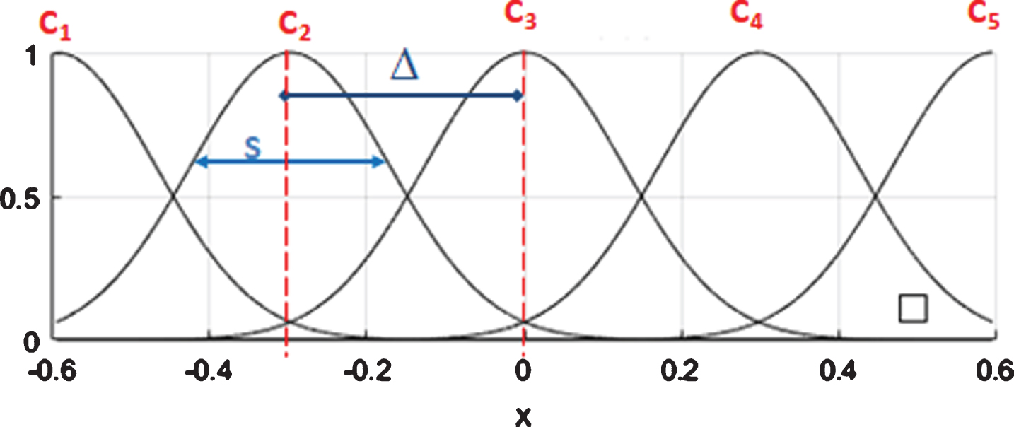
_ij} (x_ti) of a Gaussian membership function for a variable x_ti is given by Equation (3). Figure 2 ilustrates the structure of a Gaussian membership function. $\begin{matrix} μ_{A_{ij}} (x_{ti}) = \exp (- \frac{1}{2} (\frac{x_{ti} - c_{ij}}{s_{ij}})^{2}) . \end{matrix}$ (3)

Fig. 2

Uniformly Gaussian membership functions.

Gaussian membership functions can granulate the domain of input variable in two ways: uniformly spaced or non-uniformly spaced. Uniformly spaced membership functions consider that all rules cover the same range of values in the input variable’s domain. Figure 2 shows an example, in which the domain of the input variable is granulated into five uniformly spaced Gaussian membership functions. Note that the distance between the center of the functions (Δ) and the spread (s) are the same for all functions. Δ is given by Equation (4) and c is computed using Equation (5): $\begin{matrix} Δ_{i} = \frac{(\max_{x_{i}} - \min_{x_{i}})}{m_{i} - 1}, \end{matrix}$ (4)

$\begin{matrix} c_{ij} = \min_{x_{i}} + (j - 1) Δ_{i}, \end{matrix}$ (5)

in which i indexes the input variable, m_i is the number of membership functions for the variable i, j indexes the membership function, $\max_{x_{i}}$ is the upper bound of variable x_i, and $\min_{x_{i}}$ is the lower bound of variable x_i.

In non-uniformly spaced Gaussian membership functions, there is no definition of a single value for c or s. Thus, membership functions can be freely distributed throughout the universe of discourse, as shown in Fig. 3. Note that, in this case, there is no need to calculate Δ. Non-uniformly spaced functions can be considered generalized functions as they are more adaptable to the context of the problem to be solved [25]. Having that in mind, we opted to use non-uniformly spaced functions in this work.

Fig. 3

Non-uniformly Gaussian membership functions.

3.2 NFN parameters’ update

The procedure to update the network parameters is carried out using a Gradient-based method. The learning is supervised and aims updating q_ij [49]. The parameters q_ij are updated only for the active membership function according to Equation (6):

$q_{ij} = q_{ij} - α (y_{t} - {\hat{y}}_{t}) x_{ti} d_{ij},$ (6)

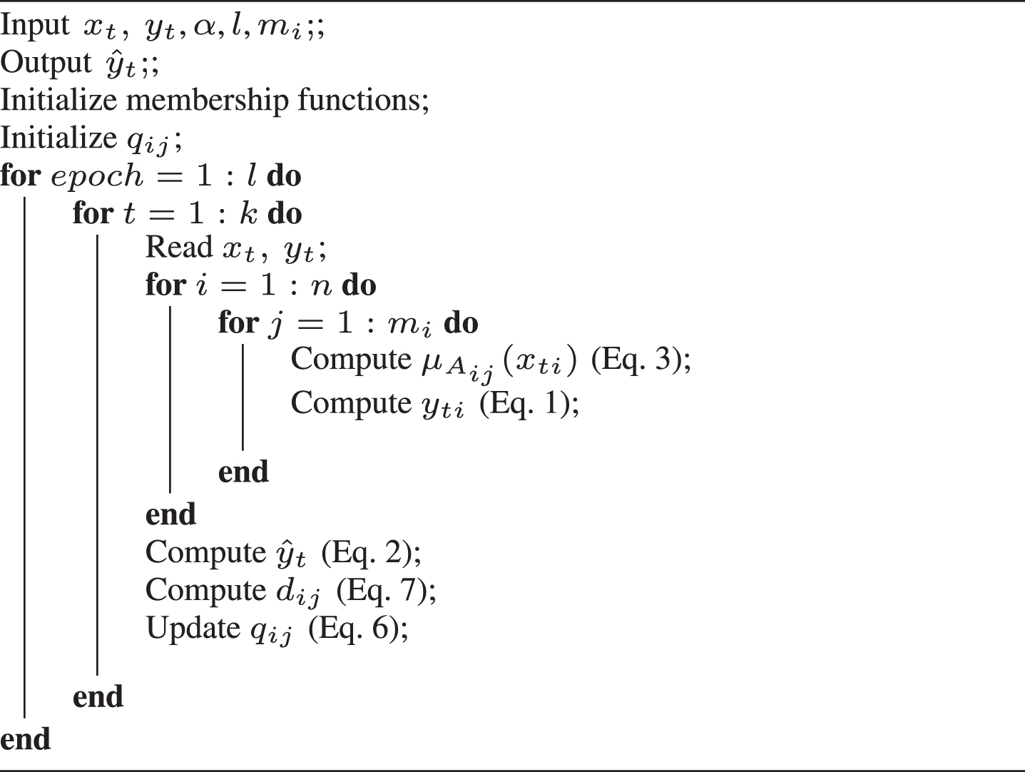
in which α is the learning rate, y_t is the desired output, ${\hat{y}}_{t}$ is the network ouput, and d_ij is obtained by:

$d_{ij} = \frac{μ_{A_{ij}}}{\sum_{j = 1}^{m_{i}} μ_{A_{ij}}} .$ (7)

The NFN parameters q_ij can be initialized randomly between 0 and 1. Algorithm 3.2 summarizes how to compute the output and update the parameters of the NFN network. In this algorithm, we use the number of epochs (l) as a stopping criterion for the training, but error measures such as RMSE and MSE can also be used.

Algorithm 1 NFN Algorithm.

4 NFN-MG-GP - Neo-Fuzzy-Neuron with multi-gene genetic programming

This section introduces the proposed approach to building up the Neo-Fuzzy Neuron network rule-base. The Pittsburg method [50], in which one individual represents a complete rule-base, is used with Multi-Gene Genetic Programming (MG-GP) [18] to create the NFN network rule-base and a Gradient-based method to adjust the parameters.

MG-GP is a variation of Genetic Programming (GP) considers that one individual has several trees connected by a linear structure of genes. The output of each individual is the aggregation of the trees linked to each superior gene. In NFN-MG-GP, each superior gene represents a zero-order TS model, and each one is associated with an arity tree m, in which m is the number of membership functions. A sub-tree linked to the central node represents a membership function, and the root node is composed of an aggregation function that returns the result of the membership functions associated with that model, as discussed in Section 3 and shown in Fig. 1. One individual of NFN-MG-GP is shown in Fig. 4.

Fig. 4

Example of individual on NFN-MG-GP.

The NFN-MG-GP seeks to find the best rule-base for NFN network using Multi-Gene Genetic Programming (MG-GP), which models possible rule-bases as individuals and adjusts its evolutionary process. Thus, each individual of MG-GP represents one rule-base to NFN. To ensure that the best rule-base is not lost between generations, the Elitism operator replicates the best individual to the next generation. The consequent parameters are created in the NFN module and updated by the Gradient Method. The set of parameters is the same for all individuals of Genetic Programming. Summarizing, the rule-base is adjusted by genetic operators (Crossover, Reproduction, Mutation, Elitism) at each GP generation. The consequent parameters are updated by the Gradient learning method. Figure 5 illustrates this process, highlighting the steps performed by the GP module and by the NFN module. Section 4.1 details the steps of the algorithm.

Fig. 5

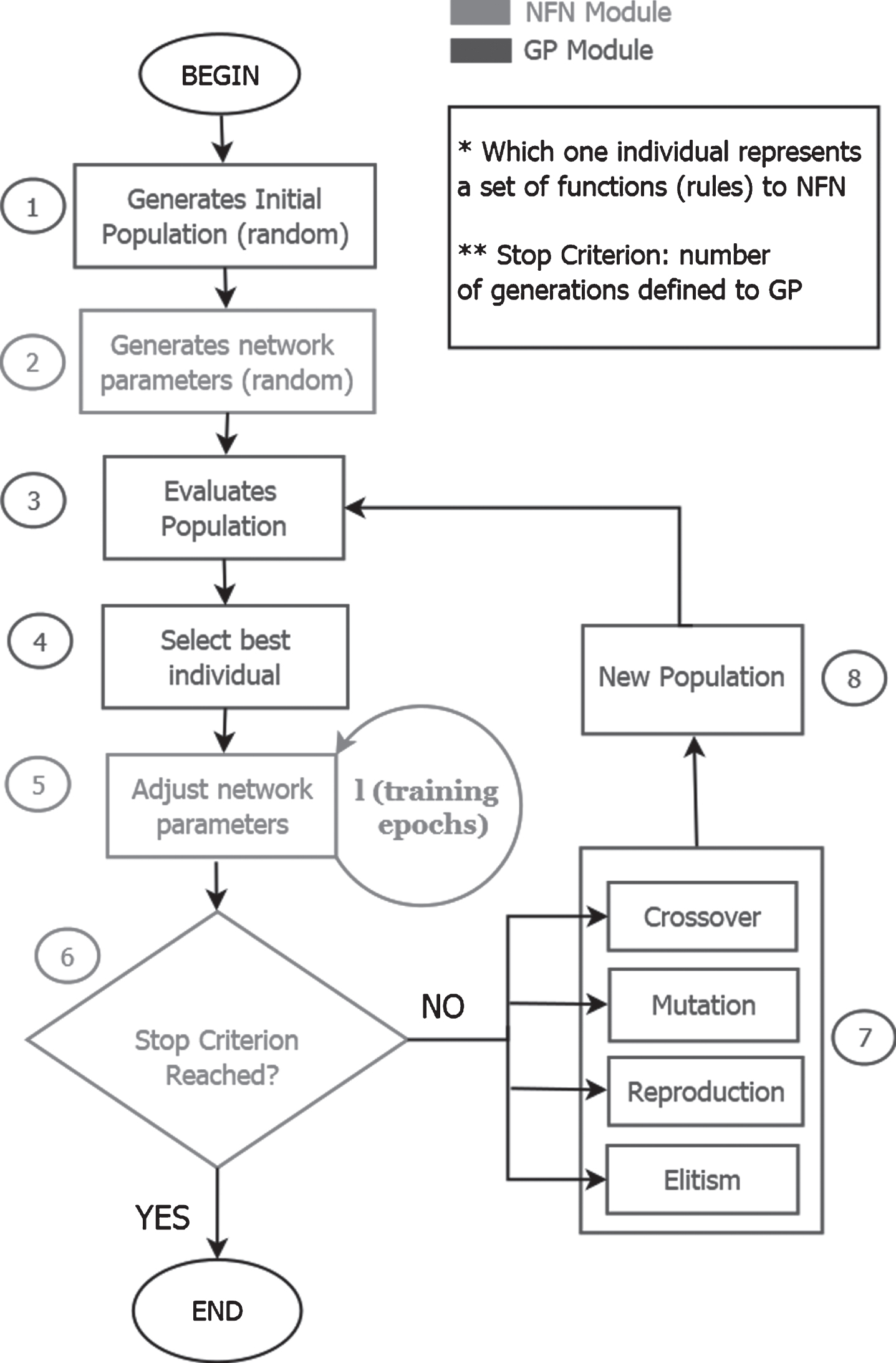
NFN-MG-GP algorithm flowchart.

4.1 NFN-MG-GP algorithm

This section details the proposed procedure to create the rule-base and update the network parameters of NFN-MG-GP, shown in Fig. 5. The procedure can be divided into the following 8 steps.

Step 1 - Generates Initial Population

The first step is the generation of the initial population. Each individual of the population represents a complete structure of the NFN network. The initial population of NFN-MG-GP is created with randomly generated individuals. The Gaussian functions are defined drawing, for each function, a random value of c (center of the function) between the lower bound and the upper bound of the input variable domain, and a random value for the parameter s (spread). The initial number of membership functions to each input variable m _ ini is a user-defined parameter.

Step 2 - Generates Network Parameters

The parameters q_ij are initialized with random values between 0 and 1. The created parameters in this step will be the same for all individuals of the MG-GP.

Step 3 - Evaluates Population

In the third step, we run the NFN network with the individuals and obtain the network output ( $\hat{y}$ ) to each individual. Then, the Mean Square Error (Equation 8) is computed by each individual.

$MSE = \frac{\sum_{t = 1}^{k} ((y_{t} - {\hat{y}}_{t})^{2})}{k},$ (8)

in which y_t is the desired output at time t, ${\hat{y}}_{t}$ the network output, and k the number of samples.

Step 4 - Select Best Individual

After evaluating the population, the best individual (the individual with the least MSE value) is selected.

Step 5 - Update Network Parameters

This step consists of updating the parameters q_ij of the best individual defined by Step 4. This update is performed by l learning epochs using a Gradient-based method, mutatis mutandis, the same described in Section 3.

Step 6 - Stop Criterion

Then, it is necessary to check if the stop criterion has been reached. If so, the training ends. If not, the algorithm continues by going to Step 7. The stop criterion can be an established number of generations or an error measure such as MSE (Equation (8)) or RMSE (Equation (9)), for example.

Step 7 - Generation New Population:

If the stop criterion is not reached in Step 6, the best individual, selected in Step 4, will pass through the next generation by Elitism. The rest of the new population is obtained, applying Crossover, Mutation, and Reproduction.

The Crossover in MG-GP can be performed at a high or low-level. High-level Crossover occurs when one parent’s superior gene is exchanged with another parent’s superior genes. When the Crossover occurs in the sub-trees associated with the superior gene, it is called a low-level Crossover. In this work, we use a low-level Crossover that allows performing smaller steps in search space, combining only the sub-trees representing the membership functions and not the entire zero-order TS model. Complementary information on the high and low-level Crossover is detailed in [26]. The Crossover operator is responsible for modifying the number of membership functions from parent to child individuals. If the same Crossover point is selected for both parents, the children generated will have the same number of functions as the parents. On the other hand, if we use different Crossover points in the parents, the children produced may have different numbers of functions.

Reproduction is carried out by generating offspring exactly like the parent (clone). The Mutation changes only one function (sub-tree) of a chosen gene, exchanging it for a new random function. The parent selection method is the tournament method [41], which selects a subset of individuals and chooses the best among them. If the parents are not selected to Crossover (due to Crossover probability), they will be selected for Reproduction. The generation of the new population is performed by replacing the entire current population with the new population generated. The best individual is always copied to the new population by Elitism.

Step 8 - Replace Current Population by New

In this step, the current population is replaced by the population generated in Step 7 and Steps 3 to 8 are repeated until the stop criterion is reachead in Step 6.

Algorithm 2 details the process to create and adjust the rule-base and update the network parameters.

Algorithm 2 NFN-MG-GP Algorithm.

4.2 NFN-MG-GP parameters

This section details the parameters used in the NFN-MG-GP. The learning algorithm of the NFN-MG-GP has nine parameters:

g: number of generations. Experimental practice suggests g ∈ [300, 500]. Using g > 500, relevant improvements on the final solution have not been observed in the literature.

l: number of gradient epochs. In NFN-MG-GP, l is executed to each generation of MG-GP and can be set between 1 and 10. Better results have been achieved setting l = 5. Although, in this case, MG-GP has a slower convergence, it gets a lower error.

α: learning rate used to update the network parameters q_ij. The value of α is usually set to a small value, e.g., 0.5.

pop _ size: size of the population. Generally, the pop _ size is chosen between 50 and 200 to ensure diversity of solutions in the population. Large population size may not be useful, leading to high computational overhead to find a solution.

tx _ c: Crossover rate. The value of of the crossover rate lies in [0, 1] and the literature recommends higher values, usually tx _ c ≥ 0.7.

tx _ m: Mutation rate. It’s a value between 0 and 1. The literature recommends tx _ m ≤ 0.3.

Trn: tournament size. The number of individuals used on each parent selection. Preferably do not use more then 10% of pop _ size.

m _ ini: initial number of membership functions to each input variable. Experimental results suggest a value between 2 and 5.

m _ max: maximum number of membership functions to each input variable. Initial experiments suggest m _ max ≤ 10.

5 Computational experiments

In this section, the performance assessment of NFN-MG-GP is evaluated on different problems: forecasting of the weekly flow of a large hydroelectric plant; non-linear process identification; and temperature prediction of locations. Three alternative models are used in the comparison: (i) ANFIS - Adaptive Neuro-Fuzzy Inference System with Least Squares and Gradient Descent with Backpropagation; (ii) MLP - Multilayer Perceptron Neural Network with Gradient Descent method with Backpropagation; and (iii) NFN - Neo-Fuzzy-Neuron with Gradient Descent.

All computational experiments follow the same protocol as described next. For each addressed problem, the data set is split into three subsets, one for training with 60% of samples, one for validation with 20%, and another for testing with 20% of samples. The performance indicator used, the Root Mean Squared Error (RMSE), is given by:

$RMSE = \frac{1}{k} (\sum_{t = 1}^{k} (y_{t} - {\hat{y}}_{t}))^{\frac{1}{2}},$ (9)

in which k is the sample number of the test set, ${\hat{y}}_{t}$ is the estimated output, and y_t is the desired output. Each experiment is performed 10 times, and the mean and standard deviation of RMSE over the runs are obtained.

The mean and the standard deviation help describe, show, or summarize the results in a meaningful way. However, a statistical test is needed to prove whether one model is statistically superior to another or not. Aiming to visualize the difference, a Boxplot Diagram is used to show the difference among models. The boxplot shows data distribution based on a five number summary (minimum, first quartile, median, third quartile, and maximum). If two boxes do not overlap with one another, then there is a statistical difference between the two groups. In the case of overlapping, a hypotheses test must be carried out to verify if there is a difference. In this work, the all versus one pairwise comparison is applied since the goal is to evaluate the performance of the proposed approach compared to others. Furthermore, a one-tailed T-test is employed.

In the one-tailed T-test, the statistical analysis is carried out using Mean (NFN - MG - GP) - Mean (m) = 0 as null hypothesis, Mean (NFN - MG - GP) - Mean (m) < 0 as alternative hypothesis, and m is the alternative model employed in the pairwise comparison. The null hypothesis will be rejected when the p-value is less than the adopted significance level. In this case, the alternative hypothesis favors NFN-MG-GP over the alternative model.

For the T-test application, the assumptions of randomness and normality of sample sets need to be tested for each problem. It is important to notice that the ANFIS model is a deterministic model always returning the same RMSE value for a given initial configuration. Due to the absence of variance in ANFIS, it is necessary to evaluate this model’s output in relation to the mean values of the others. The p-value is also presented, and the significance value used is 0.05.

The parameters used in the alternative models have been extracted from the literature and are defined as follow:

ANFIS: training epochs = 500; initial membership functions = 2; type of membership functions = Gaussian; α = 0.01.

NFN-MG-GP: population size = 50; generations = 300; training epochs = 5; Crossover rate = 0.9; Mutation rate = 0.08; α = 0.01; initial membership functions for each individual = 5; type of membership functions = Gaussian.

NFN: training epochs= 500; α = 0.01; membership functions = 5; type of membership functions = Gaussian.

MLP: hidden layers = 2; neurons per layer = 10; training epochs= 500; α = 0.01; activation function = hyperbolic tangent

It is important to highlight that the parameters have not been fine-tuned for any models applied. The values used have been chosen as the best ones reported in the literature.

5.1 Streamflow forecasting

In this section, models are evaluated to forecast the average weekly flow of a large hydroelectric plant located in northeastern Brazil. The goal is to predict the flow of the subsequent week based on the previous weeks [31, 39], according to Equation (10): $y_{t} = f (y_{t - 1}, y_{t - 2}, y_{t - 3}) .$ (10)

According to [31, 49], the non-stationary nature of data, due to periods of flood and drought throughout the year, imposes difficulty in the forecast.

The dataset, covering the period between 1931 and 2000, consists of 3,707 samples with 3 input variables and 1 output. Of these, 2,224 have been used to train, 741 to validate, and 742 to evaluate the models’ performance. As in [31, 49], the data provided is normalized between 0 and 1 to maintain privacy.

Figure 6 shows the final membership functions to the streamflow forecasting, and Fig. 7 demonstrates the output of NFN-MG-GP and the desired output. Visually analyzing Fig. 7, it is possible to see the fast convergence of the NFN-MG-GP.

Fig. 6

Final membership functions to streamflow forecasting by NFN-MG-GP.

Fig. 7

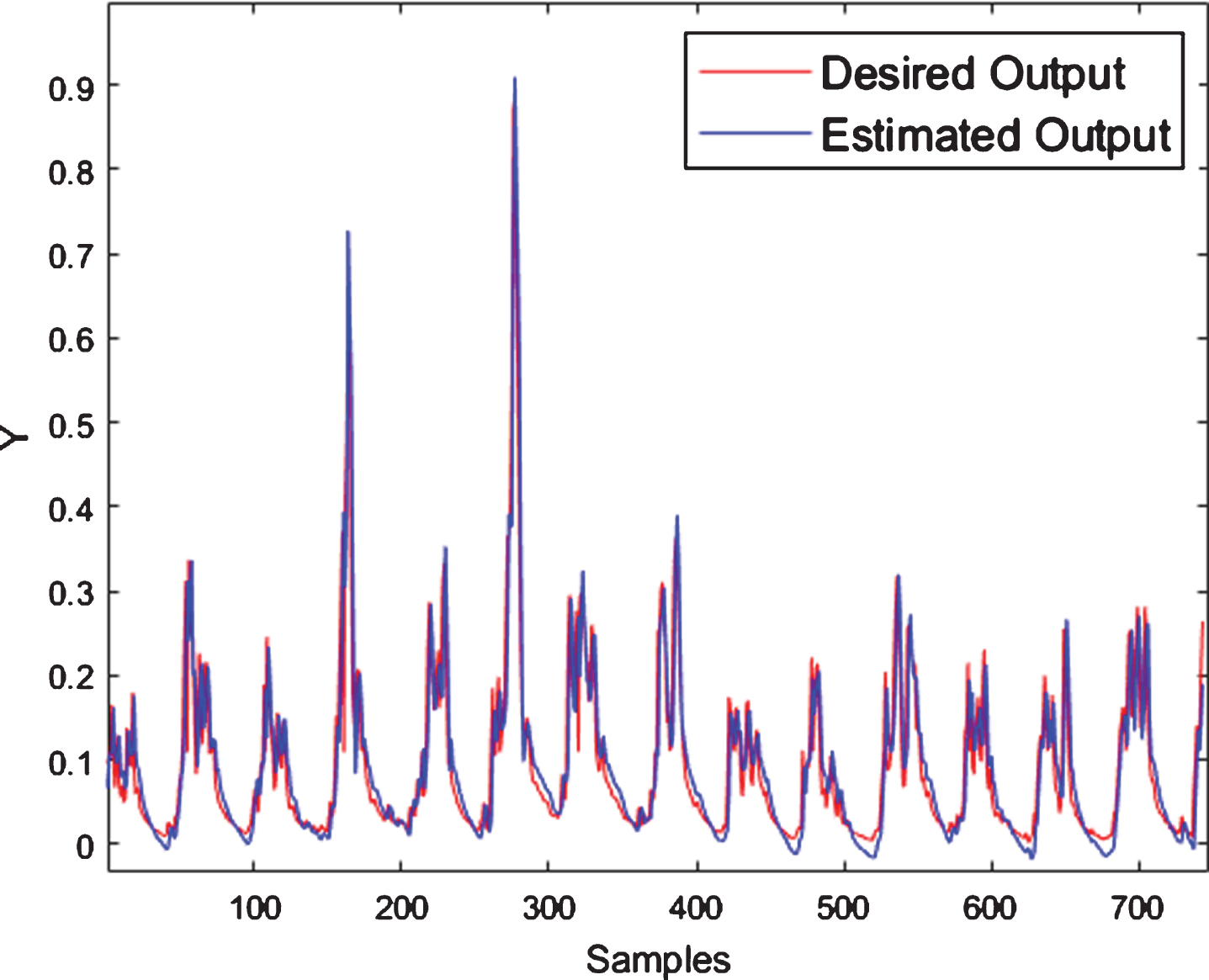
Streamflow forecasting by NFN-MG-GP.

Table 1 shows the RMSE and the standard deviation after all simulation runs. The best performance is achieved by NFN-MG-GP, followed by NFN, ANFIS, and MLP. The results achieved by the NFN-MG-GP and NFN are comparable and outperform those of the other models.

Table 1

Performance of the streamflow forecast models

Model	RMSE (avg)	Stand. Dev
NFN-MG-GP-I	0.0242848	0.0007752
NFN	0.0250892	0.0010261
ANFIS	0.0319734	0.0000000
MLP	0.0962813	0.0186128

Figure 8 shows the boxplot for Streamflow forecasting. It is possible to say NFN-MG-GP’s is statistically superior to MLP and ANFIS since there is no overlap between the corresponding boxes. However, the boxes for NFN-MG-GP and NFN do overlap. So, a pairwise T-test has been executed, obtaining a p-value of 0.01. Since the p-value (0.01) is less than the significance level (0.05), the null hypothesis is rejected, indicating that NFN-MG-GP is statistically better than NFN to this dataset.

Fig. 8

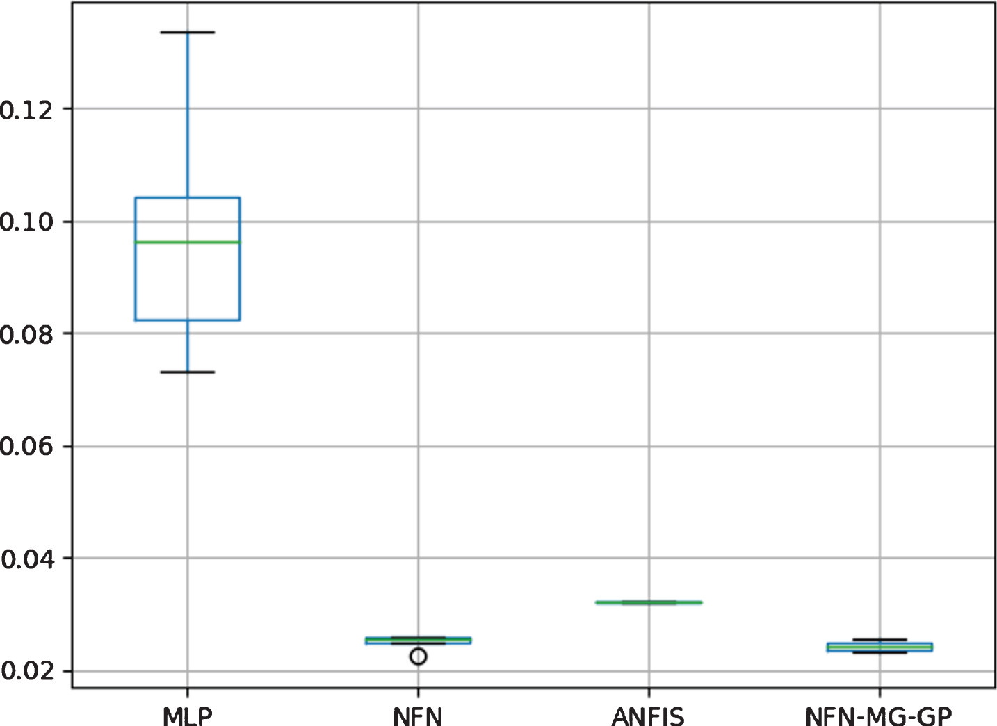
Boxplot to Streamflow forecasting.

5.2 Non-Linear system identification

This experiment aims to analyze the behavior of the proposed algorithms in the non-linear process identification described by: $y_{t} = \frac{y_{t - 1} y_{t - 2} y_{t - 3} (y_{t - 3} - y_{t - 1}) u_{t - 1} + u_{t}}{1 + y_{t - 3}^{2} + y_{t - 2}^{2}},$ (11)

in which y_t = 0 and u_t = 0 for t ≤ 3, u_t is defined by Equation (12) for 3 < t ≤ 500 and by Equation (13) for t > 500: $u_{t} = sin (\frac{2 π t}{250}),$ (12) $u_{t} = sin (\frac{2 π t}{250}) + 0.4 sin (\frac{2 π t}{25}) .$ (13)

The goal is to predict the current output using the delayed input and the outputs. The model for this data set is defined by: ${\hat{y}}_{t} = f (y_{t - 1}, y_{t - 2}, y_{t - 3}, y_{t - 4} y_{t - 5}),$ (14) in which ${\hat{y}}_{t}$ is the output. For the experiment, 10,000 samples are created, 6,000 used to train, 2,000 to validate, and 2,000 to assess their performance by the RMSE. The final membership functions generated by the NFN-MG-GP algorithm are shown in Fig. 9. Figure 10 shows the actual and NFN-MG-GP model outputs for the data.

Fig. 9

Final membership functions for non-linear system identification by NFN-MG-GP.

Fig. 10

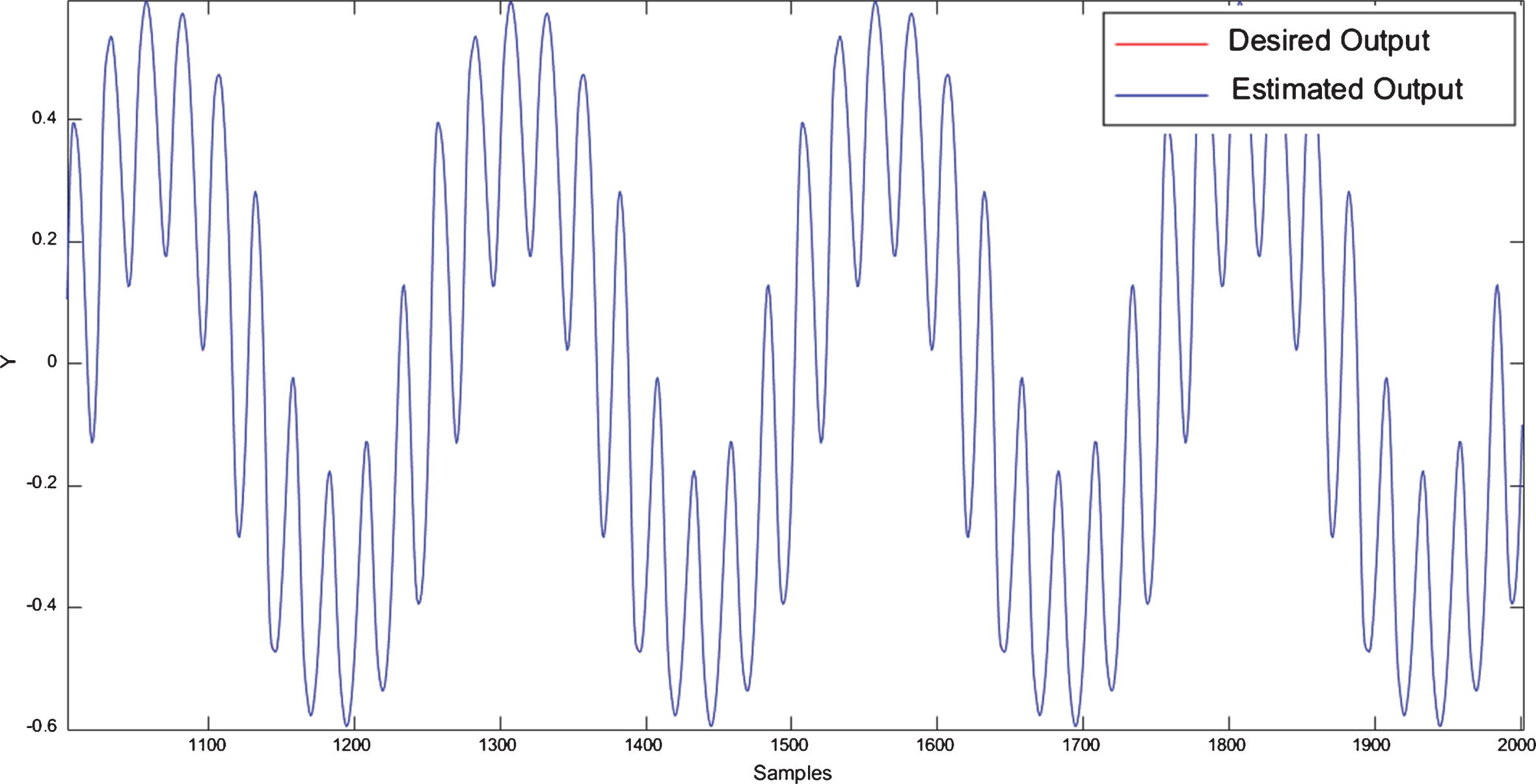
Non-Linear System Identification by NFN-MG-GP.

The RMSE performance of the modeling approaches is summarized in Table 2. They suggest that ANFIS obtains the best performance, followed by NFN-MG-GP and MLP. The results achieved by ANFIS, NFN-MG-GP, and NFN are comparable and are better than the MLP in an order of magnitude.

Table 2

Non-Linear system identification performance

Model	RMSE (avg)	Stand. Dev
ANFIS	0.0000084	0.0000000
NFN-MG-GP	0.0003289	0.0002664
NFN	0.0013669	0.0002830
MLP	0.0766687	0.0230878

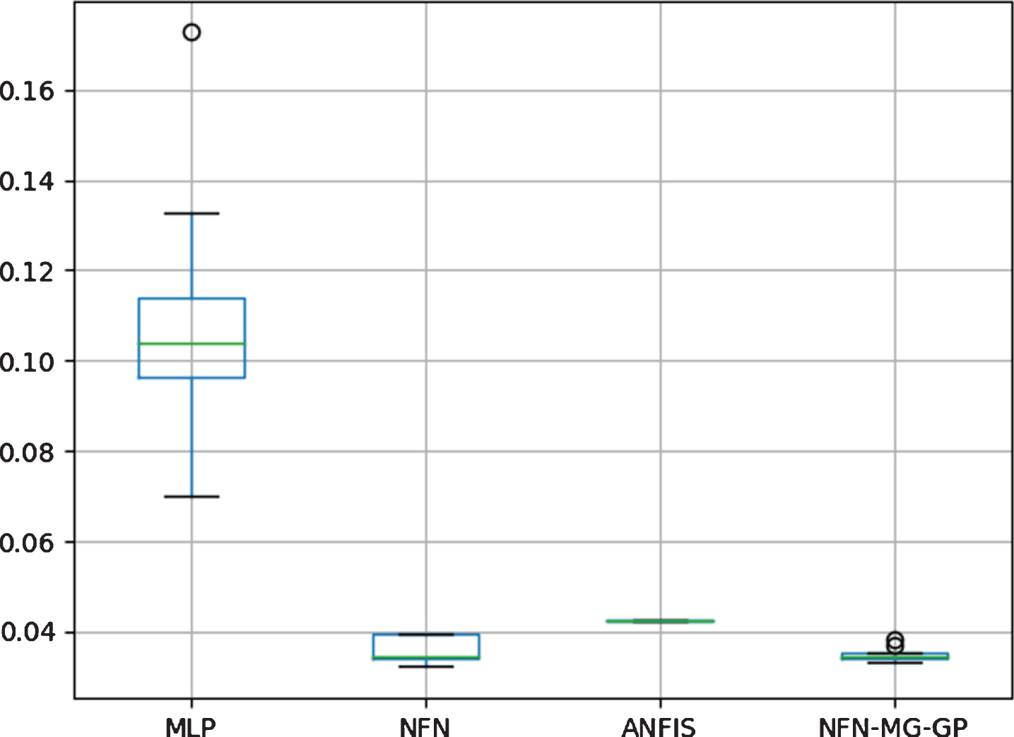
Figure 11 shows the boxplot to Non-Linear System Identification. It is possible to say NFN-MG-GP is statistically superior to NFN and MLP since there is no overlapping between the boxes. Using a different scale, a boxplot presenting the values for NFN-MG-GP and ANFIS are shown in Fig. 12. Since there is no overlapping between the boxes, there is a statistical difference between the two models, being ANFIS superior to NFN-MG-GP.

Fig. 11

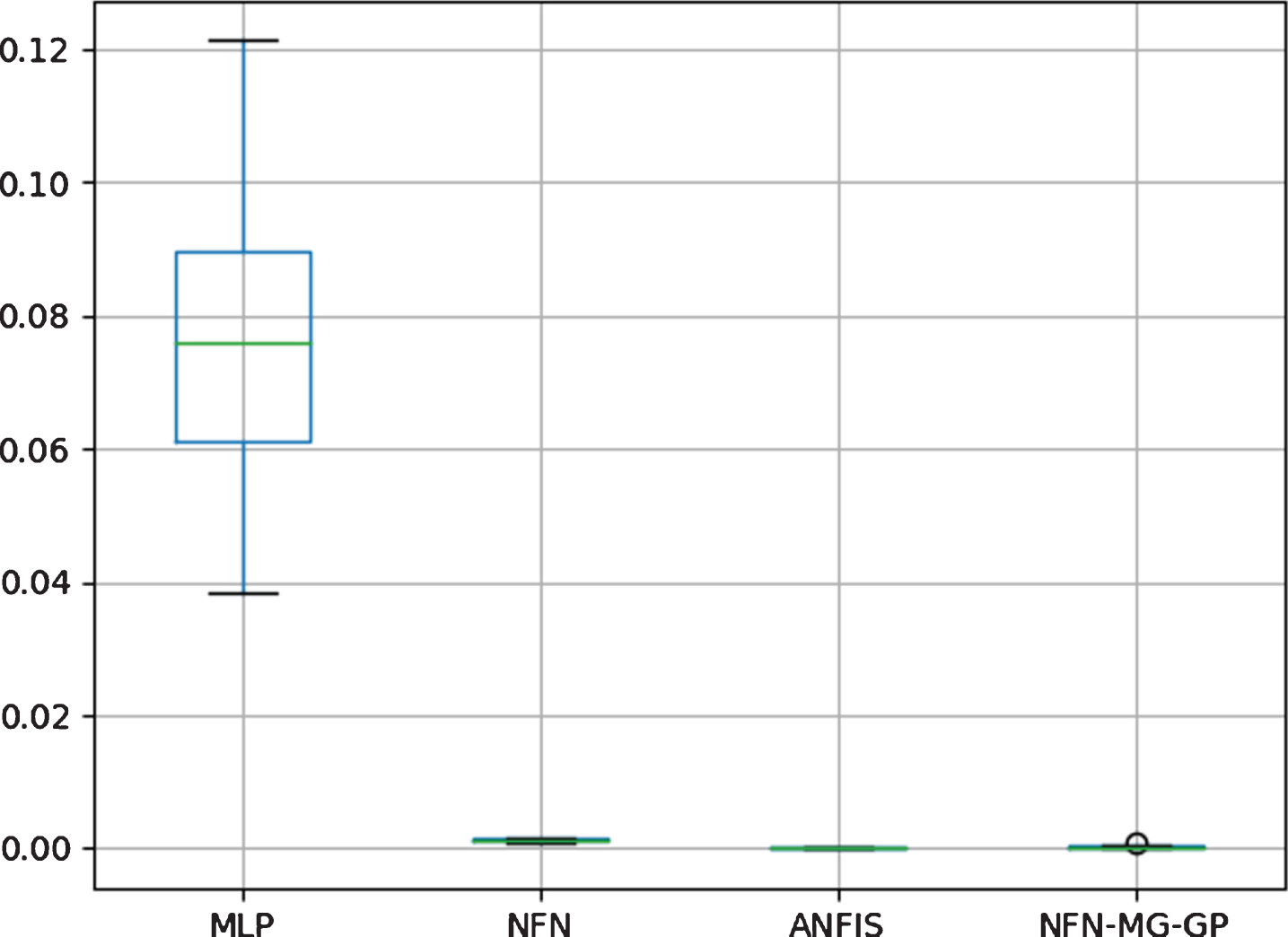
Boxplot to Non-Linear System Identification for all models.

Fig. 12

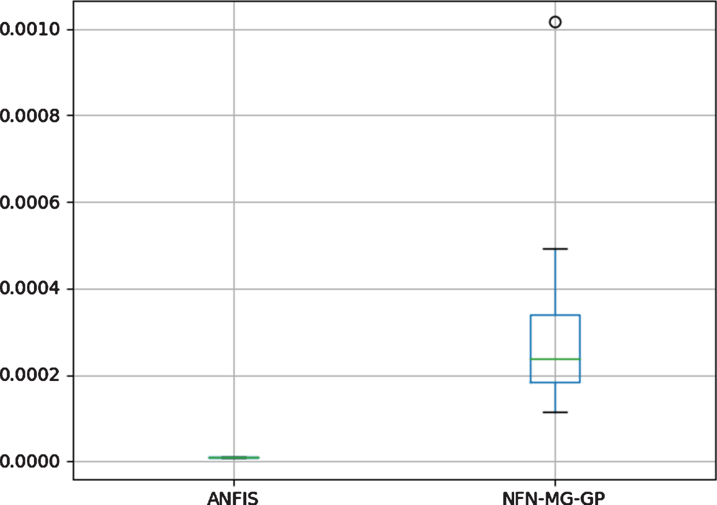
Boxplot for ANFIS and NFN-MG-GP to Non-Linear System Identification using a different scale.

5.3 Temperature prediction in Lisbon

This section evaluates the models to predict the temperature in Lisbon, Portugal, a region with a very varied climate throughout the year, ranging from a very cold winter with snow to a hot summer. The goal is to predict the average monthly temperature one step ahead. Previous work suggests using the first five lagged values of the series as an input [30, 48]. In this way, the model can be described by: $y_{t} = f (y_{t - 1}, y_{t - 2}, y_{t - 3}, y_{t - 4}, y_{t - 5}) .$ (15)

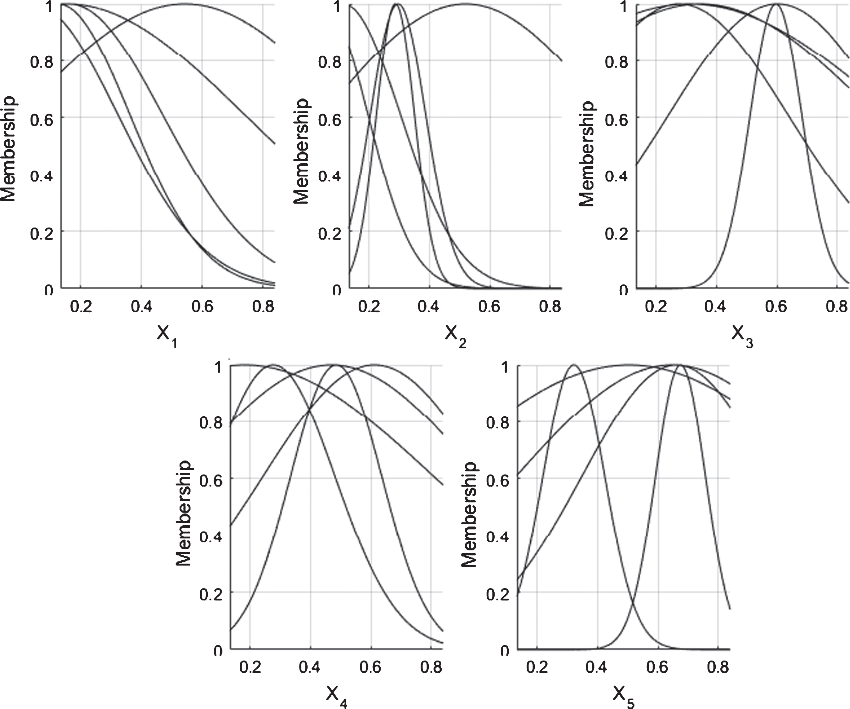
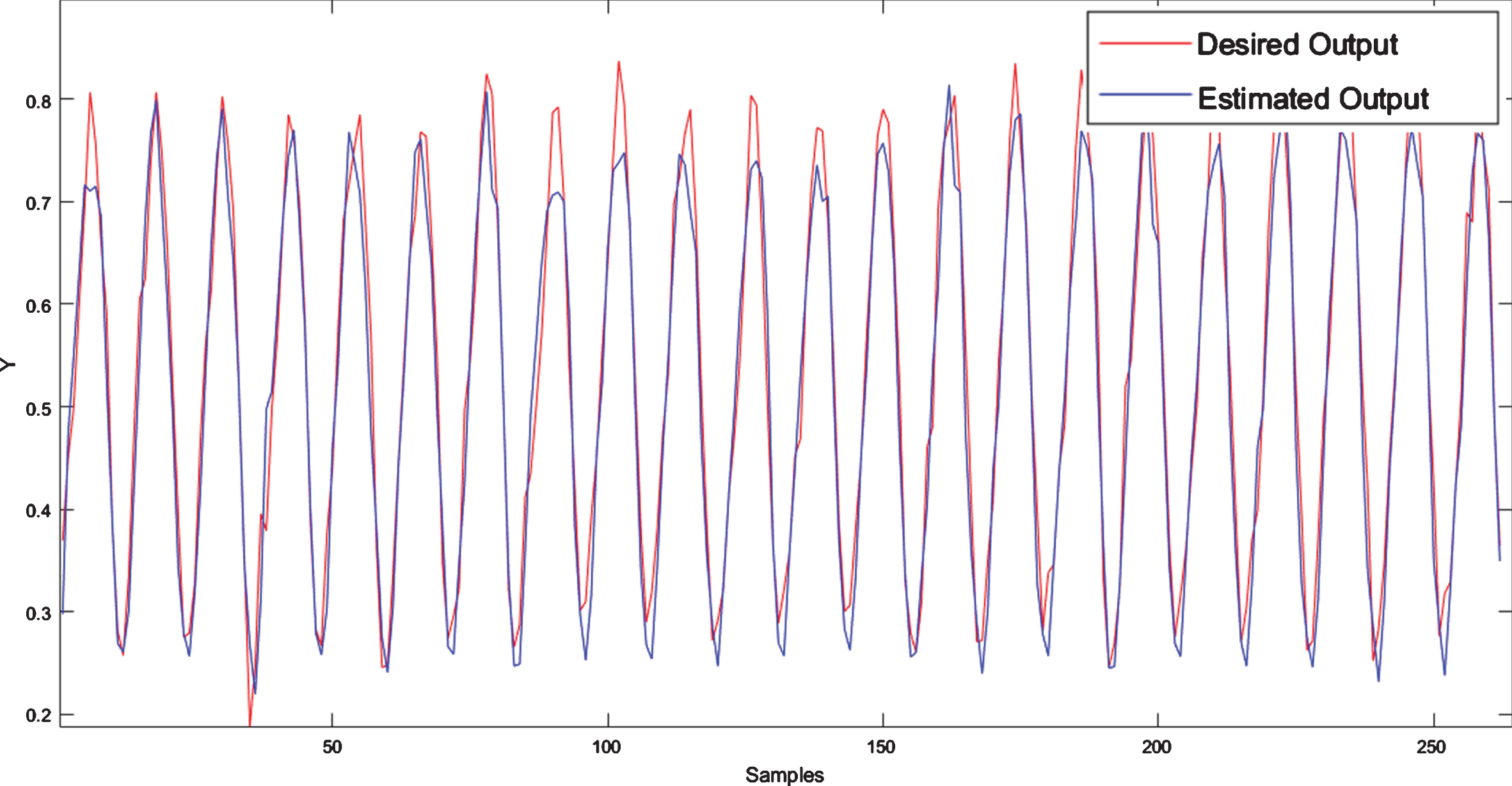
Data refers to the average monthly temperature from January 1910 to December 2009. The data set consists of 1,194 samples, 716 used to train the models, 239 for validation, and 239 for evaluating their performance. Figure 13 shows the membership functions generated by the NFN-MG-GP algorithm, and Fig. 14 depicts the actual value and the forecasted output by NFN-MG-GP.

Fig. 13

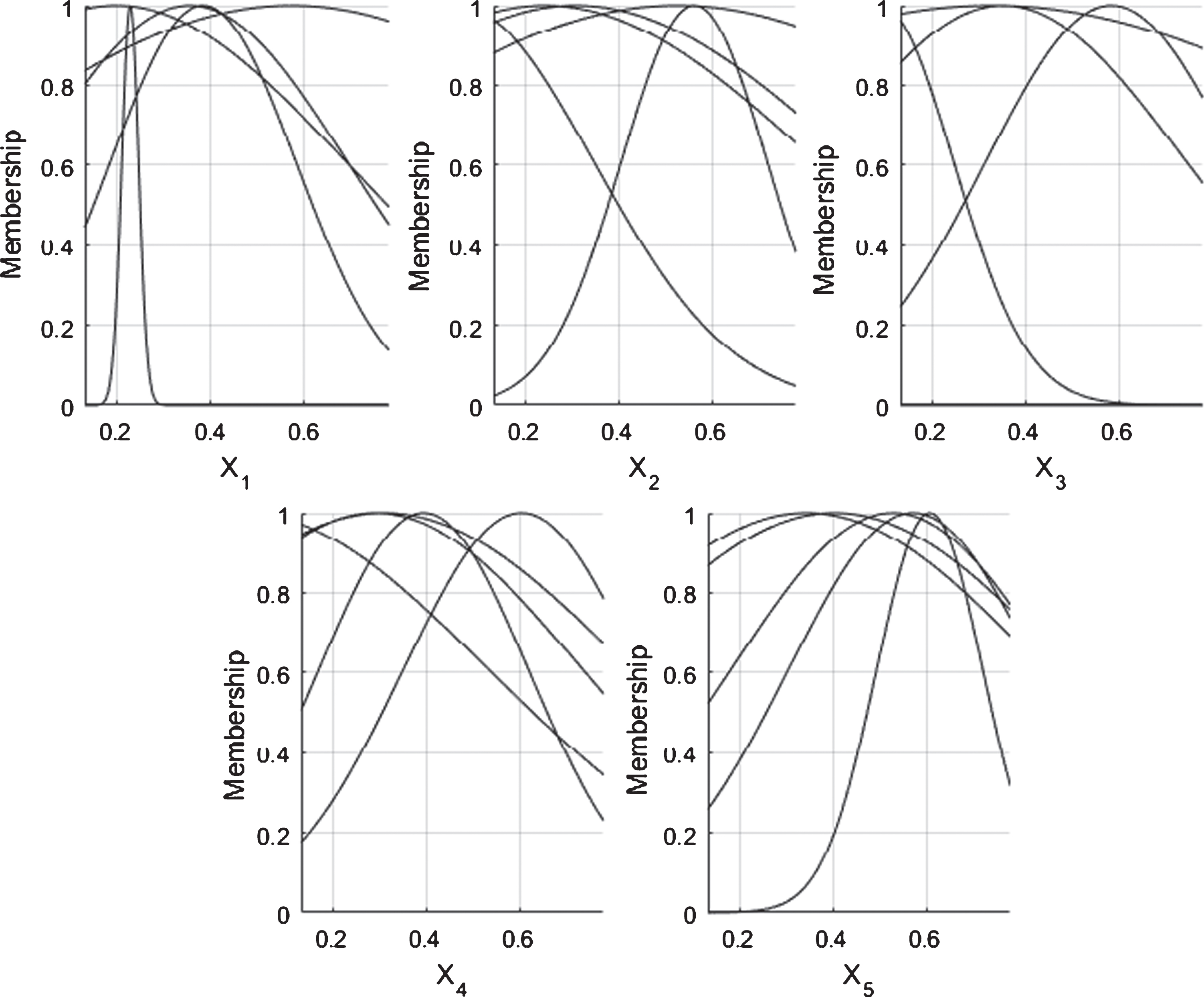
Final membership functions to temperature prediction in Lisbon by NFN-MG-GP.

Fig. 14

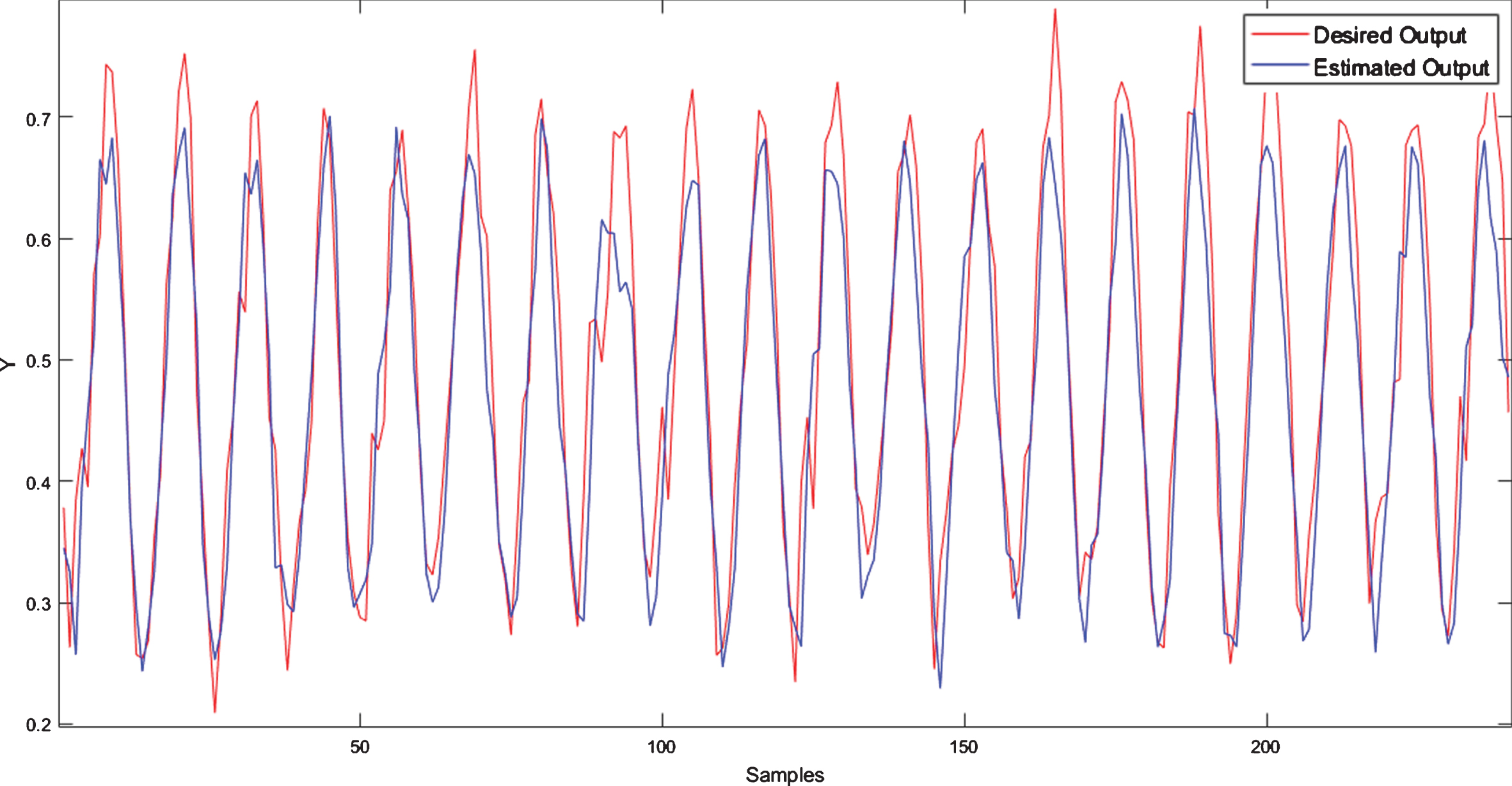
Temperature prediction in Lisbon by NFN-MG-GP.

Table 3 shows the mean and the Standart Deviation of RMSE in temperature prediction in Lisbon. The best performance is obtained by NFN-MG-GP, followed by NFN, ANFIS, and MLP.

Table 3

Temperature prediction in lisbon performance

Model	RMSE (avg)	Stand. Dev
NFN-MG-GP	0.0350318	0.0016136
NFN	0.0361059	0.0029955
ANFIS	0.0426674	0.0000000
MLP	0.1088691	0.0280405

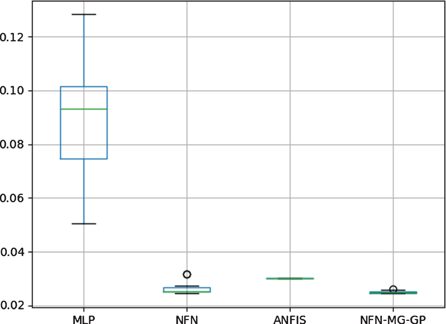
Figure 15 shows the boxplot of RMSE values for a temperature prediction in Lisbon. We can see NFN-MG-GP is better than MLP and ANFIS since any overlapping can be observed between the boxes. The one-tailed T-test between the NFN-MG-GP and NFN has been carried out. With a p-value of 0.17, the null hypothesis cannot be rejected. It indicates that there is no evidence to say NFN-MG-GP is better than NFN.

Fig. 15

Boxplot to Temperature Prediction in Lisbon

5.4 Temperature prediction in death valley

In this experiment, the models are analyzed in temperature prediction in Death Valley, a region with an extremely dry climate and high temperatures. Such as the previous section, the goal is to predict the average monthly temperature one step ahead, according to Equation (15).

The average monthly temperature information for Death Valley spans from January 1901 to December 2009. The data set contains 1,302 samples, of which 781 are used to train the models, 260 to validate, and 261 to evaluate your performance. The final membership functions obtained by the NFN-MG-GP algorithm are illustrated in Fig. 16. Figure 17 presents the desired values and those estimated by the NFN-MG-GP for the evaluation data.

Fig. 16

Final membership functions to temperature prediction in Death Valley by NFN-MG-GP.

Fig. 17

Temperature prediction in Death Valley by NFN-MG-GP.

Table 4 shows the RMSE results obtained by the models for temperature prediction in the Death Valley. The NFN-MG-GP has achieved the best results, followed by NFN, ANFIS, and MLP.

Table 4

Temperature Prediction in Death Valley Performance

Model	RMSE (avg)	Stand. Dev
NFN-MG-GP	0.0250551	0.0005692
NFN	0.0266811	0.0027430
ANFIS	0.0300854	0.0000000
MLP	0.0894537	0.0224695

Figure 18 shows the boxplot for Temperature Prediction in Death Valley. As in the temperature prediction for Lisbon, we can say NFN-MG-GP is statistically superior to MLP and ANFIS. The pairwise comparison between NFN-MG-GP and NFN has been done and, since p - value = 0.0545, the null hypothesis cannot be rejected, indicating that there is no evidence to say NFN-MG-GP and NFN are statistically different.

Fig. 18

Boxplot to Temperature Prediction in Death Valley.

5.5 Discussion

The results presented in this section demonstrate that NFN-MG-GP is able to reach similar or better results than alternative models. In all experiments, NFN-MG-GP showed a better performance than conventional NFN. Thus, the proposed model is efficient for forecasting and non-linear systems identification and competitive with other models. It can be observed that in some cases, some membership functions cover a similar space in the universe of discourse of the input variable. These functions can generate redundancy among rules. It can be seen as a limitation of the proposed algorithm. Despite this limitation, apparently, the performance has not been affected.

6 Conclusion

This work presented a novel approach to building the rule-base of the Neo-Fuzzy-Neuron network. The proposed approach uses Multi-Gene Genetic Programming to create and adjust the rule-base and a Gradient-based method to update the network parameters. Based on this approach, the algorithm NFN-MG-GP was introduced. Multi-Gene Genetic Programming demonstrated an efficient technique to create and adjust the rule-base in NFN networks. This variation of traditional GP facilities the modeling of rule-base by allowing the representation of many functions in the same individual.

Forecast and non-linear system identification application problems were used to evaluate and compare the NFN-MG-GP against current state-of-the-art modeling approaches. Simulation results suggested the NFN-MG-GP has comparable or better performance than the alternative models. The results also showed that the NFN-MG-GP presented less variance when compared with other stochastic models in most cases, which makes the results more consistent.

Future work can address Genetic Programming in network parameters updating, modeling membership functions, and network parameters as individuals from MG-GP. A strategy to eliminate redundant functions should also be studied. The generalization of the model for problems with multiple outputs is also important for future work. Besides, it is possible to consider using triangular membership functions in the NFN network.

Footnotes

Acknowledgement

The authors acknowledges CAPES, Brazilian Ministry of Education, code 001.

References

Abd Elaziz

, Ewees

A.A.

and Alameer

, Improving adaptive neuro-fuzzy inference system based on a modified salp swarm algorithm using genetic algorithm to forecast crude oil price, Natural Resources Research (2019), 1–16.

Abdollahzade

, Miranian

, Hassani

and Iranmanesh

, A new hybrid enhanced local linear neuro-fuzzy model based on the optimized singular spectrum analysis and its application for nonlinear and chaotic time series forecasting, Inf. Sci., 295(C):107–125, Feb. 2015. ISSN 0020-0255. doi: 10.1016/j.ins.2014.09.002.

Abraham

, Neuro fuzzy systems: State-of-the-art modeling techniques. In J. Mira and A. Prieto, editors, Connectionist Models of Neurons, Learning Processes, and Artificial Intelligence, pages 269–276, Berlin, Heidelberg, 2001. Springer Berlin Heidelberg. ISBN 978-3-540-45720-6.

Aryafar

, Khosravi

, Zarepourfard

and Rooki

, Evolvinggenetic programming and other ai-based models for estimatinggroundwater quality parameters of the Khezri plain, Eastern Iran, Environmental Earth Sciences 78(3) (2019), 69.

Ashish

, Dasari

, Chattopadhyay

and HuiGenetic-neuro-fuzzy

N.B.

, system for grading depression, AppliedComputing and Informatics 14(1) (2018), 98–105.

Azad

R.M.A.

and Ryan

, A simple approach to lifetime learning ingenetic programming-based symbolic regression, EvolutionaryComputation 22(2) (2014), 287–317.

Badnjevic

, Cifrek

, Koruga

and Osmankovic

, Neuro-fuzzy classification of asthma and chronic obstructive pulmonary disease, BMC Medical Informatics and Decision Making 15(3):S1, Sep 2015. ISSN1472-6947. doi: 10.1186/1472-6947-15-S3-S1.

Bodyanskiy

and Antonenko.

, Deep neo-fuzzy neural network and its accelerated learning. In 2020 IEEE Third International Conference on Data Stream Mining Processing (DSMP), pages 67–71, 2020. doi: 10.1109/DSMP47368.2020.9204068

Bodyanskiy

, Kulishova

and Malysheva

, The multidimensional extended neo-fuzzy systemand its fast learning for emotions online recognition. In 2018 IEEE Second International Conference on Data Stream Mining & Processing (DSMP), pages 473–477. IEEE, 2018.

10.

Bodyanskiy

, Peleshko

, Rashkevych

and Vynokurova

, The autoencoder based on generalized neofuzzy neuron and its fast learning for deep neural networks. In 2018 IEEE Second International Conference on Data Stream Mining Processing (DSMP), pages 113–118, Aug 2018. doi: 10.1109/DSMP.2018.8478624.

11.

Bodyanskiy

, Boiko

, Zaychenko

, Hamidov

and ZelikmanThe

, The hybrid gmdh-neo-fuzzy neural network in forecasting problems in financial sphere. In 2020 IEEE 2nd International Conference on System Analysis Intelligent Computing (SAIC), pages 1-–6, 2020. doi: 10.1109/SAIC51296.2020.9239152.

12.

Bodyanskiy

Y.V.

and Tyshchenko

O.K.

, A hybrid cascade neuro–fuzzynetwork with pools of extended neo–fuzzy neurons and its deeplearning, International Journal of Applied Mathematics andComputer Science 29(3) (2019), 477–488, 01 Sep. 2019. doi: 10.2478/amcs-2019-0035.

13.

Bodyanskiy

Y.V.

, Tyshchenko

O.K.

and Kopaliani

D.S.

, An extendedneo-fuzzy neuron and its adaptive learning algorithm, International Journal of Intelligent Systems and Applications 7(2) (2015), 21–26. doi: 10.5815/ijisa.2015.02.03.

14.

Caliskan

, Çil

Z.A.

, Badem

and Karaboga

, Regression-based neuro-fuzzy network trained by abc algorithm forhigh-density impulse noise elimination, IEEE Transactions onFuzzy Systems 28(6) (2020), 1084–1095. doi: 10.1109/TFUZZ.2020.2973123.

15.

Cervantes

, Yu

, Salazar

and Chairez

, Takagi–sugenodynamic neuro-fuzzy controller of uncertain nonlinear systems, IEEE Transactions on Fuzzy Systems 25(6):1601–1615, Dec 2017. ISSN 1063-6706. doi: 10.1109/TFUZZ.2016.2612697.

16.

Eray

, Mert

and Kisi

, Comparison of multi-gene geneticprogramming and dynamic evolving neural-fuzzy inference system inmodeling pan evaporation, Hydrology Research 49(4):1221–1233, 11 2017. ISSN 0029-1277. doi: 10.2166/nh.2017.076.

17.

Fernandez

, López

, del Jesus

M.J.

and Herrera

, Revisiting evolutionary fuzzy systems: Taxonomy, applications, newtrends and challenges, Knowledge-Based Systems 80(2015), 109–121. ISSN 0950-7051. doi: 10.1016/j.knosys.2015.01.013.

18.

Ferreira

, Gene expression programming: a new adaptive algorithmfor solving problems, Complex Systems 13(2) (2001), 87–129.

19.

Hernandez

, Castejon

, García-Prada

J.C.

, Padrónand

and Marichal

G.N.

, Wavelet packets transform processing and geneticneuro-fuzzy classification to detect faulty bearing, Advancesin Mechanical Engineering 11(8) (2019).

20.

Herrera

, Genetic fuzzy systems: taxonomy, current research trendsand prospects, Evolutionary Intelligence 1(1) (2008), 27–46. doi: 10.1007/s12065-007-0001-5.

21.

Holland

J.H.

and Reitman

J.S.

, Cognitive systems based on adaptivealgorithms, SIGART Bull. 1(63) (1977), 49–49. ISSN 0163-5719. doi: 10.1145/1045343.1045373.

22.

, Bodyanskiy

Y.V.

and Tyshchenko

O.K.

, A deep cascade neural network based on extended neo-fuzzy neurons and its adaptive learning algorithm. In 2017 IEEE First Ukraine Conference on Electrical and Computer Engineering (UKRCON), pp. 801–805, May 2017.

23.

Karczmarz

, Angenaherte auflosung von systemen linearer glei-chungen, Bull. Int. Acad. Pol. Sic. Let., Cl. Sci. Math. Nat. (1937), 355–357.

24.

Kaur

, Bhardwaj

and Been

U.A.H.

, Genetic neuro fuzzy system forhypertension diagnosis, International Journal of ComputerScience and Information Technologies 5(4) (2014), 4986–4989. ISSN 0975-9646.

25.

Klir

G.J.

and Yuan

, Fuzzy sets and fuzzy logic: theory andapplications, Possibility Theory versus Probab. Theory 32(2) (1996), 207–208.

26.

Koshiyama

A.S.

, Vellasco

M.M.

and Tanscheit

, Gpfis-class: Agenetic fuzzy system based on genetic programming for classificationproblems, Appl. Soft Comput. 37(C) (2015), 561–571. ISSN 1568-4946. doi: 10.1016/j.asoc.2015.08.055.

27.

Kosko

, Fuzzy systems as universal approximators, IEEE Trans.Comput. 43(11) (1994), 1329–1333. ISSN 0018-9340. doi: 10.1109/12.324566.

28.

Kreinovich

, Quintana

and Reznik

, Gaussian membership functions are most adequate in representing uncertainty in measurements. In Proceedings of NAFIPS (1992), 15-–17.

29.

and Pillai

, Regularized extreme learning adaptiveneuro-fuzzy algorithm for regression and classification, Know.-Based Syst. 127(C) (2017), 100–113. ISSN 0950-7051. doi: 10.1016/j.knosys.2017.04.007.

30.

Leite

, Ballini

, Costa

and Gomide

, Evolving fuzzygranular modeling from nonstationary fuzzy data streams, Evolving Systems 3(2) (2012), 65–79. ISSN 1868-6486. doi: 10.1007/s12530-012-9050-9.

31.

Lemos

, Caminhas

and Gomide

, Fuzzy evolving linearregression trees, Evolving Systems 2(1) (2011), 1–14. ISSN 1868-6486. doi: 10.1007/s12530-011-9028-z.

32.

Mendes

, Souza

, Araújo

and Rastegar

, Neofuzzy neuronlearning using backfitting algorithm, Neural Computing andApplications 31 (2019), 3609–3618. doi: 10.1007/s00521-017-3301-4.

33.

Han

Min

, Xi

Jianhui

, Xu

Shiguo

and Yin

Fu-Liang

, Prediction ofchaotic time series based on the recurrent predictor neural network, IEEE Transactions on Signal Processing 52(12) (2004), 3409–3416. doi: 10.1109/TSP.2004.837418.

34.

Mitra

and Hayashi

, Neuro-fuzzy rule generation: survey in softcomputing framework, IEEE Transactions on Neural Networks 11(3) (2000), 748–768.

35.

Mousavi

, Esfahanipour

and Zarandi

M.H.F.

, Mgpintactsky:Multitree genetic programming-based learning of interpretable andaccurate tsk systems for dynamic portfolio trading, AppliedSoft Computing 34 (2015), 449–462. ISSN 1568-4946. doi: 10.1016/j.asoc.2015.05.021.

36.

Nguyen

H.T.

, Kreinovich

and Sirisaengtaksin

, Fuzzy control asa universal control tool, Fuzzy Sets Syst. 80(1) (1996), 71–86. ISSN 0165-0114. doi: 10.1016/0165-0114(95)00263-4.

37.

Nobile

M.S.

, Cazzaniga

, Besozzi

, Colombo

, Mauri

and Pasi

, Fuzzy self-tuning pso: A settings-free algorithm for globaloptimization, Swarm and Evolutionary Computation 39 (2018), 70–85. ISSN 2210-6502. doi: 10.1016/j.swevo.2017.09.001.

38.

Oliveira

L.O.V.

, Otero

F.E.

, Pappa

G.L.

and Albinati

, Sequential symbolic regression with genetic programming. In Genetic Programming Theory and Practice XII, pages 73–90. Springer, 2015.

39.

Omisore

M.O.

, Samuel

O.W.

and Atajeromavwo

E.J.

, Agenetic-neuro-fuzzy inferential model for diagnosis of tuberculosis, Applied Computing and Informatics 13(1) (2017), 27–37.

40.

Pedrycz

, Neurocomputations in relational systems, IEEETrans. Pattern Anal. Mach. Intell. 13(3) (1991), 289–297. ISSN 0162-8828. doi: 10.1109/34.75517.

41.

Poli

, Langdon

W.B.

and McPhee

N.F.

, A Field Guide to Genetic Programming. Lulu Enterprises, UK Ltd, 2008. ISBN 1409200736, 9781409200734.

42.

Precup

R.-E.

, Preitl

, Petriu

, Bojan-Dragos

C.-A.

, Szedlak-Stinean

A.-I.

, Roman

R.-C.

and Hedrea

E.-L.

, Modelbased fuzzycontrol results for networked control systems, Reports inMechanical Engineering 1(1) (2020), 10–25.

43.

Ragmani

, Elomri

, Abghour

, Moussaid

and Rida

, Animproved hybrid fuzzy-ant colony algorithm applied to load balancingin cloud computing environment, Procedia Computer Science 151 (2019), 519–526. ISSN 1877-0509. doi: 10.1016/j.procs.2019.04.070.

44.

Safa

, Sari

P.A.

, Shariati

, Suhatril

, Trung

N.T.

, Wakiland

and Khorami

, Development of neuro-fuzzy and neuro-bee predictivemodels for prediction of the safety factor of eco-protection slopes, Physica A: Statistical Mechanics and its Applications 550 (2020), 124046. ISSN 0378-4371. doi: 10.1016/j.physa.2019.124046.

45.

Setlak

, Bodvanskiy

, Pliss

, Boiko

and Vynokurova

, Deep evolving stacking convex cascade neofuzzy network and its rapid learning. In 2018 Federated Conference on Computer Science and Information Systems (FedCSIS), pages 29–33, Sep. 2018.

46.

Shi

and Mizumoto

, Some considerations on conventionalneuro-fuzzy learning algorithms by gradient descent method, Fuzzy Sets and Systems 112(1) (2000), 51–63. ISSN 0165-0114. doi: 10.1016/S0165-0114(98)00056-6.

47.

Shihabudheen

and Pillai

, Recent advances in neurofuzzy system, Know.-Based Syst. 152(C) (2018), 136–162. ISSN 0950-7051. doi: 10.1016/j.knosys.2018.04.014.

48.

Silva

A.M.

, Caminhas

W.M.

, Lemos

A.P.

and Gomide

, Evolving neural fuzzy network with adaptive feature selection. In 2012 11th International Conference on Machine Learning and Applications, volume 2, pages 440–445, Dec 2012. doi: 10.1109/ICMLA.2012.184.

49.

Silva

A.M.

, Caminhas

, Lemos

and Gomide

, A fast learningalgorithm for evolving neo-fuzzy neuron, Appl. Soft Comput. 14 (2014), 194–209. ISSN 1568-4946. doi: 10.1016/j.asoc.2013.03.022.

50.

Smith

S.F.

, A Learning System Based on Genetic Adaptive Algorithms. PhD thesis, University of Pittsburgh, Pittsburgh, PA, USA, 1980.

51.

Soliman

M.A.

, Hasanien

H.M.

, Azazi

H.Z.

, El-kholy

E.E.

and Mahmoud

S.A.

, Hybrid anfis-ga-based control scheme for performanceenhancement of a grid-connected wind generator, IET RenewablePower Generation 12(7) (2018), 832–843. ISSN 1752-1424.

52.

Takagi

and Sugeno

, Fuzzy identification of systems and its applications to modeling and control, IEEE Transactions on Systems, Man, and Cybernetics, SMC-15(1):116–132, Jan 1985. ISSN 0018-9472. doi: 10.1109/TSMC.1985.6313399.

53.

Terziyska

, Todorov

and Dobreva

, Efficient error based metrics for fuzzy-neural network performance evaluation. In M. Todorov, I. Georgiev, K. Georgiev, and I. Georgiev, editors, Advanced Computing in Industrial Mathematics - 11th Annual Meeting of the Bulgarian Section of SIAM, Revised Selected Papers, Studies in Computational Intelligence, pages 185–201, 1 2018. ISBN 978-331965529-1. doi: 10.1007/978-3-319-65530-7-17.

54.

Wang

, Wang

W.-Y.

, Lee

and Tseng

, Fuzzy b-spline membership function (bmf) and its applications in fuzzy-neural control. Proceedings of the IEEE International Conference on Systems, Man and Cybernetics, 2:2008-–2014, 12 1994. ISSN 0884-3627.

55.

Yamakawa

, Uchino

, Miki

and Kusabagi

, A neo fuzzy neuron and its applications to system identification and predictions to system behavior. In Proceedings of the International Conference on Fuzzy Logic and Neural Networks, pages 477–484. IEEE, 1992. ISBN 0780311043.

56.

Zaychenko

and Hamidov

, The hybrid deep learning gmdh-neo-fuzzy neural network and its applications. In 2019 IEEE 13th International Conference on Application of Information and Communication Technologies (AICT), pages 1–5, 2019. doi: 10.1109/AICT47866.2019.8981725.

57.

Zeng

, Zhang

N.-Y.

and Xu

W.-L.

, A comparative study on sufficientconditions for takagi-sugeno fuzzy systems as universalapproximators, IEEE Transactions on fuzzy systems 8(6) (2000), 773–780.