
Abstract
Multi-granulation decision-theoretic rough sets uses the granular structures induced by multiple binary relations to approximate the target concept, which can get a more accurate description of the approximate space. However, Multi-granulation decision-theoretic rough sets is very time-consuming to calculate the approximate value of the target set. Local rough sets not only inherits the advantages of classical rough set in dealing with imprecise, fuzzy and uncertain data, but also breaks through the limitation that classical rough set needs a lot of labeled data. In this paper, in order to make full use of the advantage of computational efficiency of local rough sets and the ability of more accurate approximation space description of multi-granulation decision-theoretic rough sets, we propose to combine the local rough sets and the multigranulation decision-theoretic rough sets in the covering approximation space to obtain the local multigranulation covering decision-theoretic rough sets model. This provides an effective tool for discovering knowledge and making decisions in relation to large data sets. We first propose four types of local multigranulation covering decision-theoretic rough sets models in covering approximation space, where a target concept is approximated by employing the maximal or minimal descriptors of objects. Moreover, some important properties and decision rules are studied. Meanwhile, we explore the reduction among the four types of models. Furthermore, we discuss the relationships of the proposed models and other representative models. Finally, illustrative case of medical diagnosis is given to explain and evaluate the advantage of local multigranulation covering decision-theoretic rough sets model.
Introduction
Rough sets theory (RS) is an effective soft computing tool proposed by Pawlak [1–3], which is used to analyze and process uncertain information. To date, this theory has been applied to many fields such as feature selection [4–6], knowledge discovery [22–26] and so on [7–10]. After decades of development, rough sets theory (RS) has a great impact on the analysis and treatment of uncertainty [11–13].
In recent decades, in order to meet different needs, rough sets theory has been developed rapidly. According to whether there is fault tolerance, rough sets model can be divided into two types: rough sets model with fault tolerance ability and rough sets model without fault tolerance ability. Rough sets model without fault tolerance includes tolerance rough sets [27], rough fuzzy sets [29], and so on [28, 30]. These models have no fault tolerance and are very sensitive to noise data. Moreover, rough sets model with fault tolerance includes probabilistic rough sets [31], decision-theoretic rough sets [32] and so on [33–36]. These models have fault tolerance and are very reliable when dealing with noise data. Rough sets theory is based on classification, but in real life, equivalence relation is difficult to grasp and get. Based on this situation, Zakowski [37] extended equivalence relation to covering relation and proposed covering rough sets (CRS). As an extension of rough sets model, covering rough sets (CRS) has attracted people’s attention and got many interesting results [19–21, 38–40]. In order to reflect the generality, this paper is based on the covering approximation space.
All the above extension models of rough sets need to consider equivalence classes of all objects in the universe U when calculating approximations of a target concept, and these models are called global rough sets by some scholars. Therefore, it is very time-consuming or even infeasible to use the global rough sets model as a data analysis tool in processing some data sets. Moreover, these global rough sets often require a lot of labeled data. However, with the advent of the era of big data, the amount of available data is rapidly increasing and the scale is getting larger and larger, and it is very time-consuming and sometimes impossible to label these data in the big data environment. Therefore, global rough sets has certain defects for large data sets.
In order to break the limitation of global rough sets, some scholars proposed new data analysis methods based on rough sets theory [14–18]. Qian et al. [46] first proposed local rough sets (LRS). Later, Wang et al. [47] and Qian et al. [48] explored local neighborhood rough sets and local multi-granulation decision-theoretic rough sets (LMGDTRS), respectively, Moreover, Guo et al. [53] studied local logical disjunction double-quantitative rough sets model. The time complexity of calculating the upper and lower approximations of concepts in LRS is always linear, while the time complexity of calculating approximations in the global rough sets is non-linear and very time-consuming. Local rough sets (LRS) can effectively analyze the rough data in large data sets by deeply mining the nature of approximate concepts of the rough sets model. LRS model is the extension and innovation of RS, which has certain fault tolerance capabilities.
In the viewpoint of Granular Computing, an equivalence relation on the universe U is a granularity, and a partition on the universe U can be regarded as a granularity structure. Therefore, Pawlak rough sets is a single granularity rough sets, because the model has only one granular structure (or a single equivalence relation). When the domain of a rough set is divided by multiple equivalence relations, the rough sets model is called multigranulation rough sets (MGRS) [41]. When two attribute subsets in an information system are contradictory or inconsistent, MGRS will show its advantages in knowledge discovery. Combining multigranulation idea and Bayesian decision theory, Qian first studied the multigranulation decision-theoretic rough sets (MGDTRS) [54] and it has become a main research field of rough sets theory. For MGDTRS theory, it not only has the ability of more accurate approximation space description, but also can make more comprehensive evaluations in decision-making processes. Based on these advantages, a series of rough sets models are proposed [43, 49–52]. However, similar to the above global rough sets models, the MGDTRS model also is very time-consuming, because when approximating the target concept, it needs to consider all objects. In view of the above advantages and disadvantages of the MGDTRS model, it is necessary to develop a generalized MGDTRS based on theoretical and experimental analysis to improve the global MGDTRS.
According to the discussion above, in order to improve the global MGDTRS, it is very necessary to study generalized MGDTRS by harnessing the advantage of computational efficiency of local rough sets and the ability of more accurate approximation space description of multi-granulation decision-theoretic rough sets. It is very helpful to combine local rough sets with multi-granulation decision-theoretic rough sets based on the advantage and the ability of these two models.
The main contribution of this paper is that we propose four types of local multi-granulation covering decision-theoretic rough sets (LMGDTRS) models as a generalization of MGDTRS. Those models have strong double fault tolerance capabilities which can adapt to increasing complex environments and provide more comprehensive evaluations in the actual decision-making processes. The purpose of this paper is to improve decision-making ability of MGCRS by combining local rough sets with multi-granulation decision-theoretic rough sets (MGDTRS) based on the advantage of computational efficiency of local rough sets and the ability of more accurate approximation space description of MGDTRS model in covering environment. This is the motivation behind the research presented here. In order to define the target concept approximation in the local multigranulation covering environment, we first define two kinds of local covering decision-theoretic rough sets (LCDTRS) by using the intersection and union of the minimal descriptor of x in the local covering approximation space, which are Type-1 LCDTRS and Type-2 LCDTRS. And then, we propose the Type-1 local multi-granulation covering decision-theoretic rough sets (LMGDTRS) model and Type-2 local multi-granulation covering decision-theoretic rough sets (LMGDTRS) model based on minimal descriptor of x by extending single covering of the universe to multiple covering of the universe. Second, we define two types of local covering decision-theoretic rough sets (LCDTRS) based on the maximal descriptor of x, which are Type-3 LCDTRS and Type-4 LCDTRS. Furthermore, we propose the Type-3 local multi-granulation covering decision-theoretic rough sets (LMGDTRS) model and Type-4 local multi-granulation covering decision-theoretic rough sets (LMGDTRS) model by using the intersection and union of the maximal descriptor of x. Finally, we discuss some properties, reduction among the four types of LMGCRS models, and the relationships of different models.
The rest of this paper is structured as follows. Section 2 provides relevant basic concepts of rough sets theory, multigranulation rough sets, decision-theoretic rough sets, covering rough sets and local rough sets. In Section 3, we introduce four types of local multi-granulation covering decision-theoretic rough sets rough sets (LMGDTRS) models and investigate the basic properties of them. In Section 4, reduction among the four types of LMGCRS models are studied. In Section 5, the relationships of different models are explored. In Section 6, an illustrated case is given to evaluate the advantage of the LMGDTRS model in decision-making processes by comparing it with multigranulation covering rough sets (MGCRS). Finally, Section 7 gets the conclusions and elaborates on future studies.
Preliminaries
In this section, we review some basic concepts such as Pawlak rough sets theory, multigranulation rough sets, decision-theoretic rough sets, covering rough sets and local rough sets.
Pawlak rough sets
We usually use a information system to represent data in rough sets theory. Let a quadruple I = (U, AT, V, f) be an information system, where U is a nonempty universe, AT is all attributes set, V={V a |a ∈ AT} is a nonempty domain of values of attribute a ∈ AT, and f : U × AT → V is a map, this mapping satisfies f (x, a) ∈ V a for any a ∈ AT and any x ∈ U. In speciality, when there are decision attributes in an information system, we call it decision information system. The decision information system is indicated by a tuple: DS = (U, AT ∪ DT, V, f), where DT is decision attribute set, and AT∩ DT = ∅.
In the Pawlak rough sets theory, we have the following basic properties.
(L1)
(L2)
(L3)
(L4)
(L5)
(L6)
(L7)
(L8)
(L9)
Decision-theoretic rough sets
Decision-theoretic rough sets (DTRS) get decision-making based on the minimum Bayesian expected risk. In order to consider the decision risk or enhance the practicability of rough sets decision making. Pawlak and Skowron suggested that rough membership function be used to redefine the upper and lower approximation. The rough membership function μ A is defined as follows:
Next, some basic theories of DTRS model based on rough membership function are reviewed.
Let U be the universe, a set of two states can be got and for each state, a set of three actions about the membership of an object x ∈ X can be taken. The set of states is denoted by Ω = {X, X C } which indicates that an element is in X and not in X, respectively. The set of actions with respect to a state is given by A = {a P , a B , a N }, where P, B and N stand for the three actions in deciding x ∈ pos (X) , x ∈ bn (X), and x ∈ neg (X), respectively. The loss function of risk or action cost in different states is as follows:
Based on the rough membership function μ
A
, object x can be assigned to one of three rough regions(x ∈ pos (X) , x ∈ bn (X), and x ∈ neg (X)) through Bayesian decision-making. The expected loss R (a
i
| [x]
A
) can be obtained as follows.
When λ PP ≤ λ NP < λ BP and λ BN ≤ λ NN < λ PN , the following minimum-risk decision rules can be got:
(P) If P (X| [x] A ) ≥ γ and P (X| [x] A ) ≥ α, decide pos (X);
(N) If P (X| [x] A ) ≤ β and P (X| [x] A ) ≤ γ, decide neg (X);
(B) If β ≤ P (X| [x] A ) ≤ α, decide bn (X).
Where the parameters α, β and γ can be obtained by:
If the condition that (λ PN - λ BN ) (λ NP - λ BP ) ≥ (λ BN - λ NN ) (λ BP - λ PP ) can be satisfied by a loss function, then we have α ≥ γ ≥ β.
Furthermore, when α > β, we can have that α > γ > β, therefore, the decision rules of DTRS can be obtained:
(P) If P (X| [x] A ) ≥ α, decide pos (X);
(N) If P (X| [x] A ) ≤ β, decide neg (X);
(B) If β < P (X| [x] A ) < α, decide bn (X).
Based on these decision rules, the lower and upper approximations of DTRS model can be taken as follows:
If
Pawlak rough sets is based on a single indistinguishable relationship or equivalent relationship to partition the universe. However, multigranulation rough sets (MGRS) is different from Pawlak rough sets in that it divides the universe based on multiple indiscernible relations or equivalent relations. Given an information system I = (U, AT, V, f), A1, A2, ..., A
m
⊆ AT are m attribute subsets, for any subset X of universe U, the lower and upper approximations of optimistic multigranulation rough sets model are denoted as follows [41]:
According to the definition of optimistic multigranulation rough sets model, the lower and upper approximations of pessimistic multigranulation rough sets model are defined as follows as follows:
Let U be a universe of nonempty finite set, and C = {X|X ⊆ U} is a family of non-empty subsets of U. If ∪C = U, then C is called a covering of U.
For any covering on the universe, we can always get its simplest covering, and Md C (x) = MdC-{K} (x) = Mdreduct(C) (x). However, from Definition 2.4, we can obtain the MD C (x) may be different from Mdreduct(C) (x).
In the past few decades, rough sets theory has been greatly developed and improved. However, it is very time-consuming when calculate the upper and lower approximation of a given set, because it needs to consider all equivalent classes in the universe. In order to break this limitation, Qian et al. [46] first proposed local rough sets (LRS) model as follows.
We call the approximate operator pair
In this section, we will discuss the combination of local rough sets (LRS) and multi-granulation decision-theoretic rough sets (MGDTRS) in covering approximation space. Firstly, we extend the covering decision-theoretic rough sets (CDTRS) to local covering decision-theoretic rough sets (LCDTRS) by employing the maximal and minimal descriptors. Secondly, based on LCDTRS, we introduce four kinds of local multi-granulation covering decision-theoretic rough sets (LMGCDTRS) models, which are given by using the minimal descriptors or maximum description of the object x in universe U. Finally, we study some basic properties of four kinds of LMGCDTRS models.
According to the definition of DTRS model, we can see that the conditional function P (·) needs to be given first. In fact, the conditional function P (·) has a lot of forms. Without loss of generality, we select the inclusion degree
Local multi-granulation covering decision-theoretic rough sets based on minimal descriptor
We call the approximation pair
From the above definition of Type-1 LCDTRS model, it can be seen that the calculation of the upper and lower approximation is only based on the information granules determined by the object in the target concept, rather than the information granules from all objects in a given universe, which can greatly reduce the time consumption of calculating the approximation.
According to the above definition, we get the following explanations:
Based on Definition 3.2, we can get that if there is at least one covering C
i
∈
From the above description, we can get the corresponding decision rules of Type-1 LMGCDTRS. The results as follows:
(P) If ∃C
i
such that
(N) If
(UB) If
(LB) If ∃C
i
such that
where Pos (X), Neg (X), Ubn (X), Lbn (X) are the positive region, negative region, upper boundary region, and lower boundary region, respectively.
We call the approximation pair
According to the definition of the Type-2 LCDTRS model given above, the calculation of the lower/upper approximation is based on the information granules in the target concept X, which can significantly reduce the time consumed when computing approximations.
If
From the above definition, we can obtain the following interpretations:
According to Definition 3.4, we can know that if there is at least one covering C
i
∈
Based on the above discussions, we obtain the following decision rules.
(P) If ∃C
i
such that
(N) If
(UB) If
(LB) If ∃C
i
such that
where Pos (X), Neg (X), Ubn (X), Lbn (X) are the positive region, negative region, upper boundary region, and lower boundary region, respectively.
Suppose a subset X = {a, d} and given α = 0.6, β = 0.4, we can obtain the following results from Definition 3.2 and Definition 3.4.
Md C 1 (a) = {K1} Md C 2 (a) = {K4, K6}
Md C 1 (b) = {K1, K2} Md C 2 (b) = {K5}
Md C 1 (c) = {K3} Md C 2 (c) = {K4}
Md C 1 (d) = {K3} Md C 2 (d) = {K7}
And then, we can get that
Furthermore, we can obtain the following results
From Example 1, we can see that the lower and upper approximations of Type-1 LMGCDTRS and Type-2 LMGCDTRS are different with each other. Meanwhile, that means Type-1 LMGCDTRS and Type-2 LMGCDTRS are two kinds of different LMGCDTRS models.
The maximum descriptor of x contains all objects related to x in the approximation space. When we discuss the set approximation problem, the maximum descriptor can provide a detailed and comprehensive description for x in a multi-granulation covering approximation space. According to this, we propose another two types of local multi-granulation covering decision-theoretic rough sets models (LMGCDTRS) based on maximal descriptor, which are called Type-3 LMGCDTRS and Type-4 LMGCDTRS, respectively.
We call the approximation pair
Similar to definition 3.1, it can be seen from the definition of the Type-3 LCDTRS model above, that the model can greatly reduce the time consumption of calculating the approximation.
If
From the above definition, we get the following explanations:
According to Definition 3.6, we can know that if there is at least one covering C
i
∈
According to Definition 3.6 and the above discussions, the decision rules of Type-3 LMGCDTRS model as follows:
(P) If ∃C
i
such that
(N) If
(UB) If
(LB) If ∃C
i
such that
where Pos (X), Neg (X), Ubn (X), Lbn (X) are the positive region, negative region, upper boundary region, and lower boundary region, respectively.
We call the approximation pair
Similar to definition 3.3, we can see that the Type-4 LCDTRS based on maximal descriptors can significantly reduce the time consumed when computing approximations.
If
From the definition we obtain the following interpretations:
Based on Definition 3.6, we can see that if there is at least one covering C
i
∈
According to Definition 3.8 and the above representations, the decision rules of Type-4 LMGCDTRS model as follows:
(P) If ∃C
i
such that
(N) If
(UB) If
(LB) If ∃C
i
such that
where Pos (X), Neg (X), Ubn (X), Lbn (X) are the positive region, negative region, upper boundary region, and lower boundary region, respectively.
MD C 1 (a) = {K1} MD C 2 (a) = {K4, K6}
MD C 1 (b) = {K1, K2} MD C 2 (b) = {K6}
MD C 1 (c) = {K2} MD C 2 (c) {K4}
MD C 1 (d) = {K2} MD C 2 (d) = {K6}
Furthermore, we can get that
Based on the above discussion, we can obtain the following results
From Example 2, we can see that upper and lower approximations of Type-3 LMGCDTRS and Type-4 LMGCDTRS are different with each other. That is to say, that means Type-3 LMGCDTRS and Type-4 LMGCDTRS are different models.
Meanwhile, From Example 1 and Example 2, we can get the conclusion that the approximations of the four types of models are different from each other, in other words, the four types of LMGCDTRS models are also different.
It deserves to point out that, when α = 1 and β = 0, the above Definitions 3.2, 3.4, 3.6, 3.8 will degenerate to multi-granulation covering rough sets (MGCRS). In other words, when
(1)
(2)
(3)
(4)
(1) According to Definition3.2, we know that
Similarly, we have also that
According to Theorem 3.1, we can get that when α = 0.5, β = 0.5, for any subset X ∈ U, the lower and upper approximations of X in each of the above types of LMGCDTRS models satisfy the property of duality.
In the Pawlak rough sets theory, for any X ⊆ U, the approximation operators satisfy the properties (L1) - (L9) and (U1) - (U9) in Section 2.1. We show that eight pairs of approximation operators satisfy the properties in Table 1, where 1 represents “satisfy” and 0 represents “dissatisfy”.
Properties of the eight pairs of approximation operators
From Table 1, we can know that the eight pairs of approximation operators satisfy all the properties in certain conditions, except that L4, U4, U9 do not satisfy the properties.
Next, we will prove part of properties of the eight pairs of approximation operators defined in our LMGCDTRS models in certain conditions.
(1)
(2)
(3)
(4)
(1) According to Definition3.2, we can get that
That means
On the other hand, when
That means,
□
(1)If X ⊆ Y, then
(2)If X ⊆ Y, then
(3)
(4)
(5)
(6)
(1) According to Definition3.2, we get that
(2) According to Definition3.2, we know that
In this section, we will investigate the reduction among the four types of LMGCDTRS models.
<Based on Definition 4.1, we can obtain that for any x ∈ U, C1 ⪯ C2 ⇒ Md C 1 (x) ⊆ Md C 2 (x) and MD C 1 (x) ⊆ MD C 2 (x).
From Definition 3.2 and Definition 4.1, we obtain that
Similarly, we get that
From Theorem 4.1, we can obtain that if C1 ⪯ C2 ⪯ ·· · ⪯ C m , then the lower and upper approximations in multi coverings and lower and upper approximations in the finest covering are the same.
(1)
(2)
(2)
From Theorem 4.2 and Remark 1, we can know that the covering and their corresponding reductions can generate the same upper and lower approximations for Type-1 and Type-2 LMGCDTRS, but it is not true for Type-3 and Type-4 LMGCDTRS.
(1) reduct (C1)= reduct (C3) and reduct (C2)= reduct (C4);
(2) reduct (C1)= reduct (C4) and reduct (C2)= reduct (C3).
we can get that
(1) FCC1+C2 (X) and FCC3+C4 (X) have the same upper and lower approximations.
(2) SCC1+C2 (X) and SCC3+C4 (X) have the same upper and lower approximations.
Based on Definition 2.4 and condition (1), we know that C1 and C3 have the same Md (x), and C2 and C4 have the same Md (x). Therefor, FCC1+C2 and FCC3+C4 have the same upper and lower approximations. In the same way, SCC1+C2 and SCC3+C4 have the same upper and lower approximations. □
Hence, we can obtain that
reduct (C1)= reduct (C3) and reduct (C2)= reduct (C4)
Suppose a subset X = {a, c}, Y = {a, b, c} and given α = 0.6, β = 0.4, we can obtain the following results from Definition 3.2 and Definition 3.4.
(1) reduction (C1)= reduction (C3) and reduction (C2)= reduction (C4);
(2) reduction (C1)= reduction (C4) and reduction (C2)= reduction (C3).
we can get that
(1)TCC1+C2 (X) and TCC3+C4 (X) have the same upper and lower approximations.
(2)UCC1+C2 (X) and UCC3+C4 (X) have the same upper and lower approximations.
□
Relationships of different models
Relationships among the four types of LMGCDTRS models
In this section, we will study the relationships among the four types of LMGCDTRS models proposed in Section 3. In addition, we also discuss some properties of four types of LMGCDTRS models.
According to the definitions of the four types of LMGCDTRS models, the following theorem can be obtained.
(1)
(2) when
(3)
(4) when
From Theorem 5.1, we can see that the four pairs of upper and lower approximations proposed can form a lattice under certain conditions based on the inclusion relation. The lattice among the four types of LMGCRS models is shown in Fig. 1.
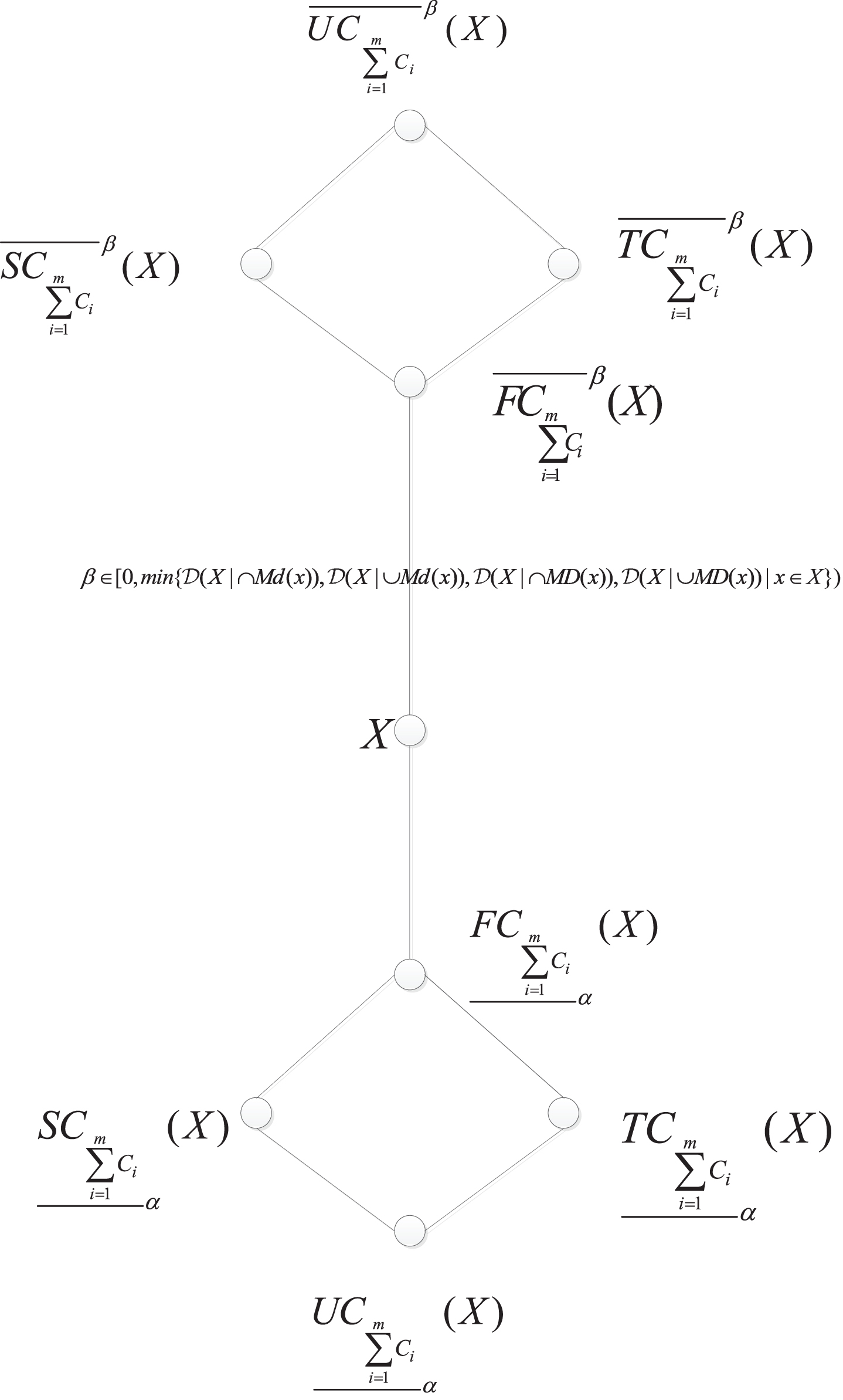
Relationships among four types of LMGCRS models.
From Fig. 1, we can obtain the following some conclusions. When
Furthermore, we can get the following theorem, which contains important conclusions about the relationships among four pairs of upper and lower approximations.
(1)
(2)
(3) when
(4) when
(1)
(2)
□
Theorem 5.3 gives the conditions for the four types of LMGCDTRS models defined in this paper degenerate into MGRS.
According to the above discussions, we research the relationships of the LMGCDTRS model and the four models (RS, DTRS, MGRS and LRS) proposed in the preliminaries. The relationships are shown in Fig. 2.

The relationships of the LMGDTRS, RS, DTRS, MGRS and LRS models.
In Fig. 2, rough sets (RS) lacks fault tolerance due to the strict requirement of set inclusion relationship between equivalence classes and approximate concepts. Based on this shortcoming, decision theoretic rough sets (DTRS) is the quantitative generalization of the qualitative RS. DTRS model quantifies the set inclusion relation based on conditional probability into approximation operator. It is a representative model considering relative quantitative information and approximate concept between equivalent classes, and has certain fault tolerance ability. In practical problems, a domain is not necessarily divided by only one relationship, sometimes the domain is divided by multiple relationships. Multi-granulation rough sets (MGRS) is proposed based on this, which is a natural prolongation of RS when multiple binary relations be considered. When decision risk parameters α = 1, β = 0 and the binary relation is one, both DTRS and MGRS degenerate into RS.
Local rough sets (LRS) can effectively analyze large data sets by mining the essence of approximation concept of rough sets model. LRS model is the extension and innovation of RS, and has certain fault tolerance ability. In 1983, W. Zakowski [37] proposed the generalized rough sets theory based on covering relation by using covering instead of partition on universe. When covering is the partition of universe, the covering rough sets (CRS) degenerates into RS. Based on MGRS and CRS, Liu [45] extend the classical multi-granulation rough sets to multi-granulation covering rough sets (MGCRS). Suppose
Based on the above analysis, the LMGCDTRS model with dual fault tolerance ability can not only describe the approximate space comprehensively, but also meet the requirements of efficient computing.
In this section, we verify the feasibility and validity of the proposed local multi-granulation covering decision-theoretic rough sets (LMGCDTRS) model, and the advantage of the LMGCDTRS model in decision-making processes is verified by comparing it with multigranulation covering rough sets (MGCRS) [45]. In the reference [45], authors proposed four types of multigranulation covering rough sets (MGCRS). In order to prove the effectiveness of the proposed method, we will compare our models with these four types of MGCRS models. We conduct an experiment based on a medical example in literature [42]. These experiments are implemented on a personal computer with Intel Core i3-5005U, 2.00GHz CPU, 8.0GB memory and 64 bit Windows 10 operating system. The software is Matlab R2016a.
Let I = {U, AT, V, f} be a decision information table with multiple granular structures (C1, C2, C3), where U = {x1, x2, ⋯ , x36} represents 36 patients. The condition attributes set {a1, a2} and decision attribute set {d} are fever, headache and cold, respectively. The three granular structures (C1, C2, C3) are covering of U, respectively. The detailed statistics of the datasets are shown in Table 2, where the attribute values 0, 1, 2 denote severity of symptoms, 0 denote not serious, 1 denote serious, 2 denote very serious.
Initial medical data
Initial medical data
Without loss of generality, we use the following subset of U to construct three granular structures (C1, C2, C3).
K1 = {x1, x2, x3, x5, x7, x12, x14, x16, x17, x19,
x22, x23}
K2 = {x3, x4, x10, x11, x15, x16, x18, x19, x20, x25,
x26, x33, x34, x35, x36}
K3 = {x6, x8, x9, x13, x21, x27, x28, x29, x30}
K4 = {x3, x4, x6, x17, x20, x24, x25, x29, x31, x32,
x33, x34, x35}
K5 = {x15, x16, x18, x19, x20, x33}
K6 = {x1, x2, x3, x23}
K7 = {x1, x6, x12, x16, x19, x20, x21, x23, x26, x29,
x31, x34, x36}
K8 = {x2, x4, x5, x9, x10, x11, x12, x14, x17, x18,
x32, x33, x35}
K9 = {x3, x4, x5, x6, x7, x8, x10, x13, x14, x15,
x16, x22, x23, x24, x25, x26, x27, x28, x30}
K10 = {x13, x14, x15, x22, x27}
K11 = {x4, x5, x9, x17, x18}
K12 = {x1, x20, x26}
K13 = {x2, x10, x12, x13, x15, x17, x18, x19, x21,
x23, x24, x27, x30, x32, x35}
K14 = {x1, x3, x4, x5, x6, x7, x8, x9, x11, x14, x16,
x20, x22, x25, x26, x27, x28, x29, x31, x33,
x34, x35, x36}
K15 = {x1, x3, x20, x25, x28, x33, x34, x35}
K16 = {x17, x18, x19, x21, x35}
K17 = {x34, x35}
Then, we obtain that C1 = {K1, K2, K3, K4, K5, K6}, C2 = {K7, K8, K9, K10, K11, K12} and C3 = {K13, K14, K15, K16, K17} are covering on the universe U, respectively. Based on Table 2, we can get 2 decision classes, which can be denoted by U/d = {D1, D2}, where D1 = {x1, x2, x4, x7, x8, x12, x13, x16, x17, x19, x22, x23, x25, x27, x30, x31, x32, x35, x36} and D2 = {x3, x5, x6, x9, x10, x11, x14, x15, x18, x20, x21, x24, x26, x28, x29, x33, x34}. D1 and D2 denote have no cold patients and have a cold patients, respectively. According to the definitions of minimal description and maximal description, we can get minimal and maximal description under each covering C i (i = 1, 2, 3). The results are shown in Table 3 and Table 4.
Minimal description under each covering C i
Maximal description under each covering C i
In the following, D2 is selected as the concept to explain the proposed LMGCDTRS, then we can compute the inclusion degree of four types of LMGCDTRS models under each covering C i with respect to X = D2, which are listed in Table 5 - Table 8. Moreover, Table 9, Table 10 and Table 11 show the upper and lower approximations of the proposed LMGCDTRS models.
The degree of inclusion
The degree of inclusion
The degree of inclusion
The degree of inclusion
The lower and upper approximations approximations of X with respect to α = 0.6 and β = 0.4 .
The lower and upper approximations of X with respect to α = 0.5 and β = 0.3
The lower and upper approximations of X with respect to α = 0.7 and β = 0.5
In order to facilitate the comparisons, we first calculate the lower and upper approximations of X in four types of MGCRS models (see [45]) as follow:
The lower and upper approximations of X = D2 in Type-1 MGCRS are
The lower and upper approximations of X = D2 in Type-2 MGCRS are
The lower and upper approximations of X = D2 in Type-3 MGCRS are
The lower and upper approximations of X = D2 in Type-4 MGCRS are
For the convenience of comparison, these results are shown in Table 12.
The lower and upper approximations of X in four types of MGCRS models
In the Bayesian decision procedure, the decision-making is based on a pair of threshold (α, β). The decision risk parameters α, β is determined by the decision loss function given by the experts in the relevant field and they are generally divided into three situations which α + β = 1, α + β < 1, α + β > 1. Since the rough region of LMGCDTRS model is related to the variable α + β, the theory of LMGCDTRS is expounded from three cases. When the loss function is given, we will be able to discuss decision rules based on different combinations of parameters.
In a loss function, when λ PP = 0, λ PN = 18, λ BP = 9, λ BN = 2, λ NP = 12, λ NN = 0, we can get the decision risk parameters α = 0.6, β = 0.4.
According to the above definitions, we can have the upper and lower approximations of the four types of LMGCDTRS models. The results are shown in Table 9. According to Table 9, we can obtain the rough regions of the four types of model with respect to α = 0.6, β = 0.4. For simplicity and without loss of generality, we choose the rough regions of Type-4 LMGCDTRS as an sample, and the results can be obtained as follows:
Pos (X) = {x11, x26, x28}
Neg (X) = {x1, x2, x5, x7, x12, x13, x14, x17, x19,
x22, x23, x24, x25, x30, x32}
Ubn (X) = {x3, x4, x6, x8, x9, x16, x20, x25, x27,
x29, x31, x33, x34, x35, x36}
Lbn (X) = {x10, x15, x18, x21}
Furthermore, we can get the decision rules by using Type-4 LMGCDTRS model as follows:
(P) The patients x11, x26, x28 have a cold by positive region rule.
(N) The patients x1, x2, x5, x7, x12, x13, x14, x17, x19, x22, x23, x24, x25, x30, x32 have no cold by negative region rule.
(B) The patients x3, x4, x6, x8, x9, x10, x15, x16, x18, x20, x21, x25, x27, x29, x31, x33, x34, x35, x36 cannot be diagnosed, further information is needed.
Based on Table 12, we can obtain the decision rules by using Type-4 MGCRS model as follows:
(P′) It is impossible to judge someone having a cold by positive region rule.
(N′) It is impossible to judge someone having no cold by negative region rule.
(B′) The all patients cannot be diagnosed, further information is needed.
By comparing the two models, we can find that the Type-4 LMGCDTRS model we proposed can accurately determine who has a cold, whereas the Type-4 MGCRS model cannot.
When λ PP = 0, λ PN = 19, λ BP = 12, λ BN = 3, λ NP = 19, λ NN = 0, based on the loss function, we can get α = 0.5, β = 0.3.
According to Table 10, we can directly obtain the rough regions of four types of LMGCDTRS models by the definitions. Without loss of generality, we choose the Type-2 LMGCDTRS as an example, and the rough regions are exhibited by following way.
Pos (X) = {x3, x6, x9, x10, x11, x15, x18, x20, x21,
x24, x26, x28, x29, x33, x34}
Neg (X) = {x1, x2, x7, x12, x22, x23}
Ubn (X) = {x4, x8, x13, x16, x17, x19, x25, x27,
x30, x31, x32, x35, x36}
Lbn (X) = {x5, x14}
And then, based on the decision mechanism of these studies, the following decision rules can be obtained simply.
(P) The patients x3, x6, x9, x10, x11, x15, x18, x20, x21, x24, x26, x28, x29, x33, x34 have a cold by positive region rule.
(N) The patients x1, x2, x7, x12, x22, x23 have no cold by negative region rule.
(B) The patients x4, x5, x8, x13, x14, x16, x17, x19, x25, x27, x30, x31, x32, x35, x36 x34 can not be diagnosed.
From Table 12, we can get the decision rules by using Type-2 MGCRS model as follows:
(P′) It is impossible to judge someone having a cold by positive region rule.
(N′) It is impossible to judge someone having no cold by negative region rule.
(B′) The all patients cannot be diagnosed, further information is needed.
It can be seen from the comparison results of the two models that the Type-2 LMGCDTRS model we proposed is more accurate than the Type-2 MGCRS model in determining which patients are suffering from colds.
when λ PP = 0, λ PN = 21, λ BP = 7, λ BN = 2, λ NP = 9, λ NN = 0, we can get α = 0.7, β = 0.5.
According to Table 11, we can get the rough regions of each rough sets models. Without loss of generality, we take the Type-1 LMGCDTRS model as an illustration, and the rough regions of this model are exhibited as follows:
Pos (X) = {x20, x26, x33}
Neg (X) = {x1, x2, x5, x7, x8, x12, x13, x15, x16,
x17, x18, x19, x21, x22, x23, x24, x25,
x27, x28, x30, x31, x32, x34, x35, x36}
Ubn (X) = {x4, x9, x11}
Lbn (X) = {x3, x6, x10, x14, x29}
Then, the decision rules can be simply achieved based on these studied decision mechanisms as follows:
(P) The patients x20, x26, x33 have a cold by positive region rule.
(N) The patients x1, x2, x5, x7, x8, x12, x13, x15, x16, x17, x18, x19, x21, x22, x23, x24, x25, x27, x28, x30, x31, x32, x34, x35, x36 have no cold by negative region rule.
(B) The patients x3, x4, x6, x9, x10, x11, x14, x29 cannot be diagnosed. We need to make a further diagnosis.
Based on Table 12, we can obtain the decision rules by using Type-1 MGCRS model as follows:
(P′) The patients x3, x6, x14, x20, x26, x29, x33 have a cold by positive region rule.
(N′) The patients x1, x2, x16, x19, x27, x35 have no cold by negative region rule.
(B′) The patients x4, x5, x7, x8, x9, x10, x11, x12, x13, x15, x17, x18, x21, x22, x23, x24, x25, x28, x30, x31, x32, x34, x36 cannot be diagnosed.
From the comparison results of the two models, we can see that the number of patients who cannot be judged and requires further examination in the Type-1 LMGCDTRS model we proposed is less than Type-1 MGCRS model.
According to the comparison of the above three cases, we can clearly see that the four types of LMGCDTRS models we proposed are better than the four types of MGCRS models proposed in reference [45] in decision-making. That is to say, we can make more comprehensive evaluations in the actual decision-making processes based on LMGCDTRS model.
For an information system, rough regions and decision rules depend on parameters to solve different problems. Moreover, based on these case studies, we can get that rough regions and decision rules are different for different thresholds. For the same patient, the decision rules depend on the model and threshold. We choose D2 as the target concept set in case study. When α = 0.6, β = 0.4, we have that patients x1, x2, x5, x7, x12, x13, x14, x17, x19, x22, x23, x24, x25, x30, x32 have no cold in the Type-4 LMGCDTRS model. The patients x5, x14 and x24 are diagnosed as having no cold, but in the original Table 2, they are considered to have a cold. We analyze the symptoms of x5, x14 and x24, and think that there is possibility of misdiagnosis. When the thresholds α = 0.5, β = 0.3, we get that the patients who have a cold are x3, x6, x9, x10, x11, x15, x18, x20, x21, x24, x26, x28, x29, x33, x34. Futuremore, we can conclude that x24 has a cold in Type-2 LMGCDTRS model, but not in the Type-4 LMGCDTRS model. Combined with the x24 symptoms shown in Table 2, we can conclude that x24 is suffering from a cold. For the thresholds are α = 0.7, β = 0.5, patients x1, x2, x5, x7, x8, x12, x13, x15, x16, x17, x18, x19, x21, x22, x23, x24, x25, x27, x28, x30, x31, x32, x34, x35, x36 have no cold in Type-1 LMGCDTRS model. These results are consistent with those in Type-4 LMGCDTRS model. In these models, the set of healthy people is different, but x1, x2, x7, x12, x22, x23 are healthy people diagnosed by Type-1, Type-2 and Type-4 LMGCDTRS. Their symptoms suggest that they must be healthy. We can make some preliminary diagnosis and analysis for patients by using these models. The diagnostic results of different models and thresholds are not completely consistent. Therefore, the appropriate model and threshold should be selected according to the actual needs in practical application.
In order to improve decision-making ability of MGCRS. In this study, we combine local rough sets (LRS) with multi-granulation decision-theoretic rough sets (MGDTRS) based on the advantage of computational efficiency of local rough sets and the ability of more accurate approximation space description of MGDTRS model in the covering approximation space, and propose a new LMGCDTRS model. We establish four types of LMCDTRS models, discuss some interesting properties of these models, and derive decision rules of these models based on Bayesian decision method. Moreover, we also discuss some properties of the reduction of LMGCDTRS model. Meanwhile, the relationships of the LMGCDTRS model and other models are analyzed systematically. Theoretical analyses and experimental results show that: (1) the LMGCDTRS model based on local idea is efficient to compute approximations of concepts; (2) the LMGCDTRS model provides more comprehensive evaluations in the actual decision-making processes. This study builds a bridge between MGDTRS and LRS in covering approximation environment and enriches their theories. At the same time, it is helpful for mining data, discovering knowledge and extracting rules in large-scale data environment. In future works, there are many interesting and important issues to be investigated. For instance, the uncertainty measure of the LMGCDRS model and their applications, the topological properties of LMGCDRS, or LMGCDRS in fuzzy settings.
Footnotes
Acknowledgments
The authors would like to thank the anonymous referees for their valuable comments and helpful suggestions. This work is supported by the National Natural Science Foundation of China (No. 11771111).