Based on decision theory rough sets (DTRSs), three-way decisions (TWDs) provide a risk decision method for solving multi-attribute decision making (MADM) problems. The loss function matrix of DTRS is the basis of this method. In order to better solve the uncertainty and ambiguity of the decision problem, we introduce the q-rung orthopair fuzzy numbers (q-ROFNs) into the loss function. Firstly, we introduce concepts of q-rung orthopair fuzzy β-covering (q-ROF β-covering) and q-rung orthopair fuzzy β-neighborhood (q-ROF β-neighborhood). We combine covering-based q-rung orthopair fuzzy rough set (Cq-ROFRS) with the loss function matrix of DTRS in the q-rung orthopair fuzzy environment. Secondly, we propose a new model of q-ROF β-covering DTRSs (q-ROFCDTRSs) and elaborate its relevant properties. Then, by using membership and non-membership degrees of q-ROFNs, five methods for solving expected losses based on q-ROFNs are given and corresponding TWDs are also derived. On this basis, we present an algorithm based on q-ROFCDTRSs for MADM. Then, the feasibility of these five methods in solving the MADM problems is verified by an example. Finally, the sensitivity of each parameter and the stability and effectiveness of these five methods are compared and analyzed.
Intuitionistic fuzzy set (IFS) [1] is an effective extension of fuzzy sets (FSs). Since IFS can consider both the degree of membership (MD) and the degree of non-membership (NMD) of the elements belonging to the set at the same time, IFS has received extensive attention from decision makers and has achieved fruitful results. However, IFSs have some limitations in the application of MADM. It can only describe the fuzzy phenomenon where the sum of MD and NMD is not greater than 1, but cannot describe the fuzzy phenomenon where the sum of MD and NMD is greater than 1. For this reason, Yager [2] put forward the Pythagorean fuzzy set (PFS) to solve the above mentioned limitations. In PFS, the sum of squares of MD and NMD is real number between zero and one. Decision makers will be constrained by PFS in many practical situations. They do not freely assign MD and NMD according to their own ideas. Therefore, more comprehensive models are needed to deal with these constraints. As an extension of PFS and IFS, Yager [3, 4] proposed q-rung orthopair fuzzy set (q-ROFS). In recent years, many scholars have conducted research on q-ROFSs and obtained some research results [5–11]. Among them, Yager et al. [12] developed OWA and Choquet aggregation operator on q-ROFSs. Under the q-ROFSs model, Du [13] used Minkowski-type distance to measure the distance between MD and NMD to solve multi-attribute group decision making (MAGDM) problem. Liu et al. [14] constructed some new operators on the basis of introducing Bonferroni mean operator into q-ROFSs. Liang [15] used projection-based distance measures and TOPSIS to design a corresponding method to infer TWDs.
Covering-based rough set (CRS) [16] is an extension of the partition of Pawlak RS to the covering of RS. Based on the CRS, many scholars have conducted research from different directions. Researchers have done some researches on covering-based fuzzy rough set (CFRS) [17–22], and some researches on decision-making [23, 24]. Ma [25] introduced the general structure of CFRS. Dąŕeer et al. [26, 27] proposed concepts of fuzzy neighborhoods and fuzzy β-neighborhoods. Hussain [28] proposed an q-ROF TOPSIS method for MADM problems that depend on the Cq-ROFRSs.
In recent years, many results have been achieved in the research of DTRS. The main research directions include attribute reduction [29–33], loss function [34, 35], and several extended models based on DTRSs [36–38]. Yao proposed TWDs, which are new theories derived from DTRSs. The universal set is divide into positive region, boundary region and negative region by TWDs. The TWD is combination of Bayesian decision procedure and DTRSs, which has successfully solved many classification problems. The TWD theory has been applied to many practical fields: cluster analysis [39, 40], risk government decision making [41], medical diagnosis [42], investment decision making [43], MAGDM [44], and so on. Existing researches focused on the loss function matrix and conditional probability to expand the TWDs model. For the determination of conditional probability, Yao and Zhou [45] calculated the conditional probability based on Bayes’ theorem and the naive probabilistic independence. Liu [46] calculated the conditional probability through logistic regression. Liang and Liu [47] presented a new TWD model, which uses hesitant fuzzy sets to measure the loss function. Liang and Liu [48] also used IFS as a new evaluation format of the TWD loss function, and then established a new TWD model. Mandal and Ranadive [49] introduced Pythagorean fuzzy numbers (PFNs) into the loss function matrix. These studies greatly promote the application of TWDs and DTRSs. However, although Mandal and Ranadive [49] have introduced PFNs into the loss function matrix, they did not introduce their model into the q-rung orthopair fuzzy environment, especially Cq-ROFSs. So this paper attempts to study q-ROFCDTRSs model through q-ROF β-neighborhood systems and TWDs. By using the negative and positive characteristic of q-ROFNs, we design five methods to address q-ROFNs and deduce appropriate TWDs. We analyze and compare these five methods, summarize their advantages and disadvantages. Then, we develop an algorithm for deriving TWDs with DTRSs based on q-ROF β-covering. Actually, the q-ROFCDTRS model is a vital tool to handle complexity and uncertainty. In addition, by adjusting the value of 0 ≤ μT (χ) 2 + νT (χ) 2 ≤ 1, it can be seen that q-ROFCDTRS is an extension of covering-based PFDTRS (CPFDTRS). Also by adjusting the value of 0 ≤ μT (χ) + νT (χ) ≤ 1, it is an extension of covering-based IFDTRS (CIFDTRS).
Some main contributions of this work are as follows:
(1) The generalized distance calculation formula based on q-ROFNs is introduced, and the closeness index function of q-ROFNs is proposed based on this distance.
(2) Based on q-ROF β-neighborhood, the concept of q-RO β-neighborhood is proposed, and the conditional probability calculation method of q-ROFCAS is further given.
(3) Aiming at the new uncertainty measure of q-ROFS, the loss function matrix of DTRS is discussed by using q-ROFNs. we construct an q-ROFCDTRS according to the Bayesian decision procedure, and put forward decision rules.
(4) we develop five methods to deduce TWDs with q-ROFCDTRS, including one positive viewpoint, one negative viewpoint and three composite viewpoints.
(5) Based on these five proposed methods, we present an algorithm based on TWDs with q-ROFCDTRSs.
(6) The effectiveness and stability of these five proposed methods are compared; then the sensitivity of related parameters is analyzed.
The rest of this paper is arranged as follows: Section 2 introduces some basic concepts of q-ROFS. some concepts of q-ROF β-covering, q-ROF β-covering approximation space (q-ROFCAS) and q-ROF β-neighborhood are introduced in Section 3. In addition, we discussed the method of obtaining conditional probability. The loss function matrix of DTRS is discussed aiming at the new uncertainty measurement of q-ROFSs by using q-ROFNs, and an q-ROFCDTRS as per Bayesian decision procedure is constructed in Section 4. In Section 5, We further study decision rules and propose 5 methods to deduce TWDs with q-ROFCDTRS. After, we design an algorithm based on q-ROFCDTRS model to solve MADM problems. In Section 6, an example is given to illustrate the application method of the proposed q-ROFCDTRS model in TWDs, and these five methods proposed are compared and analyzed. Section 7 summarizes the paper and explains the future research directions.
Preliminaries
This section briefly introduces some basic concepts of q-ROFS.
Definition 2.1. [3] Let U be a finite universe set. An q-ROFS T on U can be expressed as the following mathematical symbol:
where functions 0 ≤ μT (χ) ≤ 1 and 0 ≤ νT (χ) ≤ 1 denote MD and NMD of χ ∈ U to the set T, respectively, which satisfy 0 ≤ μT (χ) q + νT (χ) q ≤ 1, (q ≥ 1), for all χ ∈ U. represents the degree of indeterminacy of χ to T.
For convenience, an q-ROFN is denoted as T (χ) = (μT (χ) , νT (χ)) for all χ ∈ U.
Definition 2.2. [3, 14] Let Ta = (μa, νa) and Tb = (μb, νb) be two q-ROFNs, then they have the following properties:
(1) ;
(2) ;
(3) ;
(4) , k > 0;
(5) Ta ∩ Tb = (min (μa, μb) , max (νa, νb));
(6) Ta ∪ Tb = (max (μa, μb) , min (νa, νb)).
Definition 2.3. [50] Let Ta = (μa, νa) and Tb = (μb, νb) be two q-ROFNs. The natural quasi-ordering on q-ROFNs is defined as:
Ta ≥ Tb if and only if μa ≥ μb and νa ≤ νb.
Remark 2.1. As can be seen from Definition 2.3 that the q-ROFN q- = (0, 1) is the smallest q-ROFN and the q-ROFN q+ = (1, 0) is the biggest q-ROFN, respectively. We also call q+ = (1, 0) the positive ideal q-ROFN and q- = (0, 1) the negative ideal q-ROFN.
Definition 2.4. [14] Let Ta = (μa, νa) be an q-ROFN, The score function S (Ta) and the corresponding accuracy function H (Ta) are defined as follows:
It is easy to get -1 ≤ S (Ta) ≤ 1 and 0 ≤ H (Ta) ≤ 1.
Based on the Definition 2.4, Liu and Liu [14] proposed comparison rules for q-ROFNs as follows:
(1) If S (Ta) > S (Tb), then Ta > Tb;
(2) If S (Ta) < S (Tb), then Ta < Tb;
(3) If S (Ta) = S (Tb), then:
(i) If H (Ta) > H (Tb), then Ta > Tb;
(ii)If H (Ta) < H (Tb), then Ta < Tb;
(iii)If H (Ta) = H (Tb), then Ta = Tb.
Definition 2.5. [51] Let Ta = (μa, νa) and Tb = (μb, νb) be two q-ROFNs, the generalized distance between Ta and Tb is defined as follows:
where , . p ∈ [0, 1] andλ > 0.
Based on the Definition 2.5, we can get the distance between the q-ROFN Ta = (μa, νa) and the q-ROFN q+ = (1, 0) as follow:
and the distance between the q-ROFN Ta = (μa, νa) and the negative ideal q-ROFN q- = (0, 1) as follow:
Normally, if the distance d (Ta, q+) is smaller, then the q-ROFN Ta is larger. On the contrary, if the distance d (Ta, q-) is larger, then the q-ROFN Ta is larger. Based on the idea of TOPSIS [52], we present a concept of closeness index for q-ROFNs.
Definition 2.6. Assume Ta = (μa, νa) be an q-ROFN, q+ = (1, 0) be the positive ideal q-ROFN and q- = (0, 1) be the negative ideal q-ROFN, then the closeness index of Ta is defined as follows:
Apparently, if Ta = q-, then ϑ (Ta) = 0; if Ta = q+, then ϑ (Ta) = 1. And it is easy to observe that 0 ≤ ϑ (Ta) ≤ 1.
For two q-ROFNs Ta = (μa, νa) and Tb = (μb, νb), if ϑ (Ta) ≥ ϑ (Tb), then Ta ≥ Tb.
Li [53] defined a new score function δ (Ta) as follows:
Definition 2.7. [53] Let Ta = (μa, νa) be an q-ROFN, then the new score function δ (Ta) is defined as:
where 0 ≤ δ (Ta) ≤ 1.
Basic concept of Cq-ROFRSs
In this section, we introduce concepts of q-ROF β-covering, q-rung orthopair fuzzy β-covering approximation space (q-ROFCAS) and q-ROF β-neighborhood.
Definition 3.1. [28] (1) Assume U is an universe set, , where q-ROF(U) and k ∈ {1, ⋯ , n}. For any q-ROFN β = (μβ, νβ), if
for all χ ∈ U, then is called an q-ROF β-covering of U. The is called an q-ROFCAS.
(2) Let be an q-ROFCAS, be an q-ROF β-covering of U, β = (μβ, νβ). Then
is called an q-ROF β-neighborhood of χ in U, where k = 1, 2, ⋯ , n.
Based on the q-ROF β-neighborhood , The q-RO β-neighborhood is defined as follows.
Definition 3.2. Let is an q-ROF β-covering on U. is an q-ROF β-neighborhood of χ in U. For an q-ROFN β = (μβ, νβ), χ ∈ U, q-RO β-neighborhood of χ is defined as follow:
Definition 3.3. Let be an q-ROFCAS. X ⊆ U, χ ∈ X, The conditional probability of X relative to is defined as follow:
Obviously, for all χ ∈ U.
From Definition 3.2 and 3.3, it is easy to get the following conclusions.
Proposition 3.1. Let be an q-ROFCAS. X, Z ⊆ U, Xi ⊆ U, where i = 1, 2, ⋯ , m. We can get that
(1) ;
(2) X ⊆ Z implies ;
(3) If Xi is a partition of U, then , where i = 1, ⋯ , m.
Proposition 3.2. Let be an q-ROFCAS. These following properties always hold:
(1)
,
;
(2) X ⊆ Z implies
,
.
Example 3.1. Suppose that be an q-ROFCAS and is a set of q-ROFSs, let q = 4, where U = {χ1, χ2, ⋯ , χ6}, β = (0.8, 0.7). Details are shown in Table 1.
q-ROF β-covering in Example 3.1
χ1
(0.87, 0.6)
(0.83, 0.45)
(0.76, 0.8)
(0.55, 0.89)
(0.6, 0.3)
χ2
(0.78, 0.71)
(0.9, 0.39)
(0.77, 0.6)
(0.82, 0.7)
(0.72, 0.84)
χ3
(0.93, 0.59)
(0.7, 0.79)
(0.95, 0.58)
(0.69, 0.35)
(0.65, 0.89)
χ4
(0.89, 0.69)
(0.7, 0.88)
(0.6, 0.8)
(0.9, 0.35)
(0.9, 0.38)
χ5
(0.69, 0.8)
(0.89, 0.42)
(0.7, 0.82)
(0.9, 0.59)
(0.35, 0.79)
χ6
(0.9, 0.6)
(0.59, 0.89)
(0.89, 0.6)
(0.8, 0.69)
(0.55, 0.9)
From Table 1, we can get is an q-ROF β-covering of U. Then , , , , , .
These calculation results of q-ROF β-neighborhood are shown in Table 2.
q-ROF β-neighborhood in Example 3.1
χ1
χ2
χ3
χ4
χ5
χ6
χ1
(0.83, 0.6)
(0.78, 0.71)
(0.7, 0.79)
(0.7, 0.88)
(0.69, 0.8)
(0.59, 0.89)
χ2
(0.55, 0.89)
(0.82, 0.7)
(0.69, 0.79)
(0.7, 0.88)
(0.89, 0.59)
(0.59, 0.89)
χ3
(0.76, 0.8)
(0.77, 0.71)
(0.93, 0.59)
(0.6, 0.8)
(0.69, 0.82)
(0.89, 0.6)
χ4
(0.55, 0.89)
(0.72, 0.84)
(0.65, 0.89)
(0.89, 0.69)
(0.35, 0.8)
(0.55, 0.9)
χ5
(0.55, 0.89)
(0.82, 0.7)
(0.69, 0.79)
(0.7, 0.88)
(0.89, 0.59)
(0.59, 0.89)
χ6
(0.55, 0.89)
(0.77, 0.71)
(0.69, 0.59)
(0.6, 0.8)
(0.69, 0.82)
(0.8, 0.69)
Then, according to Definition 3.2, we can obtain q-RO β-neighborhoods as follows:
, ,
, ,
, .
Let the decision set X = {χ1, χ3, χ5, χ6}, then we can obtain these conditional probabilities as:
,
,
,
,
,
.
q-ROF β-covering decision-theoretic rough set model
For the new uncertainty measurement of q-ROFSs, we will discuss the loss function matrix of DTRS with q-ROFNs in this section, and construct an q-ROFCDTRS as per Bayesian decision procedure [34, 48].
Based on the Bayesian decision procedure and results of Liang and Liu in the Ref [48], we can conclude that the q-ROFCDTRS consists of two states and three actions. These two states are expressed as Γ = Γ (D, ¬ D). And, these three actions are expressed as , in which bP, bB and bN represent three actions to classify the object χ, that is, determine χ ∈ POS (D), determine χ ∈ BND (D) and determine χ ∈ NEG (D), respectively. They have different semantics according to different decision-making problems. Under the q-rung orthopair fuzzy environment, Liang [15] constructed a loss function matrix involving behavioral risks or costs in the two states. The loss function matrix is shown in Table 3.
The loss function matrix with q-ROFNs
D
¬D
bP
T (λPP) = (μT (λPP) , νT (λPP))
T (λPN) = (μT (λPN) , νT (λPN))
bB
T (λBP) = (μT (λBP) , νT (λBP))
T (λBN) = (μT (λBN) , νT (λBN))
bN
T (λNP) = (μT (λNP) , νT (λNP))
T (λNN) = (μT (λNN) , νT (λNN))
As shown in Table 3, Those loss functions T (λ♦♦) (♦ = P, B, N) are q-ROFNs. In order to write concisely, we make (♦ = P, B, N), and the same description is used in the following parts of this paper, so it will not be explained again. When the object y is in the state D, its loss degrees based on q-ROFNs are T (λPP), T (λBP) and T (λNP) incurred for taking actions of bP, bB and bN. Similarly, when the object χ is not in the state D, its loss degrees based on q-ROFNs are T (λPN), T (λBN) and T (λNN) incurred for taking the same actions. By using the semantics of TWDs and the properties of q-ROFN [15], those loss functions represented in Table 3 have the following relationship:
Proposition 4.1.[15] Based on the relationship of loss functions (10) to (13), we can deduce the following results:
From Proposition 4.1, as can be seen from Equation (14), if the object χ belongs to D, the loss of classifying it into POS (D) is less than or equal to that of classifying it into BND (D). And the loss of classifying it into BND (D) is less than or equal to that of classifying it into NEG (D) [48]. In the same way, the relationship (15) can be explained.
Suppose that is the conditional probability in which the object χ belonging to D is described by its q-RO β-neighborhood . There exists a relationship . Now, for every χ ∈ U, these corresponding expected losses can be expressed as follows.
Proposition 4.2. Because , so (16)-(18) can be re-expressed as follows:
Proposition 4.3. Expected losses can be calculated as follows.
From Proposition 4.3, these following conclusions can be drawn:
Proposition 4.4. According to (22)-(24), expected losses are denoted as follows.
Based on results reported in Ref. [47] and those loss functions in Table 3, we analyze variations in elements of expected losses.
Proposition 4.5.When is constant, μ♦ is non-monotonic, and it decreases as μT (λ♦P) and μT (λ♦N) increase.
Proof. We consider independent variables of μ♦ to be μT (λ♦P) and μT (λ♦N). Then we calculate partial derivatives of μ♦ to μT (λ♦P) and μ♦ to μT (λ♦N). Therefore, when μT (λ♦N) are constants, this calculation process of the partial derivative of μ♦ to μT (λ♦P) is as follow:
Similarly, when μT (λ♦P) are constants, the calculation process of the partial derivative of μ♦ to μT (λ♦N) is as follow:
Because and are established, So the conclusion in Proposition 4.5 holds. □
Proposition 4.6.When is a constant, and ν♦ are non-monotonic, and it decreases as νT (λ♦P) and νT (λ♦N) increase.
Proof. Similar to the proof of Proposition 4.5, We consider independent variables of ν♦ to be νT (λ♦P) and νT (λ♦N). Then we calculate partial derivatives of ν♦ to νT (λ♦P) and ν♦ to νT (λ♦N). Therefore, when νT (λ♦N) are constants, the calculation process of the partial derivative of ν♦ to νT (λ♦P) is as follow:
Similarly, when νT (λ♦P) are constants, the calculation process of the partial derivative of ν♦ to νT (λ♦N) is as follow:
Because there are and , so the conclusion in Proposition 4.6 holds. □
From those conclusions of propositions 4.5 and 4.6, and inspired by these following Refs [34, 55], according to the Bayesian decision-making process, we give minimum cost decision rules in the q-ROF environment as follows:
(P) If and , decide χ ∈ POS (D);
(B) If and , decide χ ∈ BND (D);
(N) If and , decide χ ∈ NEG (D).
Where are q-ROFNs.
On the basis of above results, researches on (P) - (N) are further conducted by using formulas (22)-(24).
Decision-making analysis of q-ROFCDTRS
We will construct an q-ROFCDTRS model, and put forward decision rules in this section. Since expected losses of q-ROFCDTRS cannot be directly compared, it is necessary to further study (P) - (N) according to the operation rules of q-ROFNs. An q-ROFN characterized both by a MD and a NMD, provides two methods for evaluating decision-making problems, one is a positive viewpoint and the other is a negative viewpoint [1, 56]. Next, we will develop five methods to deduce TWDs with q-ROFCDTRS. In this section all
Method 1: A positive viewpoint
In (P) - (N), expected losses are q-ROFNs. In this section, we directly use MDs of q-ROFNs to represent expected losses. Therefore, (P) - (N) are redefined as:
(P1) If and , decide χ ∈ POS (D);
(B1) If and , decide χ ∈ BND (D);
(N1) If and , decide χ ∈ NEG (D);
Under conditions of (10) and (12), we simplify (P1) - (N1). The condition in (P1) is expressed as:
In the same way, for the rule (P1), its second condition is expressed as:
For the rule (B1), the first condition is exactly opposite to the first condition of (P1). It is expressed as:
We get the second condition of rule (B1) as:
For the rule (N1), the first condition is opposite to the second condition of rule (P1) and the second condition is opposite to the second condition of rule (B1). It is expressed as:
Based on the derivation of (P1) - (N1), we express each expression under (P1) - (N1) through three thresholds as follows:
Therefore, (P1) - (N1) can be re-expressed as:
(P1) If and , decide χ ∈ POS (D);
(B1) If and , decide χ ∈ BND (D);
(N1) If and , decide χ ∈ NEG (D);
Based on the positive viewpoint discussed in this section, by comparing thresholds (α1, β1, γ1) and the conditional probability , decision rules of the object χ are finally determined.
Method 2: A negative viewpoint
are expected losses of decision rules (P) - (N). In this section, we use NMDs of q-ROFNs to analyze (P) - (N). In this case, the larger the NMD, the smaller the expected loss. Therefore, (P) - (N) are redefined as:
(P2) If and , decide χ ∈ POS (D);
(B2) If and , decide χ ∈ BND (D);
(N2) If and , decide χ ∈ NEG (D);
Based on conditions (11) and (13), we can simplify (P2) - (N2). For the first condition in (P2) can be simplified to:
Similarly, For (P2), its second condition can be simplified to:
For the rule (B2), its first condition is opposite to the first condition of (P2). It is re-expressed as:
We can get the second condition of (B2) as:
For the rule (N2), its first condition is opposite to the second condition of (P2), and its second condition is opposite to the second condition of rule (B2). It is re-expressed as:
Based on derivations of (P2) - (N2), we express each expression under (P2) - (N2) through three thresholds as follows:
Therefore, (P2) - (N2) are re-expressed as:
(P2) If and , decide χ ∈ POS (D);
(B2) If and , decide χ ∈ BND (D);
(N2) If and , decide χ ∈ NEG (D);
Based on the negative viewpoint discussed in this section, decision rule of the object y are finally determined by comparing thresholds (α2, β2, γ2) and the conditional probability .
Comparing decision rules (P1) - (N1) with (P2) - (N2), the following proposition is obtained.
Proposition 5.1.If πT (λ♦♦) = 0 are true, we get that (P1) - (N1) derived from the positive viewpoint are consistent with (P2) - (N2) derived from the negative viewpoint.
Proof. Based on Definition 2.1 and πT (λ♦♦) = 0, , we deduce the following relationships: νT (λPP) q = 1 - μT (λPP) q, νT (λBP) q = 1 - μT (λBP) q, νT (λNP) q = 1 - μT (λNP) q, νT (λPN) q = 1 - μT (λPN) q, νT (λBN) q = 1 - μT (λBN) q and νT (λNN) q = 1 - μT (λNN) q. With above relationships, thresholds (α2, β2, γ2) are recalculated as:
In this case, thresholds (α2, β2, γ2) correspond to thresholds (α1, β1, γ1) of (P1) - (N1). The statement in Proposition 5.1 holds. □
For Proposition 5.1, the condition μT (λ♦P) q + νT (λ♦P) q = 1 ensures the consistency between (P1) - (N1) and (P2) - (N2). Take the case of T (λPP) = (μT (λPP) , νT (λPP)), the relationship between μT (λPP) and νT (λPP) is shown by the case (1) of Fig. 1.
The relationship between μT (λPP) and νT (λPP).
However, under actual circumstances, condition μT (λ♦P) q + νT (λ♦P) q = 1 may often not be established. For example, in the case (2) of Fig. 1, μT (λ♦P) q + νT (λ♦P) q < 1 and μT (λ♦P) q + νT (λ♦P) q + πT (λ♦P) q = 1. πT (λ♦P) presents an uncertainty during the evaluation of T (λPP). This may cause inconsistencies between (P1) - (N1) and (P2) - (N2). Here we use Example 5.1 to illustrate the inconsistencies.
Example 5.1. Based on the loss function matrix of Table 3, let T be an q-rung orthopair fuzzy concept of loss, we evaluate their values, respectively. Suppose T (λPP) = (0.45, 0.91), T (λPN) = (0.7, 0.2), T (λBP) = (0.59, 0.88), T (λBN) = (0.3, 0.4), T (λNP) = (0.6, 0.2), T (λNN) = (0.2, 0.5) and q = 3.
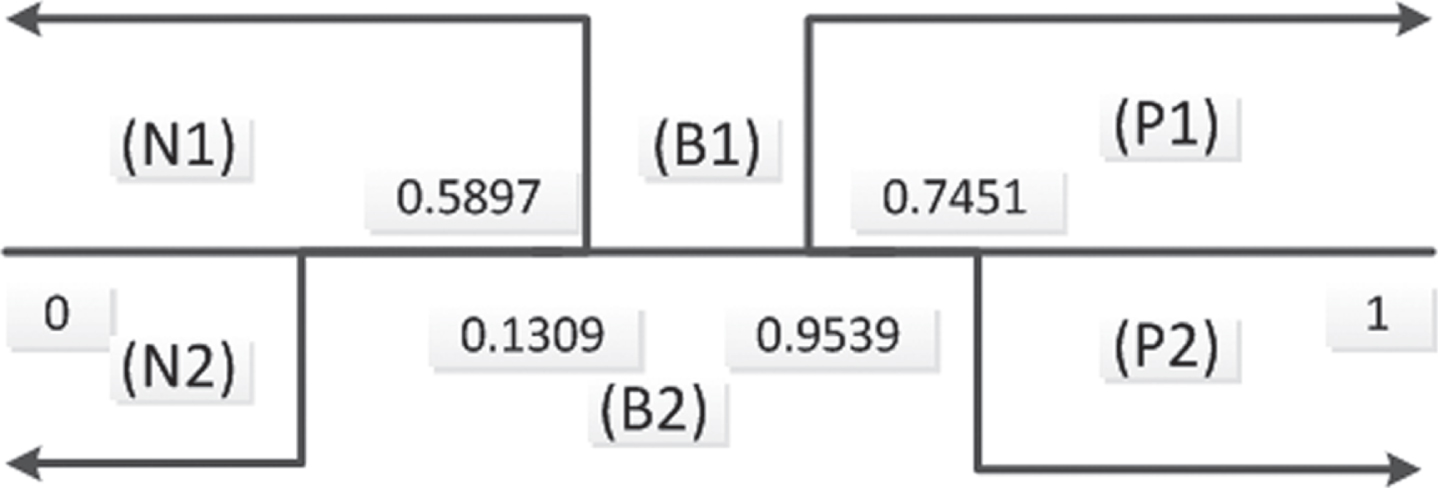
With the aid of Method 1, thresholds (α1, β1, γ1) of (P1) - (N1) are calculated using (25)-(27): α1 = 0.7451, β1 = 0.5897, γ1 = 0.7359. Thus, (P1) - (N1) are simply expressed as:
(P1) If , decide χ ∈ POS (D);
(B1) If , decide χ ∈ BND (D);
(N1) If , decide χ ∈ NEG (D).
Analogously, with the aid of Method 2, thresholds (α2, β2, γ2) of (P2) - (N2) are calculated using (28)-(30): α1 = 0.9539, β1 = 0.1309, γ1 = 0.3769. Thus, (P2) - (N2) are expressed as:
(P2) If , decide χ ∈ POS (D);
(B2) If , decide χ ∈ BND (D);
(N2) If , decide χ ∈ NEG (D).
In addition, in order to more clearly describe inconsistencies between (P1) - (N1) and (P2) - (N2), we visualized these decision rules in Fig. 2.
The inconsistency between (P1) - (N1) and (P2) - (N2).
From Fig. 2, we can find that decision rules (P1) - (N1) and (P2) - (N2) are asymmetric. Therefore, when we only use these rules to make decisions, these results obtained may be inconsistent.
Based on results in Example 5.1, Proposition 5.1 is the premise for Method 1 and 2 to obtain consistent decision results. That is to say, decision rules derived from Method 1 and Method 2 can be used only when Proposition 5.1 is true.
Method 3-5: Based on composite viewpoint
To solve the problem raised in Section 5.2, we need to synchronously consider the MD and the NMD of q-ROFNs. We introduce three different functions that compare the size of q-ROFNs to compare expected losses . The first is score and accuracy functions [14], the second is closeness index, and the third one is a new score function, which is defined in Ref [53]. Next, we will introduce these three methods respectively.
Method 3
According to Definition 2.4, score functions and accuracy functions of expected losses are calculated as formulas (31)-(36).
For (P), the condition implies the following prerequisites:
(E1) or
(E2) ;
In the same way, prerequisites for the second condition of rule (P) are:
(E3) or
(E4) ;
For the rule (B), we have:
(E5) or
(E6) ;
(E7) or
(E8) ;
And for the rule (N), we have:
(E9) or
(E10) ;
(E11) or
(E12) .
Therefore, decision rules (P) - (N) are expressed as (P3) - (N3):
According to Definition 2.6, these closeness indexes of expected losses are calculated as formulas (37)-(39).
Therefore, (P) - (N) are expressed as (P4) - (N4):
(P4) If and , decide χ ∈ POS (D);
(B4) If and , decide χ ∈ BND (D);
(N4) If and , decide χ ∈ NEG (D).
Method 5
According to Definition 2.7, These new score functions of expected losses are calculated as formulas (40)-(42).
Therefore, (P) - (N) are expressed as (P5) - (N5):
(P5) If and , decide χ ∈ POS (D);
(B5) If and , decide χ ∈ BND (D);
(N5) If and , decide χ ∈ NEG (D).
An algorithm to deduce TWDs for the MADM
We present an algorithm based on TWDs with q-ROFCDTRSs as follows:
Algorithm for the MADM with q-ROFCDTRSs
Input Decision-making table with q-ROF information and the loss function matrix with q-ROFNs;
Output Decision results;
Step 1. Calculate q-ROF β-neighborhood and q-RO β-neighborhood by using Definitions 3.1 and 3.2;
Step 2. By using the formula (9), we calculate the conditional probability .
Step 3. Give the loss function matrix with q-ROFNs, and calculate these values of thresholds (α1, β1, γ1) and (α2, β2, γ2) according to formulas (25)-(30), respectively.
Step 4. Calculate expected losses by using formulas (22) - (24). According to formulas (31)-(42), we acquire these values of score functions , accuracy functions , closeness indexes and new score functions with respect to expected losses respectively.
Step 5. Based on those five methods proposed in Section 5, POS (D), BND (D) and NEG (D) are calculated by using corresponding decision rules, respectively.
Step 6. Obtain decision results.
An illustrative example
Here, we will use those five methods based on q-ROFCDTRS to solve the employment problem of new teachers in Universities. The employment problem of new teachers is cited from the reference [28]. Then, we will use the example to illustrate the principles and steps of the q-ROFCDTRS model.
University leaders need to select the most qualified and suitable people to fill the required position. The discrete alternative set is U = {χ1, χ2, ⋯ , χ10} and the set of evaluation criteria is Research productivity, Managerial skill, Impact on research community, Ability to work under pressure, Academic leadership qualities, Contribution to one University. (Please refer to Ref [28] for detailed description and definition of attribute set.)
Because of the hesitancy, imprecision and uncertainty of the selection problem, decision makers use q-ROFNs to evaluate each candidate teacher. Evaluation results are shown in Table 4.
q-ROFSs for
χ1
(0.98, 0.3)
(0.7, 0.4)
(0.8, 0.2)
(0.9, 0.1)
(0.7, 0.6)
(0.4, 0.3)
χ2
(0.9, 0.4)
(0.7, 0.8)
(0.7, 0.8)
(0.6, 0.3)
(0.65, 0.57)
(0.6, 0.2)
χ3
(0.8, 0.7)
(0.7, 0.2)
(0.95, 0.4)
(0.8, 0.4)
(0.5, 0.2)
(0.8, 0.3)
χ4
(0.8, 0.3)
(0.6, 0.3)
(0.7, 0.4)
(0.9, 0.2)
(0.8, 0.65)
(0.4, 0.2)
χ5
(0.5, 0.2)
(0.95, 0.4)
(0.8, 0.3)
(0.7, 0.1)
(0.6, 0.3)
(0.94, 0.33)
χ6
(0.65, 0.25)
(0.75, 0.49)
(0.3, 0.55)
(0.9, 0.27)
(0.62, 0.36)
(0.68, 0.58)
χ7
(0.35, 0.35)
(0.65, 0.15)
(0.78, 0.3)
(0.64, 0.4)
(0.2, 0.55)
(0.8, 0.28)
χ8
(0.25, 0.48)
(0.5, 0.59)
(0.48, 0.28)
(0.57, 0.67)
(0.65, 0.4)
(0.9, 0.3)
χ9
(0.58, 0.4)
(0.65, 0.56)
(0.7, 0.24)
(0.4, 0.33)
(0.65, 0.58)
(0.25, 0.6)
χ10
(0.75, 0.4)
(0.85, 0.56)
(0.5, 0.35)
(0.63, 0.48)
(0.76, 0.2)
(0.66, 0.37)
Here we take the threshold β = (0.55, 0.69), we can get that is an q-ROF β-covering. Then , , , , , , , , , .
According to Definition 3.1, we can obtain the q-ROF β-neighborhood as shown in Table 5.
The q-ROF β-neighborhood
χ1
χ2
χ3
χ4
χ5
χ6
χ7
χ8
χ9
χ10
(0.7, 0.6)
(0.6, 0.8)
(0.5, 0.7)
(0.6, 0.65)
(0.5, 0.4)
(0.3, 0.55)
(0.2, 0.55)
(0.25, 0.67)
(0.4, 0.58)
(0.5, 0.56)
(0.4, 0.6)
(0.6, 0.57)
(0.5, 0.7)
(0.4, 0.65)
(0.5, 0.33)
(0.62, 0.58)
(0.2, 0.55)
(0.25, 0.67)
(0.25, 0.6)
(0.63, 0.48)
(0.4, 0.4)
(0.6, 0.8)
(0.7, 0.4)
(0.4, 0.4)
(0.7, 0.4)
(0.3, 0.58)
(0.64, 0.4)
(0.48, 0.67)
(0.25, 0.6)
(0.5, 0.56)
(0.7, 0.6)
(0.6, 0.8)
(0.5, 0.7)
(0.6, 0.65)
(0.5, 0.4)
(0.3, 0.55)
(0.2, 0.55)
(0.25, 0.67)
(0.4, 0.58)
(0.5, 0.56)
(0.4, 0.6)
(0.6, 0.8)
(0.5, 0.4)
(0.4, 0.65)
(0.6, 0.4)
(0.3, 0.58)
(0.2, 0.55)
(0.48, 0.67)
(0.25, 0.6)
(0.5, 0.56)
(0.4, 0.6)
(0.6, 0.8)
(0.5, 0.7)
(0.4, 0.65)
(0.5, 0.4)
(0.62, 0.58)
(0.2, 0.55)
(0.25, 0.67)
(0.25, 0.6)
(0.63, 0.56)
(0.4, 0.4)
(0.6, 0.8)
(0.7, 0.4)
(0.4, 0.4)
(0.7, 0.4)
(0.3, 0.58)
(0.64, 0.4)
(0.48, 0.67)
(0.25, 0.6)
(0.5, 0.56)
(0.4, 0.6)
(0.6, 0.57)
(0.5, 0.4)
(0.4, 0.65)
(0.6, 0.33)
(0.62, 0.58)
(0.2, 0.55)
(0.57, 0.67)
(0.25, 0.6)
(0.63, 0.48)
(0.7, 0.6)
(0.65, 0.8)
(0.5, 0.7)
(0.6, 0.65)
(0.5, 0.4)
(0.3, 0.55)
(0.2, 0.55)
(0.25, 0.59)
(0.58, 0.58)
(0.5, 0.56)
(0.4, 0.6)
(0.6, 0.8)
(0.5, 0.7)
(0.4, 0.65)
(0.5, 0.4)
(0.62, 0.58)
(0.2, 0.55)
(0.25, 0.67)
(0.25, 0.6)
(0.63, 0.56)
Based on Table 5 and formula (8), we have , , , , , , , , , .
Let the state set D = {χ3, χ5, χ6, χ9}. By formula (9), we have , , , , , , , , , .
Assume that the loss function matrix are shown as Table 6.
The loss function matrix 4
D
¬D
bP
T (λPP) = (0, 0.9)
T (λPN) = (0.85, 0.1)
bB
T (λBP) = (0.4, 0.5)
T (λBN) = (0.7, 0.3)
bN
T (λNP) = (0.85, 0.1)
T (λNN) = (0.02, 0.75)
Let , and . According to formulas (22)-(24) and Table 6, we can obtain expected losses as shown in Table 7.
Expected losses
RP (χ)
RB (χ)
RN (χ)
χ1
(0.85, 0.1)
(0.7, 0.3)
(0.02, 0.75)
χ2
(0.7775, 0.208)
(0.6388, 0.3557)
(0.6479, 0.3832)
χ3
(0.6478, 0.4326)
(0.5519, 0.4217)
(0.7774, 0.1957)
χ4
(0.85, 0.1)
(0.7, 0.3)
(0.85, 0.1)
χ5
(0, 0.9)
(0.4, 0.5)
(0.02, 0.75)
χ6
(0.7235, 0.3)
(0.5998, 0.3872)
(0.7235, 0.2738)
χ7
(0.6478, 0.4326)
(0.5519, 0.4217)
(0.7774, 0.1957)
χ8
(0.7578, 0.2408)
(0.624, 0.368)
(0.6816, 0.3349)
χ9
(0.7774, 0.208)
(0.6388, 0.3556)
(0.6479, 0.3831)
χ10
(0.7235, 0.3)
(0.5998, 0.3872)
(0.7235, 0.2738)
Next, we will use above five methods to solve the employment problem.
Decision results based on Method 1
Based on formulas (25)-(27), we calculate three thresholds α1, β1, γ1, respectively. Concretely, α1 = 0.8895, β1 = 0.3216, γ1 = 0.4999. According to the Method 1 and (P1) - (N1), we can get POS (D) = {χ5}, BND (D) = {χ2, χ3, χ6, χ7, χ8, χ9, χ10}, NEG (D) = {χ1, χ4}.
Decision results based on Method 2
Based on formulas (28)-(30), we calculate three thresholds α2, β2, γ2, respectively. Concretely, α2 = 0.6515, β2 = 0.3628, γ2 = 0.4784. According to the Method 2 and (P2) - (N2), we can get POS (D) = {χ3, χ5, χ7}, BND (D) = {χ6, χ8, χ10}, NEG (D) = {χ1, χ2, χ4, χ9}.
Decision results based on Method 3
Let , and . Based on the Method 3, according to the Table 7 and formulas (31)-(36), we can get score and accuracy functions of expected losses. These results are shown in Table 8.
Score and accuracy functions of expected losses
S (RP (χ))
S (RB (χ))
S (RN (χ))
H (RP (χ))
H (RB (χ))
H (RN (χ))
χ1
0.6131
0.316
-0.4218
0.6151
0.37
0.4218
χ2
0.4609
0.2157
0.2157
0.4789
0.3057
0.3282
χ3
0.1909
0.0931
0.4624
0.3529
0.2431
0.4774
χ4
0.6131
0.316
-0.4218
0.6151
0.37
0.4218
χ5
-0.729
-0.061
0.6131
0.729
0.189
0.6151
χ6
0.3518
0.1577
0.3582
0.4058
0.2739
0.3993
χ7
0.1909
0.0931
0.4624
0.3529
0.2431
0.4774
χ8
0.4212
0.1932
0.2791
0.4492
0.2929
0.3543
χ9
0.4609
0.2157
0.2157
0.4789
0.3057
0.3282
χ10
0.3518
0.1577
0.3582
0.4058
0.2739
0.3993
Based on (P3) - (N3), we can get POS (D) = {χ5}, BND (D) = {χ3, χ6, χ7, χ8, χ10}, NEG (D) = {χ1, χ2, χ4, χ9}.
Decision results based on Method 4
Let , and . Based on the Method 4, according to the Table 7 and formulas (37)-(39), we can get these closeness indexes of expected losses, respectively. Those results are shown in Table 9.
Closeness indexes
ϑ (RP (χ))
ϑ (RB (χ))
ϑ (RN (χ))
χ1
0.8065
0.658
0.2891
χ2
0.7304
0.6078
0.6078
χ3
0.5954
0.5465
0.7312
χ4
0.8065
0.658
0.2891
χ5
0.1355
0.4695
0.8065
χ6
0.6759
0.5788
0.6791
χ7
0.5954
0.5465
0.7312
χ8
0.7106
0.5966
0.6395
χ9
0.7304
0.6078
0.6078
χ10
0.6759
0.5788
0.6791
Therefore, Based on (P4) - (N4), we have POS (D) = {χ5}, BND (D) = {χ3, χ6, χ7, χ8, χ10}, NEG (D) = {χ1, χ2, χ4, χ9}.
Decision results based on Method 5
Let , and . Based on the Method 5, according to the Table 7 and formula (40)-(42), we calculate new score functions of expected losses. Those results are shown as Table 10.
New score functions
δ (RP (χ))
δ (RB (χ))
δ (RN (χ))
χ1
0.6217
0.5543
0.4025
χ2
0.5835
0.5367
0.5352
χ3
0.5296
0.5161
0.5848
χ4
0.6217
0.5543
0.4025
χ5
0.3396
0.4882
0.6217
χ6
0.5594
0.5269
0.5623
χ7
0.5296
0.5161
0.5848
χ8
0.5744
0.5328
0.5467
χ9
0.5835
0.5367
0.5352
χ10
0.5594
0.5269
0.5623
Therefore, according to (P4) - (N4), we have POS (D) = {χ5}, BND (D) = {χ3, χ6, χ7, χ8, χ10}, NEG (D) = {χ1, χ2, χ4, χ9}.
Comparisons and analyses
Next, we will compare and analyze the sensitivity of each parameter and the stability and effectiveness of these five methods proposed in Section 5.
Firstly, when β = (0.55, 0.69), q = 3. Decision results of MADM will vary with the vary of the loss function matrix. Suppose that there are four different loss function matrixes as shown in Table 6 and Tables11-13. Decision results are shown in Tables 14, which are obtained by five methods under different loss function matrixes.
The loss function matrix 1
D
¬D
bP
T (λPP) = (0.3, 0.7)
T (λPN) = (0.7, 0.2)
bB
T (λBP) = (0.5, 0.6)
T (λBN) = (0.3, 0.4)
bN
T (λNP) = (0.6, 0.2)
T (λNN) = (0.2, 0.5)
The loss function matrix 2
D
¬D
bP
T (λPP) = (0.3, 0.7)
T (λPN) = (0.6, 0.4)
bB
T (λBP) = (0.3, 0.6)
T (λBN) = (0.4, 0.7)
bN
T (λNP) = (0.7, 0.4)
T (λNN) = (0.1, 0.6)
The loss function matrix 3
D
¬D
bP
T (λPP) = (0.4, 0.7)
T (λPN) = (0.8, 0.2)
bB
T (λBP) = (0.5, 0.5)
T (λBN) = (0.6, 0.6)
bN
T (λNP) = (0.8, 0.3)
T (λNN) = (0.2, 0.8)
Comparison of decision results of five decision methods
Based on these five different loss function matrixes described in Tables11-13 and the Table 6, we use those five methods to obtain different decision results as shown in Table 14.
As shown in Table 14, based on the loss function matrix 1, decision results obtained by these 5 methods are the same; Based on the loss function matrix 2, decision results of Method 1 and Method 5 are the same, and decision results of Method 2, Method 3 and Method 4 are the same; Based on the loss function matrix 3, decision results of other four methods are the same except Method 2; Based on the loss function matrix 4, decision results of Method 1 and Method 2 are different from each other, and decision results of other three methods are the same. In all decision results, except when the loss function matrix is the loss function matrix 4, the positive domain POS (D) of Method 2 is {χ3, χ5, χ7}, the positive domain POS (D) of all other decision results is {χ5}. It can be seen from all decision results that when the loss function matrix is the same, decision results of Method 3 and Method 4 are the same. As mentioned before, based on Methods 3-5, expected losses are described by MD and NMD for q-ROFNs to obtain decision rules. However, according to Method 1, expected losses are characterized by the MD of q-ROFNs, and according to Method 2, expected losses are characterized by the NMD of q-ROFNs. Therefore, decision results obtained based on Methods 3-5 are more reasonable than those obtained by Methods 1 and 2.
{ Secondly, in order to illustrate the effectiveness and superiority of the model and methods presented in this paper, we use these 5 methods to calculate the example of Ref [57], and compare calculation results with those results of Ref [57], Comparison results are shown in Table 15. Here, we let q = 2.
Comparison of decision results with results of Ref. [57]
We can see from Table 15 that these decision results obtained by those methods are consistent, indicating that these 5 methods are correct and effective.
Thirdly, we will discuss the influence of each parameter on decision-making results when it changes independently.
(1) By considering the example in Section 6, when β = (0.55, 0.69) is kept unchanged and the value of q = i, i = 3, 4, ⋯ , 8 changes. Decision results are exactly the same as Table 14. It can be inferred that the value of the parameter q has no influence on decision results.
(2) By considering the above illustrative example in Section 6, when q = 3 is kept unchanged and the value of β changes. Here we use the loss function matrix 3 as the loss function matrix. When parameter β changes, decision results change, which are shown in Table 16.
The influence of parameter β changes.
β
Method
POS (D)
BND (D)
NEG (D)
Method 1
{χ3, χ5, χ6}
{χ1, χ2, χ4, χ7, χ8, χ9, χ10}
∅
β = (0.5, 0.5)
Method 2
{χ3, χ5, χ6}
{χ7, χ8, χ9, χ10}
{χ1, χ2, χ4}
Method 3
{χ3, χ5, χ6}
{χ1, χ2, χ4, χ7, χ8, χ9, χ10}
∅
Method 4
{χ3, χ5, χ6}
{χ1, χ2, χ4, χ7, χ8, χ9, χ10}
∅
Method 5
{χ3, χ5, χ6}
{χ1, χ2, χ4, χ7, χ8, χ9, χ10}
∅
Method 1
{χ3, χ5}
{χ1, χ6, χ9, χ10}
{χ2, χ4, χ7, χ8}
β = (0.5, 0.3)
Method 2
{χ3, χ5}
{χ1, χ6, χ9, χ10}
{χ2, χ4, χ7, χ8}
Method 3
{χ3, χ5}
{χ1, χ6, χ9, χ10}
{χ2, χ4, χ7, χ8}
Method 4
{χ3, χ5}
{χ1, χ6, χ9, χ10}
{χ2, χ4, χ7, χ8}
Method 5
{χ3, χ5}
{χ1, χ6, χ9, χ10}
{χ2, χ4, χ7, χ8}
Method 1
{χ5}
{χ2, χ3, χ6, χ7, χ8, χ9, χ10}
{χ1, χ4}
β = (0.55, 0.69)
Method 2
{χ5}
{χ3, χ6, χ7, χ8, χ10}
{χ1, χ2, χ4, χ9}
Method 3
{y5}
{χ2, χ3, χ6, χ7, χ8, χ9, χ10}
{χ1, χ4}
Method 4
{χ5}
{χ2, χ3, χ6, χ7, χ8, χ9, χ10}
{χ1, χ4}
Method 5
{χ5}
{χ2, χ3, χ6, χ7, χ8, χ9, χ10}
{χ1, χ4}
Method 1
{χ3, χ5}
{χ4, χ6, χ7, χ8, χ9, χ10}
{χ1, χ2}
β = (0.5, 0.2)
Method 2
{χ3, χ5}
{χ6, χ7, χ8, χ9, χ10}
{χ1, χ2, χ4}
Method 3
{χ3, χ5}
{χ4, χ6, χ7, χ8, χ9, χ10}
{χ1, χ2}
Method 4
{χ3, χ5}
{χ4, χ6, χ7, χ8, χ9, χ10}
{χ1, χ2}
Method 5
{χ3, χ5}
{χ4, χ6, χ7, χ8, χ9, χ10}
{χ1, χ2}
Method 1
{χ3, χ5χ3, χ5}
{χχ6, χ9, χ10}
{χ1, χ2, χ4, χ7, χ8}
β = (0.3, 0.3)
Method 2
{χ3, χ5}
{χ6, χ9, χ10}
{χ1, χ2, χ4, χ7, χ8}
Method 3
{χ3, χ5}
{χ6, χ9, χ10}
{χ1, χ2, χ4, χ7, χ8}
Method 4
{χ3, χ5}
{χ6, χ9, χ10}
{χ1, χ2, χ4, χ7, χ8}
Method 5
{χ3, χ5}
{χ6, χ9, χ10}
{χ1, χ2, χ4, χ7, χ8}
Method 1
{χ3, χ5}
{χ6, χ9, χ10}
{χ1, χ2, χ4, χ7, χ8}
β = (0.2, 0.3)
Method 2
{χ3, χ5}
{χ6, χ9, χ10}
{χ1, χ2, χ4, χ7, χ8}
Method 3
{χ3, χ5}
{χ6, χ9, χ10}
{χ1, χ2, χ4, χ7, χ8}
Method 4
{χ3, χ5}
{χ6, χ9, χ10}
{χ1, χ2, χ4, χ7, χ8}
Method 5
{χ3, χ5}
{χ6, χ9, χ10}
{χ1, χ2, χ4, χ7, χ8}
We can obtain from Table 16 that when the parameter β is determined, results obtained by those five methods are basically the same. When the parameter β is different, decision results have a small change. From Table 16, we can obtain that the value of the parameter β has a certain influence on decision results, and decision makers can select the appropriate parameter value β according to his preference.
Conclusions
We combined loss function matrix of DTRSs with Cq-ROFSs under the q-ROF environment in this paper. We proposed the q-ROFCDTRS model and elaborated its relevant properties. We established five methods to address expected losses expressed in the form of q-ROFNs, then derived these corresponding TWDs. Then, based on q-ROFCDTRS, we presented an algorithm for MADM problem. The conclusion of comparative analysis shows that these five methods proposed in this paper are effective and correct. Among them, Methods 3-5 have wider application range and better stability. Some advantages of the model and methods presented in this paper are as follows:
(1) The generalized distance calculation formula based on q-ROFNs is introduced, and the closeness index of q-ROFNs is proposed based on this distance. These provide a new method for distance calculation of q-ROFNs.
(2) Based on q-ROF β-neighborhood, the concept of q-RO β-neighborhood is proposed, and the conditional probability calculation method of q-ROFCAS is further given. These provide a new method for conditional probability calculation of q-ROFCAS.
(3) Aiming at the new uncertainty measure of q-ROFS, the loss function matrix of DTRS is discussed by using q-ROFNs. we construct an q-ROFCDTRS according to the Bayesian decision procedure, and put forward decision rules. These provide new ideas for using TWDs to solve MADM problems in the q-ROF environment.
In following research, we will focus on extending q-ROFCDTRS to consensus-based or social network based group decision making [58, 59].
Conflict of interest
The authors declare that they have no conflict of interest.
Footnotes
Acknowledgments
This research was funded by Sichuan Province Youth Science and Technology Innovation Team (Grant no.2019JDTD0015); Scientific Research Project of Department of Education of Sichuan Province (Grant no.18ZA0273, Grant no.15TD0027); Scientific Research Project of Neijiang Normal University (Grant no.18TD08). The Application Basic Research Plan Project of Sichuan Province (No. 2021JY0108).
References
1.
AtanassovK.T., Intuitionistic fuzzy sets, Fuzzy Sets and Systems20 (1986), 87–96.
2.
YagerR.R. and AbbasovA.M., Pythagorean Membership Grades, Complex Numbers, and Decision Making, International Journal of Intelligent Systems28(5) (2013), 436–452.
YagerR.R. and AlajlanN., Approximate reasoning with generalized orthopair fuzzy sets, Information Fusion38 (2017), 65–73.
5.
LuJ., HeT., WeiG., WuJ. and WeiC., Cumulative Prospect Theory: Performance Evaluation of Government Purchases of Home-Based Elderly-Care Services Using the Pythagorean 2-tuple Linguistic TODIM Method, International Journal of Environmental Research and Public Health17(6) (2020).
6.
GaoH., RanL.G., WeiG.W., WeiC. and WuJ., VIKOR Method for MAGDM Based on Q-Rung Interval-Valued Orthopair Fuzzy Information and Its Application to Supplier Selection of Medical Consumption Products, International Journal of Environmental Research and Public Health17(2) (2020).
7.
WeiG.W., WeiC., WuJ. and WangH.J., Supplier Selection of Medical Consumption Products with a Probabilistic Linguistic MABAC Method, International Journal of Environmental Research and Public Health16(24) (2019).
8.
WangJ., WangP., WeiG.W., WeiC. and WuJ., Some power Heronian mean operators in multiple attribute decision-making based on q-rung orthopair hesitant fuzzy environment, Journal of Experimental and Theoretical Artificial Intelligence (2019). doi:10.1080/0952813X.2019.1694592
9.
WangJ., WeiG.W., WangR., AlsaadiF.E., HayatT., WeiC., ZhangY. and WuJ., Some q-rung interval-valued orthopair fuzzy Maclaurin symmetric mean operators and their applications to multiple attribute group decision making, International Journal of Intelligent Systems34 (2019), 2769–2806.
10.
WangJ., WeiG.W., LuJ.P., AlsaadiF.E., HayatT., WeiC. and ZhangY., Some q-rung orthopair fuzzy Hamy mean operators in multiple attribute decision-making and their application to enterprise resource planning systems selection, International Journal of Intelligent Systems34 (2019), 2429–2458.
11.
WangJ., WeiG.W., WeiC. and WeiY., MABAC method for multiple attribute group decision making under q-rung orthopair fuzzy environment, Defence Technology16 (2020), 208–216.
12.
YagerR.R., AlajlanN. and BaziY., Aspects of generalized orthopair fuzzy sets, International Journal of Intelligent Systems33(11) (2018), 2154–2174.
13.
DuW.S., Minkowski-type distance measures for generalized orthopair fuzzy sets, International Journal of Intelligent Systems33(4) (2018), 802–817.
14.
LiuP. and LiuJ., Some q-rung orthopai fuzzy Bonferroni mean operators and their application to multi-attribute group decision making, International Journal of Intelligent Systems33(2) (2018), 315–347.
15.
LiangD.C. and CaoW., q-Rung orthopair fuzzy sets-based decision-theoretic rough sets for three-way decisions under group decision making, International Journal of Intelligent Systems34 (2019), 3139–3167.
16.
ZakowskiW., Approximations in the space (U, π), Demon and stration Mathematica16 (1983), 761–769.
17.
ZhanJ.M. and XuW.H., Two types of coverings based multi granulation rough fuzzy sets and applications to decision making, Artificial Intelligence Review53 (2020), 167–198.
18.
ZhanJ.M. and SunB.Z., Covering-based intuitionistic fuzzy rough sets and applications in multi-attribute decision-making, Artificial Intelligence Review53 (2020), 671–701.
19.
ZhanJ.M., ZhangX.H. and YaoY.Y., Covering based multigranulation fuzzy rough sets and corresponding applications, Artificial Intelligence Review53 (2020), 1093–1126.
20.
ZhangK., ZhanJ.M. and WuW.Z., Novel fuzzy rough set models and corresponding applications to multi-criteria decisionmaking, Fuzzy Sets and Systems383 (2020), 92–126.
21.
ZhangL., ZhanJ.M. and YaoY.Y., Intuitionistic fuzzy TOPSIS method based on CVPIFRS models: An application to biomedical problems, Information Sciences517 (2020), 315–339.
22.
JiangH.B., ZhanJ.M., SunB.Z. and AlcantudJ.C.R., An MADM approach to covering-based variable precision fuzzy rough sets: an application to medical diagnosis, International Journal of Machine Learning and Cybernetics11 (2020), 2181–2207.
23.
ZhangZ., KouX.Y., YuW.Y. and GaoY., Consistency improvement for fuzzy preference relations with selfconfidence: An application in two-sided matching decision making, Journal of the Operational Research Society (2020). doi:10.1080/01605682.2020.1748529
24.
ZhangZ., YuW., MartinezL. and GaoY., Managing Multigranular Unbalanced Hesitant Fuzzy Linguistic Information in Multiattribute Large-Scale Group Decision Making: A Linguistic Distribution-Based Approach, IEEE Transactions on Fuzzy Systems (2019), dio:10.1109/TFUZZ.2019.2949758
25.
MaL.W., Two fuzzy covering rough set models and their generalizations over fuzzy lattices, Fuzzy Sets and Systems294 (2016), 1–17.
26.
DąŕeerL., RestrepoM., CornelisC., GĺőmezJ., Neighborhood operators for covering-based rough sets, Information Sciences336 (2016), 21–44.
27.
DąŕeerL., CornelisC., GodoL., Fuzzy neighborhood operators based on fuzzy coverings, Fuzzy Sets and Systems312 (2017), 17–35.
28.
HussainA., IrfanA. M. and MahmoodT., Covering based q-rung orthopair fuzzy rough set model hybrid with TOPSIS for multi-attribute decision making, Journal of Intelligent and Fuzzy Systems37(1) (2019), 981–993.
29.
JiaX.Y., LiaoW.H., TangZ.M. and ShangL., Minimum cost attribute reduction in decision-theoretic rough set models, Information Sciences219 (2013), 151–167.
30.
LiH.X., ZhouX.Z., ZhaoJ.B. and LiuD., Attribute reduction in decision-theoretic rough set model: a further investigation, International Conference on Rough Sets and Knowledge Technology, Berlin, Heidelberg: Springer (2011), 466–475.
31.
MinF. and ZhuW., Attribute reduction of data with error ranges and test costs, Information Sciences211 (2012), 48–67.
32.
YaoY. and ZhaoY., Attribute reduction in decision-theoretic rough set models, Information Sciences178(17) (2008), 3356–3373.
33.
ZhaoY., WongS.K.M. and YaoY.Y., A note on attribute reduction in the decision-theoretic rough set model, Transactions on Rough Sets XIII. Berlin, Heidelberg: Springer (2011), 260–275.
34.
LiangD.C., LiuD., PedryczW. and HuP., Triangular fuzzy decision-theoretic rough sets, International Journal of Approximate Reasoning54(8) (2013), 1087–1106.
35.
LiuD., LiT.R. and RuanD., Probabilistic model criteria with decision-theoretic rough sets, Information Sciences181(17) (2011), 3709–3722.
36.
DengX.F. and YaoY.Y., Decision-theoretic three-way approximations of fuzzy sets, Information Sciences279 (2014), 702–715.
37.
LiW.T. and XuW.H., Double-quantitative decision-theoretic rough set, Information Sciences316 (2015), 54–67.
38.
LiangD.C. and LiuD., Systematic studies on three-way decisions with interval-valued decision-theoretic rough sets, Information Sciences276 (2014), 186–203.
39.
YuH., ZhangC. and WangG.Y., A tree-based incremental overlapping clustering method using the three-way decision theory, Knowledge-Based Systems91 (2016), 189–203.
40.
YuH. and WangY., Three-way decisions method for overlapping clustering, International Conference on Rough Sets and Current Trends in Computing, Berlin, Heidelberg, Springer (2012), 277–286.
41.
LiuD., LiT.R. and LiangD.C., Three-way government decision analysis with decision-theoretic rough sets, Int J Uncertain Fuzz Knowl-based Syst20(1) (2012), 119–132.
42.
ChenY., YueX., FujitaH., et al., Three-way decision support for diagnosis on focal liver lesions, Knowl-Based Syst127 (2017), 85–99.
43.
LiuD., YaoY.Y. and LiT.R., Three-way investment decisions with decision-theoretic rough sets, Int J Comput Intell Syst4 (2011), 66–74.
44.
LiangD.C., PedryczW., LiuD. and HuP., Three-way decisions based on decision-theoretic rough sets under linguistic assessment with the aid of group decision making, Applied Soft Computing29 (2015), 256–269.
45.
YaoY. and ZhouB., Naive Bayesian rough sets, International Conference on Rough Set and Knowledge TechnologySpringer-Verlag (2010), 719–726.
46.
LiuD., LiT.R. and LiangD.C., Incorporating logistic regression to decision-theoretic rough sets for classifications, International Journal Approximate Reasoning55 (2014), 197–210.
47.
LiangD.C. and LiuD., A novel risk decision making based on decision-theoretic rough sets under hesitant fuzzy information, IEEE Transactions on Fuzzy Systems23(2) (2015), 237–247.
48.
LiangD.C. and LiuD., Deriving three-way decisions from intuitionistic fuzzy decision-theoretic rough sets, Information Sciences300 (2015), 28–48.
49.
MandalP. and RanadiveA.S., Decision-theoretic rough sets under Pythagorean fuzzy information, International Journal of Intelligent Systems33 (2018), 1–18.
50.
GaoJ., LiangZ.L., ShangJ. and XuZ.S., Continuities, Derivatives and Differentials of q-Rung Orthopair Fuzzy Functions, IEEE Transactions on Fuzzy Systems27(8) (2018), 1687–1699.
51.
LiuF., WuJ., MouL. and LiuY., Decision Support Methodology Based on Covering-Based Interval-Valued Pythagorean Fuzzy Rough Set Model and Its Application to Hospital Open-Source EHRs System Selection, Mathematical Problems in Engineering2020 (2020), 1–13.
52.
HwangC.L. and YoonK.S., Multiple Attribute Decision Methods and Applications, Springer, Berlin Heidelberg (1981).
53.
LiH.X., YinS.Y. and YangY., Some preference relations based on q-rung orthopair fuzzy sets, International Journal of Intelligent Systems34(11) (2019), 2920–2936.
54.
YaoY.Y. and WongS.K.M., A decision theoretic framework for approximating concepts, International Journal of Man-Machine Studies37(6) (1992), 793–809.
55.
YaoY.Y., Three-way decisions with probabilistic rough sets, Information Sciences180(3) (2010), 341–353.
56.
ChenT.Y., Bivariate models of optimism and pessimism in multi-criteria decision-making based on intuitionistic fuzzy sets, Information Sciences181(11) (2011), 2139–2165.
57.
ZhangH.D. and MaQ., Three-way decisions with decisiontheoretic rough sets based on Pythagorean fuzzy covering, Soft Computing18 (2020), doi: 10.1007/s00500-070-05102-4.
58.
YuW.Y., ZhangZ. and ZhongQ.Y., Consensus reaching for MAGDMwith multi-granular hesitant fuzzy linguistic term sets: a minimum adjustment-based approach, Annals of Operations Research (2019), doi:10.1007/s10479-019-03432-7
59.
ZhangZ., GaoY. and LiZ.L., Consensus reaching for social network group decision making by considering leadership and bounded confidence, Knowledge-Based Systems204 (2020). doi: 10.1016/j.knosys.2020.106240.