Necessary and sufficient conditions for existence of solutions for initial value problem of fuzzy Bagley-Torvik equation and solution representation

Abstract

In this paper, we investigate the necessary and sufficient conditions for existence of solutions for initial value problem of fuzzy Bagley-Torvik equation and the solution representation by using the multivariate Mittag-Leffler function. First we convert fuzzy initial value problem into the cut problem (system of fractional differential equations with inequality constraints) and obtain existence results for the solution of the cut problem under (1,1)- differentiability. Next we study the conditions for the solutions of the cut problem to constitute the solution of a fuzzy initial value problem and suggest a necessary and sufficient condition for the (1,1)-solution. Also, some examples are given to verify the effectiveness of our proposed method. The necessary and sufficient condition, solution representation for (1,2)-solution of initial value problem of fuzzy fractional Bagley-Torvik equation are shown in Appendix.

Keywords

Fuzzy Fuzzy Bagley-Torvik equation generalized Hukuhara differentiability multivariate Mittag-Leffler function

1 Introduction

As fractional differential equations (FDEs) play the important roles in modeling the real world, such as physics, chemistry, biology, viscous flow, acoustics, electromagnetic flow, economics, and so on, many researchers have focused on FDEs.

In [8], Bagley and Torvik modeled the motion of large and thin plates moving in Newtonian liquids by the initial value problem of the following fractional differential equations. $\begin{matrix} y^{″} (t) + b \cdot D^{1.5} y (t) + c \cdot y (t) = f (t), t \in (0, 1], \\ y (0) = y_{0}, y^{'} (0) = y_{0}^{'} . \end{matrix}$ Thereafter numerical methods for the Bagley-Torvik equation have been extensively studied. The scientists obtained numerical solutions of the Bagley-Torvik equations by using generalized Taylor collocation method, hybridizable discontinuous Galerkin methods, hybrid functions approximation, fractional Legendre collocation method, fractional neural network model, Haar wavelet operation matrix method, Adomian decomposition method, discrete spline method, etc. ([5 , 27– 30]).

Other hand, the uniqueness and existence of the positive solution for the boundary value problem of the generalized Bagley-Torvik equation using the Leray-Schauder principle was studied in [25] and the existence of solution for the Neumann problem of the generalized Bagley-Torvik equation was considered in [26].

As the real-world is modeled by the initial value problem of the differential equation, the initial conditions and the parameters of the equation can usually be uncertainty

Therefore, many researchers have considered the existence of solution and numerical methods for fuzzy differential equations. ([2 , 31– 33]).

In [37], the concreted solutions of the fuzzy linear fractional differential equations with the fuzzy initial condition under Riemann-Liouville-differentiability have been studied and in [38], the method for find exact fuzzy solution of the fuzzy wave-like equations in one and two dimensions have been introduced.

Also the concept of Caputo fuzzy type fractional derivative in the case of the order α ∈ (1, 2) has been introduced in [12] and the existence and uniqueness of solution for an initial value problem of fuzzy fractional differential equations has been studied.

The fuzzy fractional Volterra integro-differential equation in [34] and fuzzy fractional differential equation in [35] have been introduced in case which fractional order is 0 < β ≤ 1. First they have converted the proposed problems into the system of ordinary fractional differential equations and revealed the numerical method to solve the system of ordinary fractional differential equations, obtained the numerical results for r-cut function of (1)-solution and (2)-solution.

Currently, there are few results for the fuzzy Bagley-Torvik equation and we could not find the results except in [10]. In [10], they obtained the numerical solution of (1,1)-solution for following fuzzy fractional Bagley-Torvik equation by using homotopy perturbation method. $\begin{matrix} a \otimes y^{″} (t) \oplus b \otimes^{c} D^{1.5} y (t) \oplus c \otimes y (t) = f (t), \\ y (0) = y_{0}, y^{'} (0) = y_{0}^{'}, t \in (0, 1] . \end{matrix}$

However, they did not consider the fact that the existence of a solution for the initial value problem of constant coefficient fuzzy linear differential equations depends on the coefficients, initial values and non-homogeneous terms.(see Example 5.1.)

In contrast to the crisp case, for fuzzy fractional differential equations the existence of a solution is not fully clarified even for the constant coefficient linear case, which can be said to be a theoretical gap.

In [14], they have noted that in general a solution of a fractional fuzzy integral equation is not a solution of a fractional fuzzy differential equation.

In other words, the traditional approach used in crisp fractional differential equations cannot be applied. Therefore, the study of the existence of solutions of fuzzy fractional differential equations requires a new method.

The aim of this paper is to propose a new method for the existence of solutions of fuzzy fractional differential equations and to fill the gaps on the uniqueness and existence of the solutions.

In this paper, we investigate the uniqueness and existence of the solution for the initial value problem of the fuzzy Bagley-Torvik equation $D_{n, m}^{(2)} y (t) \oplus b \otimes^{c} D_{n, m}^{β} y (t) \oplus c \otimes y (t) = f (t),$ (1) $y (0) = y_{0}, D_{n}^{(1)} y (0) = y_{0}^{'}, t \in (0, 1],$ (2) where $1 < β < 2, b, c \in R_{+}, y_{0}, y_{0}^{'} \in R_{F}, y, f \in C (J, R_{F}), n, m \in {1, 2}, J = [0, 1]$ .

We obtain a cut problem with inequality constraints corresponding to the fuzzy initial value problem Definition 2.3and a necessary and sufficient condition for the existence of a (1,1)-solution of the fuzzy Bagley-Torvik equation by using the solution of cut problem. Also we suggest the representation of (1,1)-solution. Next the results of (1,2)-solution are considered.

We think that our method are applicable to general types of constant coefficient fractional fuzzy linear differential equations.

Our paper organized as follows. We introduce the basic concepts and some results used in this paper in Section 2. Section 3 are proposed the necessary and sufficient condition for the existence of a (1,1)-solution of the fuzzy fractional Bagley-Torvik equation. By using multivariate Mittag-Leffler function, the representation of (1,1)-solution of the fuzzy fractional Bagley-Torvik equation is suggested in Section4. Through several examples, we evaluate the effectiveness of our method in Section 5. Conclusions are given in Section 6 and the results for (1,2)-solution are shown in Appendix.

2 Preliminaries

Definition 2.1 [4] A fuzzy number is a function u : R → [0, 1] satisfying the following properties:

i) u is normal,

ii) u is a convex fuzzy set,

iii) u is upper semi-continuous,

iv) The set $\bar{Supp (u)}$ is compact on R (where Supp (u) : = {x ∈ R|u (x) >0}).

Denote the set of fuzzy numbers R_F.

For u, v, w ∈ R_F, if there exists w ∈ R_F such that u = v ⊕ w, then w is called the H-difference of u and v, and it is denoted by w : = u ⊖ _Hv.

Definition 2.2. [20] Let y : (a, b) → R_F and t₀ ∈ (a, b).

i) We say that y is (1)-differentiable at t₀, if there exists an element y′ (t₀) ∈ R_F such that for all h > 0 sufficiently small, ∃y (t₀ + h) ⊖ _Hy (t₀), y (t₀) ⊖ _Hy (t₀ - h) and the limits $\begin{matrix} y^{'} (t_{0}) = \\ lim_{h \to 0^{+}} \frac{y (t_{0} + h) ⊖_{H} y (t_{0})}{h} = lim_{h \to 0^{+}} \frac{y (t_{0}) ⊖_{H} y (t_{0} - h)}{h} \end{matrix}$ exist.

ii) We say that y is (2)-differentiable at t₀, if there exists an element y′ (t₀) ∈ R_F such that for all h > 0 sufficiently small, ∃y (t₀) ⊖ _Hy (t₀ + h), y (t₀ - h) ⊖ _Hy (t₀) and limits $\begin{matrix} y^{'} (t_{0}) = \\ lim_{h \to 0^{+}} \frac{y (t_{0}) ⊖_{H} y (t_{0} + h)}{- h} = lim_{h \to 0^{+}} \frac{y (t_{0} - h) ⊖_{H} y (t_{0})}{- h} \end{matrix}$ exist.

When y is (1)-differentiable or (2)-differentiable at t₀, y′ (t₀) is denoted by $D_{1}^{(1)} y (t_{0})$ or $D_{2}^{(1)} y (t_{0})$ .

Definition 2.3. [1] Let y : (a, b) → R_F, t₀ ∈ (a, b). If there exists $D_{m}^{(1)} (D_{n}^{(1)} y) (t_{0})$ for $D_{n}^{(1)} y (t_{0})$ , we say that y is (n, m)-differentiable and $D_{m}^{(1)} (D_{n}^{(1)} y)$ (t₀) is denoted by $D_{n, m}^{(2)} y (t_{0})$ , where n, m ∈ {1, 2} .

Definition 2.4. [20] Let y : (a, b) → R_F, β ≥ 0. Then $I_{0 +}^{β} y (t) : = {\begin{matrix} \frac{1}{Γ (β)} \int_{0}^{t} (t - s)^{β - 1} y (s) ds, & β > 0, \\ y (t), & β = 0 \end{matrix}$ is called fuzzy Riemann-Liouville fractional integral of order β of y.

Lemma 2.1 [20] Let y : (a, b) → R_F, [y (t)] ^r : = [y₁ (t, r) , y₂ (t, r)]. Then $[I_{0 +}^{β} y (t)]^{r} = [I_{0 +}^{β} y_{1} (t, r), I_{0 +}^{β} y_{2} (t, r)], 0 \leq r \leq 1 .$

Definition 2.5. Let y : (a, b) → R_F be a fuzzy function such that $\begin{matrix} G_{1} (t) : = & \frac{1}{Γ (2 - β)} \int_{0}^{t} (t - s)^{1 - β} \otimes \\ (y (s) \underset{H}{⊖} (y (0) \oplus s \otimes D_{1}^{(1)} y (0))) ds \end{matrix}$ exists. Then, the fuzzy Caputo fractional derivatives of order β of y is defined as follows: $^{c} D_{1, n}^{β} y (t) : = D_{1, n}^{(2)} G_{1} (t), n \in {1, 2}$ .

We say that y is ^c [(1, n) - β]-differentiable if there exist $^{c} D_{1, n}^{β} y (t),$ n ∈ {1, 2} .

Definition 2.6. [15] For u ∈ R_F and r ∈ (0, 1], denote [u] ^r = {t ∈ R|u (t) ≥ r}. We call this set an r-cut of the fuzzy number u.

Lemma 2.2. Let y : (a, b) → R_F, 1 < β < 2 and [y (t)] ^r : = [y₁ (t, r) , y₂ (t, r)]. Then

i) If y is ^c [(1, 1) - β]-differentiable,

$[^{c} D_{1, 1}^{β} y (t)]^{r} = [^{c} D_{0 +}^{β} y_{1} (t, r),^{c} D_{0 +}^{β} y_{2} (t, r)]$ ,

ii) If y is ^c [(1, 2) - β]-differentiable,

$[^{c} D_{1, 2}^{β} y (t)]^{r} = [^{c} D_{0 +}^{β} y_{2} (t, r),^{c} D_{0 +}^{β} y_{1} (t, r)]$ .

Proof. First we prove i) of Lemma 2.2 when y is ^c [(1, 1) - β]-differentiable. From Definition 2.5, $^{c} D_{1, 1}^{β} y (t) = D_{1, 1}^{(2)} G_{1} (t)$ . Let [G₁ (t)] ^r = [G_1,1 (t, r) , G_1,1 (t, r)]. Then from [39], $[D_{1, 1}^{(2)} G_{1} (t)]^{r} = [G_{1, 1}^{″} (t, r), G_{1, 2}^{″} (t, r)]$ holds.

Also let $[y (s)]^{r} = [y_{1} (s, r), y_{2} (s, r)], [y (0)]^{r} = [y_{0, 1} (r), y_{0, 2} (r)], [D_{1}^{(1)} y (0)]^{r} = [y_{0, 1}^{'} (r), y_{0, 2}^{'} (r)]$ . If $y (s) \underset{H}{⊖} (y (0) \oplus s \otimes D_{1}^{(1)} y (0))$ exists, then $\begin{matrix} G_{1, 1}^{″} (t, r) = & \frac{1}{Γ (2 - β)} \frac{d^{2}}{{dt}^{2}} \int_{0}^{t} (t - s)^{1 - β} \cdot \\ (y_{1} (s, r) - y_{0, 1} (r) - {sy}_{0, 1}^{'} (r)) ds \end{matrix}$ $\begin{matrix} G_{1, 2}^{″} (t, r) = & \frac{1}{Γ (2 - β)} \frac{d^{2}}{{dt}^{2}} \int_{0}^{t} (t - s)^{1 - β} \cdot \\ (y_{2} (s, r) - y_{0, 2} (r) - {sy}_{0, 2}^{'} (r)) ds . \end{matrix}$ Therefore, we get $[^{c} D_{1, 1}^{β} y (t)]^{r} = [^{c} D_{0 +}^{β} y_{1} (t, r),^{c} D_{0 +}^{β} y_{2} (t, r)] .$ We proved for case i) of the Lemma 2.2 when y is ^c [(1, 1) - β]-differentiable. For the case which y is ^c [(1, 2) - β]-differentiable, the proof is similar to the above one.

Lemma 2.3. [9] Let {U_r|r ∈ [0, 1]} be a family of real intervals such that the following three conditions are satisfied

i) For all r ∈ [0, 1], U_r is a non-empty compact interval,

ii) If 0 < α < β ≤ 1, then U_β ⊆ U_α,

iii) For given any non-decreasing sequence r_n ∈ (0, 1] with $lim_{n \to \infty} r_{n} = r$ , $U_{r} = ⋂_{n = 1}^{\infty} U_{r_{n}}$ .

Then there exists a unique fuzzy number u ∈ R_F such that [u] ^r = U_r for all r ∈ (0, 1] and [u] ⁰ = cl (⋃ _r∈(0,1]U_r).

Definition 2.7. [3] Let u ∈ R_F, r ∈ [0, 1] , [u] ^r = [u₁, u₂]. Then the diameter of a fuzzy number u is defined by d ([u] ^r) : = u₂ - u₁.

In paper, we promise the following symbols. For f : (a, b) → R_F, [f (t)] ^r : = [f₁ (t, r) , f₂ (t, r)] , $\begin{matrix} Δ_{(r_{1}, r_{2})} f_{1} (t) : = f_{1} (t, r_{2}) - f_{1} (t, r_{1}), \\ Δ_{(r_{1}, r_{2})} f_{2} (t) : = f_{2} (t, r_{2}) - f_{2} (t, r_{1}) . \end{matrix}$

3 Necessary and sufficient condition for the existence of solution for initial value problem of fuzzy Bagley-Torvik type equation

Definition 3.1. We say that y (t) is (n, m)-solution of the initial value problem (1), (2) if y ∈ C (J, R_F) satisfies (1), (2) and $\begin{matrix} D_{n, m}^{(2)} y \in C (J, R_{F}),^{c} D_{n, m}^{β} y \in C (J, R_{F}), \\ D_{n}^{(1)} y \in C (J, R_{F}) . \end{matrix}$ C (J, R_F) is a space of fuzzy-valued functions, which are continuous on J. In this section, we consider the existence of the (1,1)-solution of the following initial value problem: $D_{1, 1}^{(2)} y (t) \oplus b \otimes^{c} D_{1, 1}^{β} y (t) \oplus c \otimes y (t) = f (t),$ (3) $y (0) = y_{0}, D_{1}^{(1)} y (0) = y_{0}^{'}, t \in (0, 1]$ (4) where $1 < β < 2, b, c \in R_{+}, y_{0}, y_{0}^{'} \in R_{F}, y, f \in C (J, R_{F}), J = [0, 1] .$

First of all, we consider the fractional integral equation: $U (t) + p (t) I_{0 +}^{λ_{1}} U (t) + q (t) I_{0 +}^{λ_{2}} U (t) = V (t), t \in J,$ (5) where V, p, q ∈ C (J) , λ₁, λ₂ > 0.

Lemma 3.1. The integral equation (5) has a unique solution U (t) in C (J) and the solution U (t) satisfies the following inequality ${∥ U ∥}_{C (J)} \leq \frac{e^{k_{*}}}{1 - M} {∥ V ∥}_{C (J)},$ where k_* is a positive number with $M : = (\frac{| | p | |_{C (J)}}{k_{*}^{λ_{1}}} +$ $\frac{| | q | |_{C (J)}}{k_{*}^{λ_{2}}}) < 1$ and || · ||_C(J) is max-norm on C (J).

Proof. Let denote $F (U) (t) : = V (t) - p (t) I_{0 +}^{λ_{1}} U (t) - q (t) I_{0 +}^{λ_{2}} U (t)$ , equation (5) present as follows $U (t) = F (U) (t) .$ We discuss by using following k-norm equivalent with max-norm in C (J) ${∥ x ∥}_{k} : = max {e^{- kt} | x (t) |}, x \in C (J) .$ For X, Y ∈ C (J), we get $\begin{matrix} | F (X) (t) - F (Y) (t) | \leq | | p | |_{C (I)} {∥ X (t) - Y (t) ∥}_{k} \cdot \\ \cdot I_{0 +}^{λ_{1}} e^{kt} + | | q | |_{C (I)} {∥ X (t) - Y (t) ∥}_{k} I_{0 +}^{λ_{2}} e^{kt} \end{matrix}$ Estimating $I_{0 +}^{λ_{1}} e^{kt}, k > 0$ in above right side, from definition of fractional integral and Gamma function, we obtain $\begin{matrix} I_{0 +}^{λ_{1}} e^{kt} = & \frac{e^{kt}}{Γ (λ_{1}) \cdot k^{λ_{1}}} \cdot \int_{0}^{kt} s^{λ_{1} - 1} e^{- s} ds \\ \leq \frac{e^{kt}}{Γ (λ_{1})} \cdot k^{λ_{1}} \cdot \int_{0}^{\infty} s^{λ_{1} - 1} e^{- s} ds = \frac{e^{kt}}{k^{λ_{1}}} . \end{matrix}$ $\begin{array}{l} I_{0 +}^{λ_{1}} e^{k t} = & \frac{e^{k t}}{Γ (λ_{1}) \cdot k^{λ_{1}}} \cdot \int_{0}^{k t} s^{λ_{1} - 1} e^{- s} d s \\ \leq \frac{e^{k t}}{Γ (λ_{1})} \cdot k^{λ_{1}} \cdot \int_{0}^{\infty} s^{λ_{1} - 1} e^{- s} d s = \frac{e^{k t}}{k^{λ_{1}}} . \end{array}$ Similarity $I_{0 +}^{λ_{2}} e^{kt} \leq \frac{e^{kt}}{k^{λ_{2}}}$ . That is, for ∀X, Y ∈ C (J), it holds $\begin{matrix} e^{- kt} & | F (X) (t) - F (Y) (t) | \\ \leq (\frac{| | p | |_{C (J)}}{k^{λ_{1}}} + \frac{| | q | |_{C (J)}}{k^{λ_{2}}}) | | X - Y | |_{k}, \end{matrix}$ therefore we have $\begin{matrix} | | F_{1} (X) - F_{1} (Y) | |_{k} \\ \leq (\frac{| | p | |_{C (J)}}{k^{λ_{1}}} + \frac{| | q | |_{C (J)}}{k^{λ_{2}}}) | | X - Y | |_{k} . \end{matrix}$ By choosing a constant $k_{*} > 0$ satisfying $M : = (\frac{| | p | |_{C (J)}}{k_{*}^{λ_{1}}} + \frac{| | q | |_{C (J)}}{k_{*}^{λ_{2}}}) < 1,$ the following fact holds $| | F (X) - F (Y) | |_{k_{*}} \leq M | | X - Y | |_{k_{*}} .$ From the completeness of C (J), the equivalent of max-norm and $k_{*}$ -norm, we get $\exists \bar{Y} \in C (J); \bar{Y} = F (\bar{Y}) .$ So the integral equation (5) has a unique solution U = U (t) in C (J).

Now let proceed upper estimate of solution. Because U (t) is the solution of Eq. (5), we have $| U (t) | \leq ∥ p ∥ I_{0 +}^{λ_{1}} | U (t) | + ∥ q ∥ I_{0 +}^{λ_{2}} | U (t) | + | V (t) |,$ $\begin{matrix} {∥ U ∥}_{k} & \leq ∥ p ∥ \frac{1}{k^{λ_{1}}} {∥ U ∥}_{k} + ∥ q ∥ \frac{1}{k^{λ_{2}}} {∥ U ∥}_{k} + {∥ V ∥}_{k} \\ = (∥ p ∥ \frac{1}{k^{λ_{1}}} + ∥ q ∥ \frac{1}{k^{λ_{2}}}) {∥ U ∥}_{k} + {∥ V ∥}_{k} . \end{matrix}$ By choosing a constant $k_{*} > 0$ in the same way as above, the following inequality holds. $\begin{matrix} {∥ U ∥}_{k_{*}} \leq \frac{1}{1 - M} {∥ V ∥}_{k_{*}}, \\ e^{- k_{*}} {∥ U ∥}_{C (J)} \leq {∥ U ∥}_{k_{*}} \leq \frac{{∥ V ∥}_{k_{*}}}{1 - M} \leq \frac{{∥ V ∥}_{C (J)}}{1 - M}, \\ {∥ U ∥}_{C (J)} \leq \frac{e^{k_{*}}}{1 - M} {∥ V ∥}_{C (J)} . \end{matrix}$ □

The cut equation of (3) is as follows for r ∈ [0, 1]: $[D_{1, 1}^{(2)} y (t) \oplus b \otimes^{c} D_{1, 1}^{β} y (t) \oplus c \otimes y (t)]^{r} = [f (t)]^{r} .$

Based on the operation of the intervals, we can rewrite this equation as follows: $[D_{1, 1}^{(2)} y (t) (t)]^{r} + b [^{c} D_{1, 1}^{β} y (t)]^{r} + c [y (t)]^{r} = [f (t)]^{r} .$ (6)

Using [y (t)] ^r : = [y₁ (t, r) , y₂ (t, r)] and (iii) of Lemma 2.2, cuts of $D_{1, 1}^{(2)} y (t),^{c} D_{1, 1}^{β} y (t)$ are as follows: $\begin{matrix} [D_{1, 1}^{(2)} y (t)]^{r} = [y_{1}^{″} (t, r), y_{2}^{″} (t, r)], \\ [^{c} D_{1, 1}^{β} y (t)]^{r} = [^{c} D_{0 +}^{β} y_{1} (t, r),^{c} D_{0 +}^{β} y_{2} (t, r)] . \end{matrix}$

Also using[f (t)] ^r : = [f₁ (t, r) , f₂ (t, r)], we obtain the following: $\begin{matrix} [y_{1}^{″} (t, & r), y_{2}^{″} (t, r)] + b [^{c} D_{0 +}^{β} y_{1} (t, r),^{c} D_{0 +}^{β} y_{2} (t, r)] \\ + c [y_{1} (t, r), y_{2} (t, r)] = [f_{1} (t, r), f_{2} (t, r)] . \end{matrix}$

Therefore, we obtain the cut-problem (7) corresponding to the problem (3) ${\begin{matrix} y_{1}^{″} (t, r) + b^{c} D_{0 +}^{β} y_{1} (t, r) + {cy}_{1} (t, r) = f_{1} (t, r), \\ y_{2}^{″} (t, r) + b^{c} D_{0 +}^{β} y_{2} (t, r) + {cy}_{2} (t, r) = f_{2} (t, r), \\ y_{1} (t, r) \leq y_{2} (t, r), \\ y_{1}^{'} (t, r) \leq y_{2}^{'} (t, r), \\ ^{c} D_{0 +}^{β} y_{1} (t, r) \leq^{c} D_{0 +}^{β} y_{2} (t, r), \\ y_{1}^{″} (t, r) \leq y_{2}^{″} (t, r) . \end{matrix}$ (7)

Let $[y_{0}]^{r} : = [y_{0, 1} (r), y_{0, 2} (r)], [y_{0}^{'}]^{r} : = [y_{0, 1}^{'} (r),$ $y_{0, 2}^{'} (r)]$ , then the initial conditions of (7) are as follows: $\begin{matrix} y_{1} (0, r) = y_{0, 1} (r), y_{1}^{'} (0, r) = y_{0, 1}^{'} (r), \\ y_{2} (0, r) = y_{0, 2} (r), y_{2}^{'} (0, r) = y_{0, 2}^{'} (r) . \end{matrix}$ (8)

Definition 3.2. We say that (y₁ (t, r) , y₂ (t, r)) is the solution of the cut-problem (7), (8) if y₁ (t, r) , y₂ (t, r) satisfies (7), (8) and $y_{1}^{″} (\cdot, r), y_{2}^{″} (\cdot, r) \in C (J)$ .

We introduce the following symbol: $Δ_{(r_{1}, r_{2})} f (t) = f (t, r_{2}) - f (t, r_{1}) .$

Theorem 3.1. (Necessary condition) Let y (t) be the (1,1)-solution of (3), (4) and its cut be [y (t)] ^r : = [y₁ (t, r) , y₂ (t, r)], then (y₁ (t, r) , y₂ (t, r)) is the solution of (7) and (8) and the following facts are true.

(C1) If The integral equation $\begin{matrix} U (t) + & {bI}_{0 +}^{2 - β} U (t) + {cI}_{0 +}^{2} U (t) \\ = d ([f (t)]^{r}) - c (d ([y_{0}]^{r}) + d ([y_{0}^{'}]^{r}) t) \end{matrix}$ has a unique solution U ∈ C (J).

(C2) If r₁, r₂ ∈ [0, 1] , r₁ ≤ r₂, $V_{1} (t) : = y_{1}^{″} (t, r_{2}) - y_{1}^{″} (t, r_{1})$ , then the integral equation $\begin{matrix} V_{1} & (t) + {bI}_{0 +}^{2 - β} V_{1} (t) + {cI}_{0 +}^{2} V_{1} (t) \\ = Δ_{(r_{1}, r_{2})} f_{1} (t) - c (Δ_{(r_{1}, r_{2})} y_{0, 1} + Δ_{(r_{1}, r_{2})} y_{0, 1}^{'} t) \end{matrix}$ has a unique non-negative solution V₁ ∈ C (J).

(C3) If r₁, r₂ ∈ [0, 1] , r₁ ≤ r₂, $V_{2} (t) : = y_{2}^{″} (t, r_{2}) - y_{2}^{″} (t, r_{1})$ then the integral equation $\begin{matrix} V_{2} & (t) + {bI}_{0 +}^{2 - β} V_{2} (t) + {cI}_{0 +}^{2} V_{2} (t) \\ = Δ_{(r_{1}, r_{2})} f_{2} (t) - c (Δ_{(r_{1}, r_{2})} y_{0, 2} + Δ_{(r_{1}, r_{2})} y_{0, 2}^{'} t) \end{matrix}$ has a unique non-positive solution V₂ ∈ C (J).

Proof. The fact that (y₁ (t, r) , y₂ (t, r)) is the solution of (7) and (8) is obvious by the definition.

Next, we prove (C1).

We obtain the following system of cut-equation: ${\begin{matrix} y_{1}^{″} (t, r) + b^{c} D_{0 +}^{β} y_{1} (t, r) + {cy}_{1} (t, r) = f_{1} (t, r), \\ y_{2}^{″} (t, r) + b^{c} D_{0 +}^{β} y_{2} (t, r) + {cy}_{2} (t, r) = f_{2} (t, r) \end{matrix}$ (9) and initial condition $\begin{matrix} y_{1} (0, r) = y_{0, 1} (r), y_{1}^{'} (0, r) = y_{0, 1}^{'} (r), \\ y_{2} (0, r) = y_{0, 2} (r), y_{2}^{'} (0, r) = y_{0, 2}^{'} (r) . \end{matrix}$ (10)

Denote $z_{1} (t, r) : = y_{1}^{″} (t, r), z_{2} (t, r) : = y_{1}^{″} (t, r),$ (11) then by the definition of the solution, z₁, z₂ ∈ C (J) and $z_{1} (t, r) \leq z_{2} (t, r) .$ (12)

Therefore, the following equations hold. $\begin{matrix} y_{1} (t, r) = I_{0 +}^{2} z_{1} (t, r) + y_{0, 1} (r) + t \cdot y_{0, 1}^{'} (r), \\ y_{2} (t, r) = I_{0 +}^{2} z_{2} (t, r) + y_{0, 2} (r) + t \cdot y_{0, 2}^{'} (r) . \end{matrix}$ (13)

Thus we obtain $\begin{matrix} ^{c} D_{0 +}^{β} y_{1} (t, r) = I_{0 +}^{2 - β} z_{1} (t, r), \\ ^{c} D_{0 +}^{β} y_{2} (t, r) = I_{0 +}^{2 - β} z_{2} (t, r) . \end{matrix}$ (14)

From (11), (13), (14), we obtain ${\begin{matrix} \begin{matrix} z_{1} (t, r) & + {bI}_{0 +}^{2 - β} z_{1} (t, r) + {cI}_{0 +}^{2} z_{1} (t, r) \\ = f_{1} (t, r) - c (y_{0, 1} (r) + y_{0, 1}^{'} (r) t), \end{matrix} \\ \begin{matrix} z_{2} (t, r) & + {bI}_{0 +}^{2 - β} z_{2} (t, r) + {cI}_{0 +}^{2} z_{2} (t, r) \\ = f_{2} (t, r) - c (y_{0, 2} (r) + y_{0, 2}^{'} (r) t) . \end{matrix} \end{matrix}$ Thus, we get $\begin{matrix} U (t) & + {bI}_{0 +}^{2 - β} U (t) + {cI}_{0 +}^{2} U (t) \\ = d ([f (t)]^{r}) - c (d ([y_{0}]^{r}) + d ([y_{0}^{'}]^{r}) t), \end{matrix}$ (15) where U (t) : = z₂ (t, r) - z₁ (t, r).

On the other hand, by the Lemma 3.1, the equation (33) has a unique solution and by (30), the solution of (33) is non-negative. Thus, (C1) is proved.

Next, we prove (C2).

Since $D_{1, 1}^{(2)} y \in C (J, R_{F})$ and $[D_{1, 1}^{(2)} y (t)]^{r} = [y_{1}^{″} (t, r), y_{2}^{″} (t, r)]$ , for the fixed t ∈ J, $y_{1}^{″} (t, r)$ is increasing with respect to r, $y_{2}^{″} (t, r)$ is decreasing with respect to r.

Thus, for any r₁, r₂ ∈ [0, 1] , r₁ ≤ r₂, the following inequalities hold: $y_{1}^{″} (t, r_{1}) \leq y_{1}^{″} (t, r_{2}),$ (16) $y_{2}^{″} (t, r_{1}) \geq y_{2}^{″} (t, r_{2}) .$ (17)

On the other hand, from the first equation in (9), we obtain the following system of differential equations: ${\begin{matrix} y_{1}^{″} (t, r_{1}) + b^{c} D_{0 +}^{β} y_{1} (t, r_{1}) + {cy}_{1} (t, r_{1}) = f_{1} (t, r_{1}), \\ y_{1}^{″} (t, r_{2}) + b^{c} D_{0 +}^{β} y_{1} (t, r_{2}) + {cy}_{1} (t, r_{2}) = f_{1} (t, r_{2}) . \end{matrix}$

Now, let us denote Δy₁ (t) : = y₁ (t, r₂) - y₁ (t, r₁). Then we get the following equation: $\begin{matrix} Δ_{(r_{1}, r_{2})} y_{1}^{″} (t) & + b^{c} D_{0 +}^{β} Δ_{(r_{1}, r_{2})} y_{1} (t) \\ + c Δ_{(r_{1}, r_{2})} y_{1} (t) = Δ_{(r_{1}, r_{2})} f_{1} (t) . \end{matrix}$ (18) Here, the initial condition of function Δ_(r₁,r₂)y₁ (t) is as follows: $\begin{matrix} Δ_{(r_{1}, r_{2})} y_{1} (0) = y_{1} (0, r_{2}) - y_{1} (0, r_{1}) = Δ_{(r_{1}, r_{2})} y_{0, 1}, \\ Δ_{(r_{1}, r_{2})} y_{1}^{'} (0) = y_{1}^{'} (0, r_{2}) - y_{1}^{'} (0, r_{1}) = Δ_{(r_{1}, r_{2})} y_{0, 1}^{'} . \end{matrix}$ (19) Let us denote $V_{1} (t) : = Δ_{(r_{1}, r_{2})} y_{1}^{″} (t)$ in the initial value problem (36), (37). Then we obtain the integral equation which is equivalent to (36): $\begin{matrix} V_{1} (t) & + {bI}_{0 +}^{2 - β} V_{1} (t) + {cI}_{0 +}^{2} V_{1} (t) \\ = Δ_{(r_{1}, r_{2})} f_{1} (t) - c (Δ_{(r_{1}, r_{2})} y_{0, 1} + Δ_{(r_{1}, r_{2})} y_{0, 1}^{'} t) \end{matrix}$

By Lemma 3.1, above integral equation has a unique solution and from (34), V₁ (t) ≥0, t ∈ J. Thus, (C2) is proved. In a similar manner to above proof, we can prove (C3). This completes the proof of the Theorem 3.1. □

Now, let us consider the sufficient conditions for the existence of (1,1)-solution of fuzzy initial value problem (3) and (4).

Lemma 3.2. Let $(y_{1} (t, r), y_{2} (t, r))$ be the solution of (7) and (8). Then $(φ_{1} (t, r), φ_{2} (t, r))$ given by $φ_{1} (t, r) : = y_{1}^{″} (t, r), φ_{2} (t, r) : = y_{2}^{″} (t, r)$ is the solution of following problem: ${\begin{matrix} \begin{matrix} φ_{1} (t, r) & + {bI}_{0 +}^{2 - β} φ_{1} (t, r) + {cI}_{0 +}^{2} φ_{1} (t, r) \\ = f_{1} (t, r) - c (y_{0, 1} (r) + y_{0, 1}^{'} (r) t), \end{matrix} \\ \begin{matrix} φ_{2} (t, r) & + {bI}_{0 +}^{2 - β} φ_{2} (t, r) + {cI}_{0 +}^{2} φ_{2} (t, r) \\ = f_{2} (t, r) - c (y_{0, 2} (r) + y_{0, 2}^{'} (r) t), \end{matrix} \\ φ_{1} (t, r) \leq φ_{2} (t, r) \end{matrix}$ (20) in C (J). Conversely, if $(φ_{1} (t, r), φ_{2} (t, r))$ is the solution of problem (38), then $(y_{1} (t, r), y_{2} (t, r))$ given by $\begin{matrix} y_{1} (t, r) = y_{0, 1} (r) + y_{0, 1}^{'} (r) t + I_{0 +}^{2} φ_{1} (t, r), \\ y_{2} (t, r) = y_{0, 2} (r) + y_{0, 2}^{'} (r) t + I_{0 +}^{2} φ_{2} (t, r) \end{matrix}$ (21) is the solution of cut-problem (7), (8).

Lemma 3.2 can be easily proved by transforming (9) into integral equation considering its initial condition (10).

The existence and uniqueness of solution of the integral equations in (38) are guaranteed by Lemma 3.1. Now let us consider the sufficient condition for the unique solution to satisfy the inequality in (38).

Lemma 3.3. If the integral equation $\begin{matrix} U (t) & + {bI}_{0 +}^{2 - β} U (t) + {cI}_{0 +}^{2} U (t) \\ = d ([f (t)]^{r}) - c (d ([y_{0}]^{r}) + d ([y_{0}^{'}]^{r}) t) \end{matrix}$ has a non-negative solution U ∈ C (J), then $φ_{1} (t, r) \leq φ_{2} (t, r)$ holds.

Proof. By the Lemma 3.1, above integral equation has unique solution. Therefore, by the assumption-U ∈ C (J) is non-negative, we can see that $φ_{1} (t, r) \leq φ_{2} (t, r)$ . □

By above consideration, we can draw the conclusions that if b, c ∈ R₊, f ∈ C (I, R_F) and the function $d ([f (t)]^{r}) - c (d ([y_{0}]^{r}) + d ([y_{0}^{'}]^{r}) t)$ satisfies the assumption of Lemma 3.3, then the problem (38) has a unique solution. Therefore, the cut-problem (7), (8) has a unique solution.

By Lemma 3.2 and Lemma 3.3, we obtain the following inequalities: $y_{1}^{″} (t, r) \leq y_{2}^{″} (t, r), t \in J, r \in [0, 1],$ (22) $y_{1} (t, r) \leq y_{2} (t, r), t \in I, r \in [0, 1],$ (23) $^{c} D_{0 +}^{β} y_{1} (t, r) \leq^{c} D_{0 +}^{β} y_{2} (t, r), t \in I, r \in [0, 1] .$ (24)

Also, using (39) and (40), we have $y_{1}^{'} (t, r) \leq y_{2}^{'} (t, r), t \in I, r \in [0, 1] .$ (25)

Hence, the intervals are valid:

$\begin{matrix} {U_{2} (t, r) : = [y_{1}^{″} (t, r), y_{2}^{″} (t, r)], r \in [0, 1]}, \\ {U_{β} (t, r) : = [^{c} D_{0 +}^{β} y_{1} (t, r),^{c} D_{0 +}^{β} y_{2} (t, r)], r \in [0, 1]}, \\ {U_{1} (t, r) : = [y_{1}^{'} (t, r), y_{2}^{'} (t, r)], r \in [0, 1]}, \\ {U_{0} (t, r) : = [y_{1} (t, r), y_{2} (t, r)], r \in [0, 1]} . \end{matrix}$

Now, we will prove that the above families of intervals constitute fuzzy valued functions.

Theorem 3.2. Suppose that the following two assumptions are satisfied:

i) Let r₁, r₂ ∈ [0, 1] , r₁ ≤ r₂. Then the integral equation $\begin{matrix} U (t) + {bI}_{0 +}^{2 - β} U (t) + {cI}_{0 +}^{2} U (t) \\ = Δ_{(r_{1}, r_{2})} f_{1} (t) - c (Δ_{(r_{1}, r_{2})} y_{0, 1} + Δ_{(r_{1}, r_{2})} y_{0, 1}^{'} t) \end{matrix}$ has a unique non-negative solution U ∈ C (J).

ii) Let r₁, r₂ ∈ [0, 1] , r₁ ≤ r₂. Then the integral equation $\begin{matrix} U (t) + {bI}_{0 +}^{2 - β} U (t) + {cI}_{0 +}^{2} U (t) \\ = Δ_{(r_{1}, r_{2})} f_{2} (t) - c (Δ_{(r_{1}, r_{2})} y_{0, 2} + Δ_{(r_{1}, r_{2})} y_{0, 2}^{'} t) \end{matrix}$ has a unique non-positive solution U ∈ C (J).

Then the families of the intervals $\begin{matrix} {U_{2} (t, r), r \in [0, 1]}, {U_{β} (t, r), r \in [0, 1]}, \\ {U_{1} (t, r), r \in [0, 1]}, {U_{0} (t, r), r \in [0, 1]} \end{matrix}$ constitute fuzzy valued functions.

Proof. It is sufficient to prove that the families of the intervals satisfy the second and third condition of Lemma 2.3. First, let us prove that {U₂ (t, r) , r ∈ [0, 1]} satisfies the second condition of Lemma 2.3.

For fixed r₁, r₂ ∈ [0, 1] (0 < r₁ < r₂ ≤ 1), denote as $\begin{matrix} Δ_{(r_{1}, r_{2})} φ_{1} (t) : = φ_{1} (t, r_{2}) - φ_{1} (t, r_{1}), \\ Δ_{(r_{1}, r_{2})} φ_{2} (t) : = φ_{2} (t, r_{2}) - φ_{2} (t, r_{1}) . \end{matrix}$

Using the first equation of (38), we have

$\begin{matrix} Δ_{(r_{1}, r_{2})} φ_{1} (t) + {bI}_{0 +}^{2 - β} Δ_{(r_{1}, r_{2})} φ_{1} (t) + {cI}_{0 +}^{2} Δ_{(r_{1}, r_{2})} φ_{1} (t) \\ = Δ_{(r_{1}, r_{2})} f_{1} (t) - c (Δ_{(r_{1}, r_{2})} y_{0, 1} + Δ_{(r_{1}, r_{2})} y_{0, 1}^{'} t), \end{matrix}$

and by Lemma 3.1 and assumption i), we have $Δ_{(r_{1}, r_{2})} φ_{1} (t) \geq 0, t \in J .$ (26)

That is, $y_{1}^{″} (t, r_{1}) \leq y_{1}^{″} (t, r_{2}) .$

Analogously, using the second equation of (38), we have the following equality: $\begin{matrix} Δ_{(r_{1}, r_{2})} φ_{2} (t) + {bI}_{0 +}^{2 - β} Δ_{(r_{1}, r_{2})} φ_{2} (t) + {cI}_{0 +}^{2} Δ_{(r_{1}, r_{2})} φ_{2} (t) \\ = Δ_{(r_{1}, r_{2})} f_{2} (t) - c (Δ_{(r_{1}, r_{2})} y_{0, 2} + Δ_{(r_{1}, r_{2})} y_{0, 2}^{'} t) \end{matrix}$ and by assumption ii), we get $Δ_{(r_{1}, r_{2})} φ_{2} (t) \leq 0, t \in J,$ (27) that is, $y_{2}^{″} (t, r_{2}) \leq y_{2}^{″} (t, r_{1}) .$

Therefore, the family of intervals {U₂ (t, r) : r ∈ [0, 1]} satisfies the second condition of the Lemma 2.3.

On the other hand, from the first equation of (39), we have the following equations:

$\begin{matrix} y_{1} (t, r_{2}) - y_{1} (t, r_{1}) \\ = Δ_{(r_{1}, r_{2})} y_{0, 1} + Δ_{(r_{1}, r_{2})} y_{0, 1}^{'} t + I_{0 +}^{2} Δ_{(r_{1}, r_{2})} φ_{1} (t), \\ y_{1}^{'} (t, r_{2}) - y_{1}^{'} (t, r_{1}) = Δ_{(r_{1}, r_{2})} y_{0, 1}^{'} + I_{0 +}^{1} Δ_{(r_{1}, r_{2})} φ_{1} (t), \\ ^{c} D_{0 +}^{β} y_{1} (t, r_{2}) -^{c} D_{0 +}^{β} y_{1} (t, r_{1}) = I_{0 +}^{2 - β} Δ_{(r_{1}, r_{2})} φ_{1} (t) . \end{matrix}$

From (26), we get the following inequalities. $\begin{matrix} y_{1} (t, r_{2}) - y_{1} (t, r_{1}) \geq 0, \\ y_{1}^{'} (t, r_{2}) - y_{1}^{'} (t, r_{1}) \geq 0, \\ ^{c} D_{0 +}^{β} y_{1} (t, r_{2}) -^{c} D_{0 +}^{β} y_{1} (t, r_{1}) \geq 0 . \end{matrix}$ (28)

Analogously, from the second equation of (39), we can get the following inequalities: $\begin{matrix} y_{2} (t, r_{2}) - y_{2} (t, r_{1}) \leq 0, \\ y_{2}^{'} (t, r_{2}) - y_{2}^{'} (t, r_{1}) \leq 0, \\ ^{c} D_{0 +}^{β} y_{2} (t, r_{2}) -^{c} D_{0 +}^{β} y_{2} (t, r_{1}) \leq 0 . \end{matrix}$ (29)

Thus, from (46), (47), we can see that the families of the intervals $\begin{matrix} {U_{β} (t, r) : r \in [0, 1]}, {U_{1} (t, r) : r \in [0, 1]}, \\ {U_{0} (t, r) : r \in [0, 1]} \end{matrix}$ also satisfy the second condition of the Lemma 2.3.

Next, let us prove that the families of the intervals satisfy the third condition of Lemma 2.3. In other words, we will prove that the following results hold for any non-decreasing sequence r_n ∈ (0, 1] with $lim_{n \to \infty} r_{n} = r$ . $\begin{matrix} lim_{n \to \infty} y_{1} (t, r_{n}) = y_{1} (t, r), lim_{n \to \infty} y_{2} (t, r_{n}) = y_{2} (t, r), \\ lim_{n \to \infty} y_{1}^{'} (t, r_{n}) = y_{1}^{'} (t, r), lim_{n \to \infty} y_{2}^{'} (t, r_{n}) = y_{2}^{'} (t, r), \\ lim_{n \to \infty}^{c} D_{0 +}^{β} y_{1} (t, r_{n}) =^{c} D_{0 +}^{β} y_{1} (t, r), \\ lim_{n \to \infty}^{c} D_{0 +}^{β} y_{2} (t, r_{n}) =^{c} D_{0 +}^{β} y_{2} (t, r), \\ lim_{n \to \infty} y_{1}^{″} (t, r_{n}) = y_{1}^{″} (t, r), lim_{n \to \infty} y_{2}^{″} (t, r_{n}) = y_{2}^{″} (t, r) . \end{matrix}$

Denote as $h (t, r_{n}, r) : = f_{1} (t, r_{n}) - f_{1} (t, r) - c ((y_{1} (0, r_{n}) - y_{1} (0, r)) + (y_{1}^{'} (0, r_{n}) - y_{1}^{'} (0, r)) t)$ . Then, using (38) we get $\begin{matrix} φ_{1} (t, r_{n}) & - φ_{1} (t, r) + {bI}_{0 +}^{2 - β} (φ_{1} (t, r_{n}) - φ_{1} (t, r)) \\ + {cI}_{0 +}^{2} (φ_{1} (t, r_{n}) - φ_{1} (t, r)) = h (t, r_{n}, r) . \end{matrix}$

By Lemma 3.1, there exists w > 0 such that $| | φ_{1} (\cdot, r_{n}) - φ_{1} (\cdot, r) | |_{C (J)} \leq w | | h (\cdot, r_{n}, r) | |_{C (J)} .$

By the left-hand continuity of $f_{1}, y_{1}, y_{1}^{'}$ with respect to variable r, we get $lim_{n \to \infty} h (t, r_{n}, r) = 0,$ (30) hence, $lim_{n \to \infty} φ_{1} (t, r_{n}) = φ_{1} (t, r),$ (31) that is, $lim_{n \to \infty} y_{1}^{″} (t, r_{n}) = y_{1}^{″} (t, r) .$

In the similar manner, we can prove $lim_{n \to \infty} y_{2}^{″} (t, r_{n}) = y_{2}^{″} (t, r)$ (32) holds.

From (21), (31) and (32), we get the followings: $\begin{matrix} lim_{n \to \infty} y_{1} (t, r_{n}) = y_{1} (t, r), lim_{n \to \infty} y_{2} (t, r_{n}) = y_{2} (t, r), \\ lim_{n \to \infty} y_{1}^{'} (t, r_{n}) = y_{1}^{'} (t, r), lim_{n \to \infty} y_{2}^{'} (t, r_{n}) = y_{2}^{'} (t, r), \\ lim_{n \to \infty}^{c} D_{0 +}^{β} y_{1} (t, r_{n}) =^{c} D_{0 +}^{β} y_{1} (t, r), \\ lim_{n \to \infty}^{c} D_{0 +}^{β} y_{2} (t, r_{n}) =^{c} D_{0 +}^{β} y_{2} (t, r) . \end{matrix}$

Therefore, the families of the intervals satisfy the third condition of the Lemma 2.3. □

Denote by ${\tilde{y}}_{2} (t), {\tilde{y}}_{β} (t), {\tilde{y}}_{1} (t), {\tilde{y}}_{0} (t)$ the fuzzy valued functions, which are constituted by the families of intervals ${U_{2} (t, r) : = [y_{1}^{″} (t, r), y_{2}^{″} (t, r)], r \in [0, 1],}$ (33) ${U_{β} (t, r) : = [^{c} D_{0 +}^{β} y_{1} (t, r),^{c} D_{0 +}^{β} y_{2} (t, r)], r \in [0, 1]},$ (34) ${U_{1} (t, r) : = [y_{1}^{'} (t, r), y_{2}^{'} (t, r)], r \in [0, 1]},$ (35) ${U_{0} (t, r) : = [y_{1} (t, r), y_{2} (t, r)], r \in [0, 1]} .$ (36)

Then the following result holds.

Theorem 3.3. Fuzzy valued functions ${\tilde{y}}_{2} (t),$ ${\tilde{y}}_{β} (t), {\tilde{y}}_{1} (t)$ and ${\tilde{y}}_{0} (t)$ are continuous on J.

Proof. First, Let us prove $lim_{t \to t_{*}} {\tilde{y}}_{2} (t) = {\tilde{y}}_{2} (t_{*})$ for any t_* ∈ J. Since $\begin{matrix} D ({\tilde{y}}_{2} (t), {\tilde{y}}_{2} (t_{*})) = sup_{r \in [0, 1]} max & {| y_{1}^{″} (t, r) - y_{1}^{″} (t_{*}, r) |, \\ | y_{2}^{″} (t, r) - y_{2}^{″} (t_{*}, r) |}, \end{matrix}$ it is sufficient to prove the continuity of $y_{1}^{″} (t, r), y_{2}^{″} (t, r)$ with respect to t. Since y₁ (t, r) , y₂ (t, r) are the solutions of (7) and (8), continuity of $y_{1}^{″} (t, r)$ and $y_{2}^{″} (t, r)$ with respect to t are guaranteed. Similarly, from (39), we can see that ${\tilde{y}}_{β} (t), {\tilde{y}}_{1} (t)$ and ${\tilde{y}}_{0} (t)$ are continuous. □

Lemma 3.4. For any t ∈ J, the following holds: $D_{1}^{(1)} {\tilde{y}}_{0} (t) = \tilde{y} (t), t \in J .$ (37)

It is obvious from the definition of (1)-derivative.

Theorem 3.4. The following relations hold: ${\tilde{y}}_{0} (t) = {\tilde{y}}_{0} (0) \oplus {\tilde{y}}_{1} (0) \otimes t \oplus I_{0 +}^{2} {\tilde{y}}_{2} (t)$ (38) ${\tilde{y}}_{β} (t) = I_{0 +}^{2 - β} {\tilde{y}}_{2} (t)$ (39) $D_{1, 1}^{(2)} {\tilde{y}}_{0} (t) = {\tilde{y}}_{2} (t)$ (40)

Proof. By the Theorem 3.3, ${\tilde{y}}_{2} (t)$ is continuous, hence $I_{0 +}^{2} {\tilde{y}}_{2} (t), I_{0 +}^{2 - β} {\tilde{y}}_{2} (t)$ is valid. From (39) and (51)-(54), we can get (56), (57). Now, let us prove (58).

By Lemma 3.4 and (56), (58) can be written as ${\tilde{y}}_{0} (t) = {\tilde{y}}_{0} (0) \oplus D_{1}^{(1)} {\tilde{y}}_{0} (0) \otimes t \oplus I_{0 +}^{2} {\tilde{y}}_{2} (t)$

Using the definition of H-difference, it can be rewritten as ${\tilde{y}}_{0} (t) ⊖_{H} ({\tilde{y}}_{0} (0) \oplus D_{1}^{(1)} {\tilde{y}}_{0} (0) \otimes t) = I_{0 +}^{2} {\tilde{y}}_{2} (t) .$

Thus, we obtain $^{c} D_{1, 1}^{(2)} {\tilde{y}}_{0} (t) = {\tilde{y}}_{2} (t) .$ □

Remark 3.1. From Theorem 3.4, we can see that ${\tilde{y}}_{0} (t)$ is the (1,1)-solution of (3), (4) in the sense of Definition 3.1. Therefore the following facts hold $D_{1, 1}^{(2)} y (t) = {\tilde{y}}_{2} (t),$ $^{c} D^{β} y (t) = {\tilde{y}}_{β} (t),$ $D_{1}^{(1)} y_{1} (t) = {\tilde{y}}_{1} (t),$ $y (t) = {\tilde{y}}_{0} (t)$

We can get the sufficient condition for the existence of solution for (3) and (4) from Theorem 3.2-3.4.

Theorem 3.5. (Sufficient condition) Suppose that (y₁ (t, r) , y₂ (t, r)) is the solution of (7) and (8) and (C1)-(C3) hold. Then the fuzzy initial value problem (3), (4) has a unique (1,1)-solution.

Based on Theorem 3.1 and Theorem 3.5, there exist solution to (7) and (8) and (C1)-(C3) hold.

4 Solution representation for initial value problem of fuzzy Bagley-Torvik equation

In this section, we study the solution representation for fuzzy initial value problem (3) and (4).

Theorem 4.1. ((1,1)-solution representation) (1,1)-solution representation for fuzzy initial value problem (3) and (4) is as follows:

$\begin{matrix} y (t) \\ = y_{0} \oplus t \otimes y_{0}^{'} \oplus y_{0} \otimes {ct}^{2} E_{(2 - β, 2), 3}^{-} ({bt}^{2 - β}, {ct}^{2}) \\ \oplus (y_{0}^{'} \otimes {ct}^{3} E_{(2 - β, 2), 4}^{+} ({bt}^{2 - β}, {ct}^{2}) \\ \oplus \int_{0}^{t} (t - s) E_{(2 - β, 2), 2}^{+} (b (t - s)^{2 - β}, c (t - s)^{2}) \otimes f (s) ds \\ ⊖_{H} (y_{0} \otimes {ct}^{2} E_{(2 - β, 2), 3}^{+} ({bt}^{2 - β}, {ct}^{2}) \\ \oplus y_{0}^{'} \otimes {ct}^{3} E_{(2 - β, 2), 4}^{-} ({bt}^{2 - β}, {ct}^{2}) \\ \oplus \int_{0}^{t} (t - s) E_{(2 - β, 2), 2}^{-} (b (t - s)^{2 - β}, c (t - s)^{2}) \otimes f (s) ds) \end{matrix}$

Proof. The solution of first equations of (7) and (8) represent as follows from [36] $\begin{matrix} y_{1} (t, r) = y_{0, 1} (r) + t \cdot y_{0, 1}^{'} (r) - c \cdot y_{0, 1} (r) \cdot t^{2} \\ \cdot E_{(2 - β, 2), 3} (- {bt}^{2 - β}, - {ct}^{2}) - c \cdot y_{0, 1}^{'} (r) \cdot t^{3} \\ \cdot E_{(2 - β, 2), 4} (- {bt}^{2 - β}, - {ct}^{2}) + \int_{0}^{t} (t - s) \\ \cdot E_{(2 - β, 2), 2} (- b (t - s)^{2 - β}, - c (t - s)^{2}) f_{1} (s, r) ds \end{matrix}$ (41)

On the other hand, we obtain the following facts for two variable Mittag-Leffler function $\begin{matrix} E_{(α_{1}, α_{2}), α_{3}} (- {ct}^{α_{1}}, - {bt}^{α_{2}}) \\ = \sum_{k = 0}^{\infty} \sum_{l_{1}, l_{2} \geq 0}^{l_{1} + l_{2} = k} (\begin{matrix} k \\ l_{1}, l_{2} \end{matrix}) \frac{(- {ct}^{α_{1}})^{l_{1}} (- {bt}^{α_{2}})^{l_{2}}}{Γ (b + α_{1} l_{1} + α_{2} l_{2})} \\ = \sum_{k = 0}^{\infty} (- 1)^{k} \sum_{l_{1}, l_{2} \geq 0}^{l_{1} + l_{2} = k} (\begin{matrix} k \\ l_{1}, l_{2} \end{matrix}) \frac{({ct}^{α_{1}})^{l_{1}} ({bt}^{α_{2}})^{l_{2}}}{Γ (b + α_{1} l_{1} + α_{2} l_{2})} \\ = E_{(α_{1}, α_{2}), α_{3}}^{+} ({ct}^{α_{1}}, {bt}^{α_{2}}) - E_{(α_{1}, α_{2}), α_{3}}^{-} ({ct}^{α_{1}}, {bt}^{α_{2}}), \end{matrix}$

where $\begin{matrix} E_{(α_{1}, α_{2}), α_{3}}^{+} ({ct}^{α_{1}}, {bt}^{α_{2}}) \\ = \sum_{\begin{matrix} k = 0 \\ 2 | k \end{matrix}}^{\infty} \sum_{l_{1}, l_{2} \geq 0}^{l_{1} + l_{2} = k} (\begin{matrix} k \\ l_{1}, l_{2} \end{matrix}) \frac{({ct}^{α_{1}})^{l_{1}} ({bt}^{α_{2}})^{l_{2}}}{Γ (b + α_{1} l_{1} + α_{2} l_{2})}, \end{matrix}$ $\begin{matrix} E_{(α_{1}, α_{2}), α_{3}}^{-} ({ct}^{α_{1}}, {bt}^{α_{2}}) \\ = \sum_{\begin{matrix} k = 1 \\ 2 | (k + 1) \end{matrix}}^{\infty} \sum_{l_{1}, l_{2} \geq 0}^{l_{1} + l_{2} = k} (\begin{matrix} k \\ l_{1}, l_{2} \end{matrix}) \frac{({ct}^{α_{1}})^{l_{1}} ({bt}^{α_{2}})^{l_{2}}}{Γ (b + α_{1} l_{1} + α_{2} l_{2})} . \end{matrix}$

Now, we can rewrite (41) as follows: $\begin{matrix} y_{1} (t, r) + c \cdot y_{0, 1} (r) \cdot t^{2} E_{(2 - β, 2), 3}^{+} ({bt}^{2 - β}, {ct}^{2}) \\ + c \cdot y_{0, 1}^{'} (r) \cdot t^{3} E_{(2 - β, 2), 4}^{-} ({bt}^{2 - β}, {ct}^{2}) + \int_{0}^{t} (t - s) \\ \cdot E_{(2 - β, 2), 2}^{-} (b (t - s)^{2 - β}, c (t - s)^{2}) f_{1} (s, r) ds \end{matrix}$ $\begin{matrix} = y_{0, 1} (r) + t \cdot y_{0, 1}^{'} (r) + c \cdot y_{0, 1} (r) \cdot t^{2} \\ \cdot E_{(2 - β, 2), 3}^{-} ({bt}^{2 - β}, {ct}^{2}) + c \cdot y_{0, 1}^{'} (r) \cdot t^{3} \\ \cdot E_{(2 - β, 2), 4}^{+} ({bt}^{2 - β}, {ct}^{2}) + \int_{0}^{t} (t - s) \\ \cdot E_{(2 - β, 2), 2}^{+} (b (t - s)^{2 - β}, c (t - s)^{2}) f_{1} (s, r) ds . \end{matrix}$ (42)

Analogously, we have the following solution for second equations of (7) and (8) $\begin{matrix} y_{2} (t, r) + c \cdot y_{0, 2} (r) \cdot t^{2} E_{(2 - β, 2), 3}^{+} ({bt}^{2 - β}, {ct}^{2}) \\ + c \cdot y_{0, 2}^{'} (r) \cdot t^{3} E_{(2 - β, 2), 4}^{-} ({bt}^{2 - β}, {ct}^{2}) + \int_{0}^{t} (t - s) \\ \cdot E_{(2 - β, 2), 2}^{-} (b (t - s)^{2 - β}, c (t - s)^{2}) f_{2} (s, r) ds \\ = y_{0, 2} (r) + t \cdot y_{0, 2}^{'} (r) \\ + c \cdot y_{0, 2} (r) \cdot t^{2} E_{(2 - β, 2), 3}^{-} ({bt}^{2 - β}, {ct}^{2}) \\ + c \cdot y_{0, 2}^{'} (r) \cdot t^{3} E_{(2 - β, 2), 4}^{+} ({bt}^{2 - β}, {ct}^{2}) + \int_{0}^{t} (t - s) \\ E_{(2 - β, 2), 2}^{+} (b (t - s)^{2 - β}, c (t - s)^{2}) f_{2} (s, r) ds . \end{matrix}$ (43)

From (42) and (43), we have the solution representation: $\begin{matrix} y (t) \oplus y_{0} \otimes {ct}^{2} E_{(2 - β, 2), 3}^{+} ({bt}^{2 - β}, {ct}^{2}) \oplus y_{0}^{'} \\ \otimes {ct}^{3} E_{(2 - β, 2), 4}^{-} ({bt}^{2 - β}, {ct}^{2}) \oplus \int_{0}^{t} (t - s) \end{matrix}$ $\begin{matrix} E_{(2 - β, 2), 2}^{-} (b (t - s)^{2 - β}, c (t - s)^{2}) \otimes f (s) ds \\ = y_{0} \oplus t \otimes y_{0}^{'} \oplus y_{0} \otimes {ct}^{2} E_{(2 - β, 2), 3}^{-} ({bt}^{2 - β}, {ct}^{2}) \\ \oplus y_{0}^{'} \otimes {ct}^{3} E_{(2 - β, 2), 4}^{+} ({bt}^{2 - β}, {ct}^{2}) \oplus \int_{0}^{t} (t - s) \\ E_{(2 - β, 2), 2}^{+} (b (t - s)^{2 - β}, c (t - s)^{2}) \otimes f (s) ds . \end{matrix}$ (44) □

5 Several examples

In this section, we show some examples to illustrate our results.

Example 5.1. We consider the following initial value problem for fuzzy Bagley-Torvik equation studied in [10]. $D_{1, 1}^{(2)} y (t) \oplus b \otimes (^{c} D_{1, 1}^{1.5} y) (t) \oplus c \otimes y (t) = 8,$ (45) $y (0) = D_{1}^{(1)} y (0) = (- 0.1, 0, 0.1), t \in (0, 1],$ (46) where b, c ∈ R₊, y ∈ C (J, R_F).

Considering the numerical results by homotopy perturbation method proposed in [10], we can easily validate that y (t) is not (1,1)-solution due to the fact that $y_{1}^{″} (t, r) > y_{2}^{″} (t, r), t \in J, r \in [0, 1]$ for b = c = 1. We show the numerical results for r = 0.5 in the Table 1.

Table 1

Numerical results for r = 0.5 in case of b = c = 1

t	y₁ (t, 0.5)	y₂ (t, 0.5)	$y_{1}^{″} (t, 0.5)$	$y_{2}^{″} (t, 0.5)$
0.0625	-0.034271	0.071904	7.240051	7.211261
0.1875	0.071029	0.189252	6.634774	6.605010
0.3125	0.280573	0.410377	6.250728	6.219395
0.4375	0.587938	0.728833	5.925749	5.892792
0.5625	0.987960	1.139432	5.626365	5.591833
0.6875	1.475925	1.637433	5.338676	5.302665
0.8125	2.047318	2.218302	5.055754	5.018378
0.9375	2.697711	2.877585	4.773843	4.735232

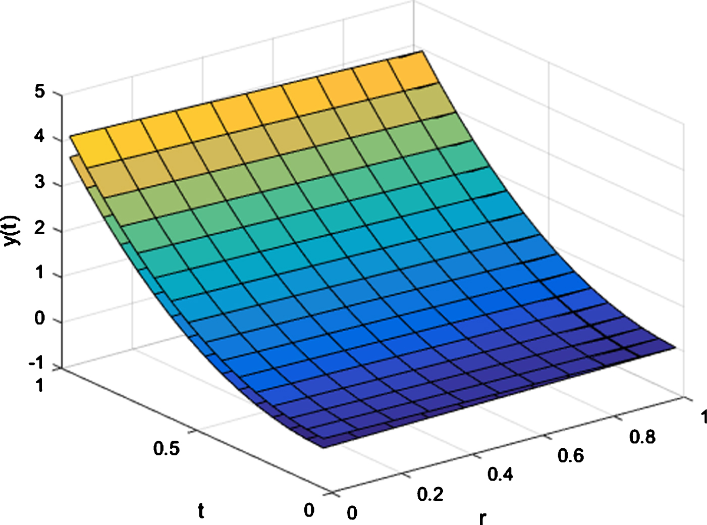
Example 5.2. We consider the following problem: $\begin{array}{l} D_{1, 1}^{(2)} y (t) \oplus & b \otimes (^{c} D_{1, 1}^{1.5} y) (t) \oplus c \otimes y (t) \\ = (1 + t) \otimes (7.9, 8, 8.1), t \in (0, 1], \end{array}$ (47) $y (0) = D_{1}^{(1)} y (0) = (- 0.1, 0, 0.1),$ (48) where b, c ∈ R₊, y ∈ C (J, R_F) and initial values and coefficient of nonhomogeneous term (7.9, 8, 8.1) are triangular fuzzy numbers.

First, we verify the (C1). For any fixed r ∈ [0, 1], we have

$[(- 0.1 0 0.1)]^{r} = [0.1 r - 0.1, 0.1 - 0.1 r],$ $[(7.9, 8, 8.1)]^{r} = [7.9 + 0.1 r, 8.1 - 0.1 r],$ $\begin{matrix} d ([f (t)]^{r}) & = 0.2 (1 + t) (1 - r), d ([y_{0}]^{r} \\ = d ([y_{0}^{'}]^{r} = 0.2 (1 - r), \end{matrix}$ so we should illuminate the integral equation

$U (t) + {bI}_{0 +}^{0.5} U (t) + {cI}_{0 +}^{2} U (t) = 0.2 (1 - r) (1 - c) (1 + t)$ (49)

has nonnegative solution. Denoting operator $LU (t) : = {bI}_{0 +}^{0.5} U (t) + {cI}_{0 +}^{2} U (t)$ , for any b, c, (I + L) is reversible and continuous, and $\begin{matrix} (I + L)^{- 1} & = I - L + L^{2} - L^{3} \dots \\ = (I - L) + L \circ (I - L) \dots . \end{matrix}$

It is sufficient to prove (I - L) (0.2 (1 - r) (1 - c) (1 + t)) ≥0. For the simple consideration, we only consider the case of 1 - c ≥ 0. $\begin{matrix} (I - L) (0.2 (1 - r) (1 - c) (1 + t)) = 0.2 (1 - r) \\ \cdot (1 - c) ((1 + t) - {bI}_{0 +}^{0.5} (1 + t) - {cI}_{0 +}^{2} (1 + t)) \\ = 0.2 (1 - r) (1 - c) ((1 + t) - b \frac{t^{0.5}}{Γ (1.5)} - b \frac{t^{1.5}}{Γ (2.5)} \\ - c \frac{t^{2}}{2} - c \frac{t^{3}}{6}) \\ \geq 0.2 (1 - r) (1 - c) (1 - 1.88063 \cdot b - \frac{2}{3} c) . \end{matrix}$

Therefore, if 1 - c ≥ 0 and $(1 - 1.88063 \cdot b - \frac{2}{3} c) > 0$ , then equation (49) has nonnegative solution.

Next, we verify the (C2).

For r₁, r₂ ∈ [0, 1] , r₁ ≤ r₂, we have f₁ (t, r) = (1 + t) (7.9 + 0.1r). So $\begin{matrix} f_{1} (t, & r_{2}) - f_{1} (t, r_{1}) \\ = (1 + t) (7.9 + 0.1 r_{2}) - (1 + t) (7.9 + 0.1 r_{1}) \\ = (1 + t) 0.1 (r_{2} - r_{1}) \end{matrix}$ and $\begin{matrix} y_{0, 1} (r_{2}) - y_{0, 1} (r_{1}) \\ = 0.1 r_{2} - 0.1 - (0.1 r_{1} - 0.1) = 0.1 (r_{2} - r_{1}), \\ y_{0, 1}^{'} (r_{2}) - y_{0, 1}^{'} (r_{1}) = 0.1 (r_{2} - r_{1}), \end{matrix}$ we get $Δ_{(r_{1}, r_{2})} f_{1} (t) - c (Δ_{(r_{1}, r_{2})} y_{0, 1} + Δ_{(r_{1}, r_{2})} y_{0, 1}^{'} t) = 0.1 (r_{2} - r_{1}) (1 + t) (1 - c)$ .

Therefore, we should prove that $U (t) + {bI}_{0 +}^{0.5} U (t) + {cI}_{0 +}^{2} U (t) = 0.1 (r_{2} - r_{1}) (1 + t) (1 - c)$ has nonnegative solution. From equation (49), it is sufficient if $0.1 (1 - r) (1 - c) (1 - 1.88063 \cdot b - \frac{2}{3} c) \geq 0$ . After all, (C2) is proved.

Finally, we verify the (C3). For r₁, r₂ ∈ [0, 1] , r₁ ≤ r₂, we have f₂ (t, r) = (1 + t) (8.1 - 0.1r). Since f₂ (t, r₂) - f₂ (t, r₁) = -0.1 (1 + t) (r₂ - r₁) and $\begin{matrix} y_{0, 2} (r_{2}) - y_{0, 2} (r_{1}) \\ = 0.1 - 0.1 r_{2} - (0.1 - 0.1 r_{1}) = - 0.1 (r_{2} - r_{1}) \\ y_{0, 2}^{'} (r_{2}) - y_{0, 2}^{'} (r_{1}) = - 0.1 (r_{2} - r_{1}), \end{matrix}$ so we get $Δ_{(r_{1}, r_{2})} f_{2} (t) - c (Δ_{(r_{1}, r_{2})} y_{0, 2} + Δ_{(r_{1}, r_{2})} y_{0, 2}^{'} t) = - 0.1 (r_{2} - r_{1}) (1 + t) (1 - c)$ . After all, we should prove $\begin{matrix} U (t) + {bI}_{0 +}^{0.5} U (t) & + {cI}_{0 +}^{2} U (t) \\ = - 0.1 (r_{2} - r_{1}) (1 + t) (1 - c) \end{matrix}$ has a unique non-positive solution.

For that, we consider the condition for $0.1 (r_{2} - r_{1}) (1 - c) (1 - 1.88063 \cdot b - \frac{2}{3} c) \geq 0$ .

Therefore, in the case of 1 - c ≥ 0, if $(1 - 1.88063 \cdot b - \frac{2}{3} c) > 0$ , then (47), (48) has a unique (1,1)-solution. Numerical results computed by Mathematica 9.0 are shown in Table 2 and 3 in case of b = 0.4, c = 0.3.

Table 2

Numerical results for r = 1 in case of b = 0.4, c = 0.3

t	y₁ (t, 1)	y₂ (t, 1)	$y_{1}^{″} (t, 1)$	$y_{2}^{″} (t, 1)$
0.0625	0.01999	0.01999	7.67726	7.67726
0.1875	0.14062	0.14062	7.93684	7.93684
0.3125	0.38568	0.38568	8.35545	8.35545
0.4375	0.76133	0.76133	8.78868	8.78868
0.5625	1.27428	1.27428	9.2084	9.2084
0.6875	1.93104	1.93104	9.60309	9.60309
0.8125	2.73776	2.73776	9.96684	9.96684
0.9375	3.70013	3.70013	10.2963	10.2963

Table 3

Numerical results for r = 0.5 in case of b = 0.4, c = 0.3

t	y₁ (t, 0.5)	y₂ (t, 0.5)	$y_{1}^{″} (t, 0.5)$	$y_{2}^{″} (t, 0.5)$
0.0625	-0.033212	0.073205	7.64367	7.71085
0.1875	0.080636	0.200616	7.90212	7.97157
0.3125	0.318374	0.452999	8.31889	8.392
0.4375	0.686133	0.836545	8.75023	8.82713
0.5625	1.19058	1.35798	9.16812	9.24869
0.6875	1.83821	2.02386	9.56107	9.6451
0.8125	2.63516	2.84036	9.92323	10.0104
0.9375	3.58706	3.81319	10.2512	10.3413

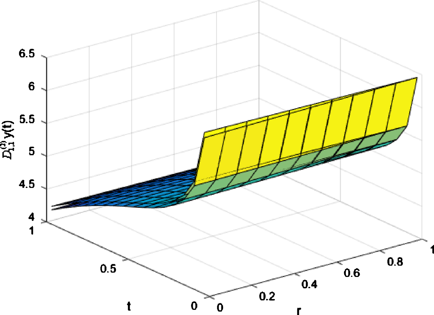
Fig 1 is shown the graph of (1, 1)-solution y (t) and Fig 2 is shown the graph of $D_{1, 1}^{(2)} y (t)$ for Example 5.2 Finally, we consider the problem which has not (1,1)-solution.

Fig. 1

Graph of solution y (t) for Example 5.2.

Fig. 2

Graph of $D_{1, 1}^{(2)} y (t)$ for Example 5.2.

Example 5.3. We find the case that (47), (48) has not (1,1)-solution. It is sufficient to find the case that equation (49) has negative solution. By using multivariate Mittag-Leffelr function, the solution of (49) is expressed as follows: $\begin{matrix} U (t) = 0.2 (1 - r) (1 - c) (1 + t) \\ - 0.2 (1 - r) (1 - c) b \cdot (t^{0.5} E_{(0.5, 2), 1.5} (- {bt}^{0.5}, - {ct}^{2}) \\ + t^{1.5} E_{(0.5, 2), 2.5} (- {bt}^{0.5}, - {ct}^{2})) \\ - 0.2 (1 - r) (1 - c) c \cdot (t^{2} E_{(0.5, 2), 3} (- {bt}^{0.5}, - {ct}^{2}) \\ + t^{3} E_{(0.5, 2), 4} (- {bt}^{0.5}, - {ct}^{2})) . \end{matrix}$

The solution does not exist if there exists t such that $\begin{matrix} T (t, c, b) : = (1 - c) (1 + t) \\ - (1 - c) b \cdot (t^{0.5} E_{(0.5, 2), 1.5} (- {bt}^{0.5}, - {ct}^{2}) \\ + t^{1.5} E_{(0.5, 2), 2.5} (- {bt}^{0.5}, - {ct}^{2})) \\ - (1 - c) c \cdot (t^{2} E_{(0.5, 2), 3} (- {bt}^{0.5}, - {ct}^{2}) \\ + t^{3} E_{(0.5, 2), 4} (- {bt}^{0.5}, - {ct}^{2})) < 0 . \end{matrix}$

Indeed, we see that computing by Mathematica 9.0, T (0.5, 1.5, 1.5) = -0.302214. Table 4 shows that (47), (48) has not (1,1)-solution for b = c = 1.5 by numerical results. In this table, $y_{1}^{″} (t, 0.5) \leq y_{2}^{″} (t, 0.5)$ does not hold for t ∈ J. Fig 3 is shown the graph of y (t) and Fig 4 is shown the graph of $y_{1}^{″} (t, r), y_{2}^{″} (t, r)$ for Example 5.3. In Fig 4, $y_{1}^{″} (t, r) > y_{2}^{″} (t, r)$ , ∀t ∈ J, r ∈ [0, 1]. From Fig 3 and 4, y (t) is not (1,1)-solution of Example 5.3.

Table 4

Numerical results for r = 0.5 in case of b = c = 1.5

t	y₁ (t, 0.5)	y₂ (t, 0.5)	$y_{1}^{″} (t, 0.5)$	$y_{2}^{″} (t, 0.5)$
0.0625	-0.037297	0.068855	6.07804	6.04017
0.1875	0.049291	0.167364	5.25964	5.22687
0.3125	0.219636	0.349109	5.04592	5.01449
0.4375	0.469024	0.609404	4.9093	4.87871
0.5625	0.79515	0.945959	4.78433	4.75452
0.6875	1.196	1.35677	4.64703	4.61808
0.8125	1.6694	1.83969	4.48822	4.46025
0.9375	2.21287	2.39223	4.3048	4.27798

Fig. 3

Graph of solution y (t) for Example 5.3.

Fig. 4

Graph of $D_{1, 1}^{(2)} y (t)$ for Example 5.3.

6 Conclusion

In this paper, we obtain necessary and sufficient condition for the existence of (1,1) and (1,2)-solution to initial value problem for fuzzy Bagley-Torvik equation, and derive the solution representation. Our results show that existence of fuzzy solution depends on the coefficients, nonhomogeneous term and initial value. Our method can be applied to many other types of fuzzy linear multi-term fractional differential equations.

7 Appendix

We can obtain the results of existence and representation for (1,2)-solution in the similar way to section 3 and 4. We omit proof and only show the results in Appendix.

We discuss the following initial value problem for fuzzy Bagley-Torvik equation: $(^{c} D_{1, 2}^{(2)} y) (t) \oplus b \otimes (^{c} D_{1, 2}^{β} y) (t) \oplus c \otimes y (t) = f (t),$ (50) $y (0) = y_{0}, D_{1}^{(1)} y (0) = y_{0}^{'}, t \in (0, 1],$ (51)

where $1 < β < 2, b, c \in R_{+}, y_{0}, y_{0}^{'} \in R_{F}, y, f \in C (J, R_{F}), J = [0, 1]$ .

We get the following cut system by using cut.

${\begin{matrix} y_{2}^{″} (t, r) + b^{c} D_{0 +}^{β} y_{2} (t, r) + {cy}_{1} (t, r) = f_{1} (t, r), \\ y_{1}^{″} (t, r) + b^{c} D_{0 +}^{β} y_{1} (t, r) + {cy}_{2} (t, r) = f_{2} (t, r), \\ y_{1} (t, r) \leq y_{2} (t, r), \\ y_{1}^{'} (t, r) \leq y_{2}^{'} (t, r), \\ ^{c} D_{0 +}^{β} y_{2} (t, r) \leq^{c} D_{0 +}^{β} y_{1} (t, r), \\ y_{2}^{″} (t, r) \leq y_{1}^{″} (t, r), \end{matrix}$ (52)

$\begin{matrix} y_{1} (0, r) = y_{0, 1} (r), y_{1}^{'} (0, r) = y_{0, 1}^{'} (r), \\ y_{2} (0, r) = y_{0, 2} (r), y_{2}^{'} (0, r) = y_{0, 2}^{'} (r) . \end{matrix}$ (53)

Definition A.1. (y₁ (t, r) , y₂ (t, r)) is called solution of problem (52 and (53) if it satisfies (52), (53) and ${y^{″}}_{1} (\cdot, r), {y^{″}}_{2} (\cdot, r) \in C (J)$ .

Theorem A.1. (Necessary condition for the existence of (1,2)-solution)

If y (t) is a (1,2)-solution of (50), (51), then its cut y₁ (t, r) , y₂ (t, r) are solutions of (52), (53) and the followings hold.

(C4) Integral equation with inequality conditions $\begin{matrix} U (t) + {bI}_{0 +}^{2 - β} U (t) - {cI}_{0 +}^{2} U (t) \\ = d ([f (t)]^{r}) - c (d ([y_{0}]^{r}) + d ([y_{0}^{'}]^{r}) t), \end{matrix}$ (54) $I_{0 +}^{2} U (t) \leq d ([y_{0}]^{r}) + d ([y_{0}^{'}]^{r}) t,$ (55) $I_{0 +}^{1} U (t) \leq d ([y_{0}]^{r})$ (56) has a unique nonnegative solution.

(C5) For any r₁, r₂ ∈ [0, 1] (r₁ ≤ r₂), the following system of integral equations with inequality conditions has solution (V (t) , U (t)) satisfying V (t) ≥0, U (t) ≤0:

${\begin{matrix} \begin{matrix} V (t) & + {bI}_{0 +}^{2 - β} V (t) + {cI}_{0 +}^{2} U (t) \\ = Δ_{(r_{1}, r_{2})} f_{1} (t) - c (Δ_{(r_{1}, r_{2})} y_{0, 1} + Δ_{(r_{1}, r_{2})} y_{0, 1}^{'} t), \end{matrix} \\ \begin{matrix} U (t) & + {bI}_{0 +}^{2 - β} U (t) + {cI}_{0 +}^{2} V (t) \\ = Δ_{(r_{1}, r_{2})} f_{2} (t) - c (Δ_{(r_{1}, r_{2})} y_{0, 2} + Δ_{(r_{1}, r_{2})} y_{0, 2}^{'} t), \end{matrix} \end{matrix}$ (57)

${\begin{matrix} Δ_{(r_{1}, r_{2})} y_{0, 1} + Δ_{(r_{1}, r_{2})} y_{0, 1}^{'} t + I_{0 +}^{α} U (t) \geq 0, \\ Δ_{(r_{1}, r_{2})} y_{0, 2} + Δ_{(r_{1}, r_{2})} y_{0, 2}^{'} t + I_{0 +}^{α} V (t) \leq 0, \end{matrix}$ (58) ${\begin{matrix} Δ_{(r_{1}, r_{2})} y_{0, 1}^{'} + I_{0 +}^{1} U (t) \geq 0, \\ Δ_{(r_{1}, r_{2})} y_{0, 2}^{'} + I_{0 +}^{1} V (t) \leq 0, \end{matrix}$ (59)

Theorem A.2. (Sufficient condition for the existence of (1,2)-solution)

If y₁ (t, r) , y₂ (t, r) are the solutions of (52), (53) and (C3), (C4) are satisfied, then fuzzy initial value problem (50), (51) has a unique (1,2)-solution.

Theorem A.3. (Representation of (1,2)-solution)

The representation of (1,2)-solution for fuzzy initial value problem (A.1), (A.2) is as follows: $\begin{matrix} y (t) & = (y_{0} \oplus t \cdot y_{0}^{'} \oplus \sum_{k = 0}^{\infty} c^{2 k} ɛ^{(-)}_{2 - β, 4 k + 2}^{2 k + 1, b} f (t) \\ \oplus y_{0} \sum_{k = 0}^{\infty} c^{2 k + 1} t^{4 k + 2} E^{(+)}_{2 - β, 4 k + 3}^{2 k + 1} ({bt}^{2 - β}) \\ \oplus y_{0}^{'} \sum_{k = 0}^{\infty} c^{2 k} t^{4 k + 3} E^{(-)}_{2 - β, 4 k + 4}^{2 k + 1} ({bt}^{2 - β}) \\ \oplus \sum_{k = 0}^{\infty} c^{2 k + 1} ɛ^{(-)}_{2 - β, 4 k + 2}^{2 (k + 1), b} f (t) \\ \oplus y_{0} \sum_{k = 0}^{\infty} c^{2 (k + 1)} t^{4 k + 4} E^{(+)}_{2 - β, 4 k + 5}^{2 (k + 1)} ({bt}^{2 - β}) \\ \oplus y_{0}^{'} \sum_{k = 0}^{\infty} c^{2 (k + 1)} t^{4 k + 5} E^{(-)}_{2 - β, 4 k + 6}^{2 (k + 1)} ({bt}^{2 - β})) \\ \underset{H}{⊖} (\sum_{k = 0}^{\infty} c^{2 k} ɛ^{(+)}_{2 - β, 4 k + 2}^{2 k + 1, b} f (t) \end{matrix}$ $\begin{matrix} \oplus y_{0} \sum_{k = 0}^{\infty} c^{2 k + 1} t^{4 k + 2} E^{(-)}_{2 - β, 4 k + 3}^{2 k + 1} ({bt}^{2 - β}) \\ \oplus y_{0}^{'} \sum_{k = 0}^{\infty} c^{2 k} t^{4 k + 3} E^{(+)}_{2 - β, 4 k + 4}^{2 k + 1} ({bt}^{2 - β}) \\ \oplus \sum_{k = 0}^{\infty} c^{2 k + 1} ɛ^{(+)}_{2 - β, 4 k + 2}^{2 (k + 1), b} f (t) \\ \oplus y_{0} \sum_{k = 0}^{\infty} c^{2 (k + 1)} t^{4 k + 4} E^{(-)}_{2 - β, 4 k + 5}^{2 (k + 1)} ({bt}^{2 - β}) \\ \oplus y_{0}^{'} \sum_{k = 0}^{\infty} c^{2 (k + 1)} t^{4 k + 5} E^{(+)}_{2 - β, 4 k + 6}^{2 (k + 1)} ({bt}^{2 - β})) \end{matrix}$ (60)

where α, β > 0, $\begin{matrix} ɛ^{(m)}_{β, α}^{ρ λ} f (t) \\ : = \int_{0}^{t} (t - s)^{α - 1} E^{(m)}_{β, α}^{ρ} (- λ (t - s)^{β}) f (s) ds, \end{matrix}$ $E_{β, α}^{ρ} (z) = \sum_{k = 0}^{\infty} \frac{(ρ)_{k}}{k!} \frac{z^{k}}{Γ (α k + β)} .$

References

Agarwal

R.P.

, Lakshmikantham

and Nieto

J.J.

, On the concept of solution for fractional differential equations with uncertainty, Nonlinear Analysis 72 (2010), 2859–2862.

Ahmadian

, Salahshour

, Ali-Akbari

, Ismail

and Baleanu

, A novel approach to approximate fractional derivative with uncertain conditions, Fract Calc Appl Anal 104 (2017), 68–76.

Allahviranloo

, Gouyandeh

and Armand

, Fuzzy fractional differential equations under generalized fuzzy Caputo derivative, J Intell Fuzzy Syst 26 (2014), 1481–1490.

Anastassiou

G.A.

, Fuzzy Mathematics: Approximation Theory, Studies in Fuzziness and Soft Computing 251, Springer-Verlag, Berlin, Heidelberg, (2010).

Arqub

O.A.

and Maayah

, Solutions of Bagley– Torvik and Painleve equations of fractional order using iterative reproducing kernel algorithm with error estimates, Neural Comput Appl 29 (2018), 1465–1479.

Arqub

O.A.

and Smadi

M.A.

, Atangana– Baleanu fractional approach to the solutions of Bagley– Torvik and Painlevé equations in Hilbert space, Chaos Solitons Fractals 117 (2018), 161–167.

Arshad

, On existence and uniqueness of solutions of fuzzy fractional differential equations, Iran J Fuzzy Syst 10 (2013), 137–151.

Bagley

R.L.

and Torvik

P.J.

, On the appearance of the fractional derivative in the behavior of real materials, ASME Trans J Appl Mech 51 (1984), 294–298.

Bede

and Stefanini

, Generalized differentiability of fuzzyvalued functions, Fuzzy Sets Syst 230 (2013), 119–141.

10.

Chakraverty

, Tapaswini

and Behera

, Fuzzy Arbitrary Order System: Fuzzy Fractional Differential Equations and Applications, John Wiley & Sons, Inc., Hoboken, New Jersey, (2016).

11.

Cenesiz

, Keskin

and Kurnaz

, The solution of the Bagley– Torvik equation with the generalized Taylor collocation method, J Franklin I 347 (2010), 452–466.

12.

Hoa

N.V.

, On the initial value problem for fuzzy differential equations of non-integer order α ∈ (1, 2), Soft Comput https://doi.org/10.1007/s00500-019-04619-7.

13.

Hoa

N.V.

, Fuzzy fractional functional integral and differential equations, Fuzzy Sets Syst 280 (2015), 58–90.

14.

Hoa

N.V.

, Lupulescu

and O’Regan

, A note on initial value problems for fractional fuzzy differential equations, Fuzzy Sets Syst 347 (2018), 54–69.

15.

Hoa

N.V.

, Tri

P.V.

, Dao

T.T.

and Zelinka

, Some global existence results and stability theorem for fuzzy functional differential equations, J Intell Fuzzy Syst 28 (2015), 393–409.

16.

Karaaslana

M.F.

, Celiker

and Kurulay

, Approximate solution of the Bagley– Torvik equation by hybridizable discontinuous Galerkin methods, Appl Math Comput 285 (2016), 51–58.

17.

Mashayekhi

and Razzaghi

, Numerical solution of the fractional Bagley-Torvik equation by using hybrid functions approximation, Math Method Appl Sci 39 (2016), 353–365.

18.

Moghaddam

B.P.

, Machado

J.A.T.

and Behforooz

, An integro quadratic spline approach for a class of variable-order fractional initial value problems, Chaos Solitons Fractals 102 (2017), 354–360.

19.

Mohammadi

and Mohyud-Din

S.T.

, A fractional-order Legendre collocation method for solving the Bagley-Torvik equations, Adv Differ Equ 2016 (2016), 269.

20.

Prakash

, Nieto

J.J.

, Senthilvelavan

and Sudha Priya

, Fuzzy fractional initial value problem, J Intell Fuzzy Syst 28 (2015), 2691–2704.

21.

Raja

M.A.Z.

, Samar

, Manzar

M.A.

and Shah

S.M.

Design of unsupervised fractional neural network model optimized with interior point algorithm for solving Bagley-Torvik equation, Math Comput Simulat https://dx-doi-org.web.bisu.edu.cn/10.1016/j.matcom.2016.08.002.

22.

Ray

S.S.

, On Haar wavelet operational matrix of general order and its application for the numerical solution of fractional Bagley Torvik equation, Appl Math Comput 218 (2012), 5239–5248.

23.

Ray

S.S.

and Bera

R.K.

, Analytical solution of the Bagley Torvik equation by Adomian decomposition method, Appl Math Comput 168 (2005), 398–410.

24.

Salahshour

, Allahviranloo

, Abbasbandy

and Baleanu

, Existence and uniqueness results for fractional differential equations with uncertainty, Adv Differ Equ 2012 (2012), 112.

25.

Stanek

, Two-point boundary value problems for the generalized Bagley– Torvik fractional di?erential equation, Cent Eur J Math 11 (2013), 574–593.

26.

Stanek

, The Neumann problem for the generalized Bagley-Torvik fractional differential equation, Fract Calc Appl Anal 19 (2016), 907–920.

27.

Wang

Z.H.

and Wang

, General solution of the Bagley– Torvik equation with fractional-order derivative, Commun Nonlinear Sci Numer Simulat 15 (2010), 1279–1285.

28.

Youssri

Y.H.

, A new operational matrix of Caputo fractional derivatives of Fermat polynomials: an application for solving the Bagley-Torvik equation, Adv Differ Equ 2017 (2017), 73.

29.

Zahoor

R.M.A.

, Khan

J.A.

and Qureshi

I.M.

, Solution of Fractional Order System of Bagley-Torvik Equation Using Evolutionary Computational Intelligence, Math Probl Eng 18. doi:10.1155/2011/675075

30.

Zahra

W.K.

and Daele

M.V.

, Discrete spline methods for solving two point fractional Bagley– Torvik equation, Appl Math Comput 296 (2017), 42–56.

31.

Sin

, Chen

, Choi

and Ri

, Fractional Jacobi operational matrix for solving fuzzy fractional diferential equation, J Intell Fuzzy Syst 33 (2017), 1041–1052.

32.

Sin

, Chen

, Wu

, R

and Choi

, Application of a spectral method to fractional diferential equations under un certainty, J Intell Fuzzy Syst 35 (2018), 4821–4835.

33.

Choi

, Kwon

, Sin

, Pak

and So

, Constructive Existence of (1,1)-Solutions to Two-Point Value Problems for Fuzzy Linear Multiterm Fractional Differential Equations, Abstr Appl Anal (2019), Article ID 5129013.

34.

Alaroud

, Al-Smadi

, Ahmad

R.R.

and Din

U.K.S.

, An Analytical Numerical Method for Solving Fuzzy Fractional Volterra Integro-Differential Equations, Symmetry 11 (2019), 205.

35.

Alarouda

, Ahmada

R.R.

and Din

U.K.S.

, An Efficient Analytical Numerical Technique for Handling Model of Fuzzy Differential Equations of Fractional-Order, Filomat 33(2) (2019), 617–632.

36.

Luchko

and Gorenflo

, An Operational Method for Solving Fractional Differential Equations with the Caputo Derivatives, Acta Mathematica Vietnamica 24(2) (1999), 207–233.

37.

Chehlabi

and Allahviranloo

, Concreted solutions to fuzzy linear fractional differential equations, Appl Soft Comput 44 (2016), 108–116.

38.

Allahviranloo

, Abbasbandy

and Rouhparvar

, The exact solutions of fuzzy wave-like equations with variable coefficients by a variational iteration method, Appl Soft Comput 11 (2011), 2186–2192.

39.

Haydar

A.K.

and Hassan

R.H.

, Generalization of Fuzzy Laplace Transforms of Fuzzy Fractional Derivatives about the General Fractional Order n – 1 β < n, Math Probl Eng Article ID 6380978, (2016), 13.