Multi-armed bandits for bid shading in first-price real-time bidding auctions

Working out the best amount to bid in first-price ad auctions can save much money for the ad buyer. When tens or hundreds of millions of auctions are processed daily, saving just a little bit of money per auction builds quickly. However, when the number of other participants in the auctions is unknown, it may be hard to figure out the right amount to bid. The number of other participants varies, and the participants will have their bidding strategies. These factors result in a complex environment where there are many unknown factors.

This research aims to investigate how to optimize the bid size in first-price auctions. First, we will use data from second-price auctions to simulate first-price auction data. Then, the study will focus on finding out the least amount to win the auction in a specific situation. The amount may change depending on different factors like weekdays or times of the day. The goal is to find a way to estimate the winning price as close as possible by testing and comparing different multi-armed bandit algorithms. We used these methods because they are easy to tune, robust, lightweight, and easy to implement [7, 8]. Moreover, we focused on a subset of their most straightforward and well-known versions because these are more attractive for industrial purposes. Upon comparison, the best methods will be tested in a production environment, and then we analyze their performance and discuss their limitations.

1.2 Data and methods

This paper will use data from real OpenRTB auctions happening through a real Demand Side Platform (DSP): ReadPeak 2 /. ReadPeak is a platform that enables advertisers to promote their content online. ReadPeak makes it easy for advertisers to buy inventory from a publisher that they choose. The auction data will contain the auction timestamp and information on the bid request, like the requesting publisher and the ad placement on the page. The data will also contain the bid sizes that were bid and the information whether the bid won the auction or not. The data will only contain the winning bid amounts for the bids won by a bid from the ReadPeak’s DSP. The other bid sizes will be unknown. This research will evaluate how multi-armed bandit strategies will work in optimizing the bid size in ReadPeak’s first-price real-time bidding environments. The amount to bid will be given a range, and the range will be divided into slots where each slot acts as a bandit’s arm. Different bandit algorithms will be evaluated against each other to find the best performing one. The bandit algorithms will be compared with the baseline of always bidding the impression’s maximum value (naïve approach). The best three algorithms will be evaluated in the production environment. This study will research only multi-armed bandit algorithms and determine whether they are suitable and efficient in solving this problem.

1.3 Related work

In recent years, bid optimization in real-time bidding has been studied extensively. In [9], the authors consider the problem of acquiring a given number of impressions with a given budget. They consider both cases where all of the winning bids are known, and only bids made by the bidder are known. In their approach, the algorithm learns the other bidders’ distribution in the exploration phase and then bids against that. They consider the other bidders’ bid distribution of remaining the same, which may not be accurate in modern header bidding environments.

Another approach to device a bidding strategy is to try to forecast the advertising campaigns’ bid distribution, as is done by the authors in [10]. They use historical bidding data to build a gradient boosting decision tree to forecast the bid distribution. Then, they aim to estimate how many impressions an advertiser will win by bidding a certain amount. This approach may work to some extent; however, it does not consider the non-stationary nature of the bid landscape. Most of the previous work on bid optimization has focused on second-price auctions, as is the case in the above studies. The authors in [11] present a bidding strategy to optimize the bidding price and compare the outcome of three different bidding price strategies.

A lot of the bid optimization research has focused on search-based auctions. The authors in [12] consider the bid optimization problem faced by an advertiser where they want to get as much value (clicks) for the budget. They cast the problem as a Markov Decision Process [13] with censored observations and propose a learning method based on the Kaplan-Meier method [14]. Although they also consider second-price auctions, this is the same goal that we want to achieve in our research.

Repeated auction theory has been researched from the sellers’ perspectives also. The researchers in [12] propose an algorithm for the seller to optimize the floor price against strategic (non-truthful) bidders. The authors view the problem as a bandit problem. However, they note that a traditional bandit algorithm like Upper Confidence Bound (UCB) [15] or Exponential-weight algorithm for Exploration and Exploitation (EXP3) [16] may not perform well as the buyer may strategically adjust the bidding once the seller’s algorithm reaches a price it considers optimal. The authors in [17] propose models to combat these situations where the reward structure may change. They propose a model for stochastic and adversarial cases. For the stochastic model, the authors proposed an UCB-type algorithm. The adversarial bandit problems are tricky for algorithms like UCB, as they will not react very quickly to the changing rewards. The authors propose an algorithm based on EXP3 as the standard EXP3 algorithm is designed for a finite number of actions. In their auction setup, the number of actions is unbounded.

In [11], the authors suggested that the best bidding strategy was linearly related to the predicted CTR of the ad. The authors in [18] were among the first to discover the non-linear relationship between the optimal bid and the impression evaluation. Their research suggests that one should try to bid more on low-price impressions than focus on high-value impressions. The authors in [19] also show that the linear method performs well in second-price auctions.

The issue with censored data in real-time bidding environments is approached in [20] and [21]. In [20], the authors show that training regression models based on only the winning price would be overfitting to the winning bids, which are generally higher than the losing bids. In [21], the authors are also able to tackle the issue with bias in learning using censored data.

Low regret learning algorithms for figuring out the right amount to bid are presented in [22]. These consider a setting where a seller (publisher) chooses the buyer (ad exchange) in advance based on the historical bidding data. The authors in [22] compare their algorithms with the EXP3 algorithm. They do not expect the EXP3 algorithm to perform well in their setting, as they expect the publisher to use a no-regret algorithm.

The authors in [23] proposed the first deep reinforcement learning agent for optimizing the bidding. They use the agent on JD.com. At first, JD.com used a bidding approach based on eCPM where they predict the CTR. At last, they developed an agent based on a variant of Deep Q Network (DQN) [24]. They encode each auction request data (user data, product IDs, and ads) into plain text. They one-hot encode the text and feed it to a deep convolutional neural network. The agent’s state is defined as the data they have about the user, product IDs, and ads.

The state-of-the-art research in bid optimization is focusing nowadays on reinforcement learning to optimize bidding behavior. In [25], the authors build a Markov Decision Process framework to figure out the best bidding strategy. As in [23], they divide the flow of auctions into episodes.

In [26] the authors implement a multi-agent bidding solution where the agents cooperate to find the optimal bidding strategies that will benefit all of the bidders. The study most close to our research is presented in [27]. The authors aim to maximize an SSP’s revenue in competing with other bidders in first-price header bidding auctions. The method uses a version of Thompson Sampling combined with particle filtering. Our study compares their bidding strategy with other bandit strategies designed for non-stationary environments, e.g., policies that forget the past observations at a specific rate.

2.1 Strategy

The problem of figuring out the right amount to bid in consecutive real-time bidding auctions can be considered an exploration-exploitation dilemma. We might know an amount that wins the auction, but do we get the best reward (the lowest price) by bidding that amount. We can describe the bidding problem as a multi-armed problem by dividing the bid amounts into the arms and finding out the best way to pull the arms to maximize the total reward or minimize the total amount paid to win the auctions.

We tested the algorithms using data collected from the ReadPeak advertising platform. The data is gathered from the internal auctions happening within the ReadPeak platform and the data received from the external ad exchange. The platform collects data of every auction, bid response, and impression notification.

The data is sent to a data lake from which the data can be fetched for analysis. We first run an internal auction to determine the ad sent to the external ad exchange. Each advertiser has set a bid they are willing to pay for a click. The ad’s bid and CTR are used to calculate the actual bid amount used in the auction. In these auctions, all the participants and their bid amounts are known. However, the other participants in the external ad exchange’s auctions are unknown, and the winning price is known only if our ad wins the impression.

The algorithms will use the bid amount of the winner of the internal auction and the winning price of the exchanges auction. The winning price of the exchange’s auction is the minimum that needs to be bid to win the auction. Our algorithm should try to set the bid amount as close to this as possible, but not lower. The maximum amount the algorithm may bid is the bid amount of the internal auction winner. More importantly, the regret (the inverse of the reward) for each algorithm is calculated as the difference between the winning price and the bid amount.

We will run experiments on two separate datasets. The two datasets contain data from two different publishers located in the UK. For the first dataset, the bidding is done through the Taboola platform 3 , and the auctions are second-price auctions. The first dataset contains data from December 16th to December 18th, 2018. The dataset contains 708 265 auctions. The second dataset contains data for bids done through the AppNexus marketplace 4 . The auctions are second-price auctions, and the dataset includes 348 875 auctions from January 20th to January 26th, 2019. In Fig.2, both datasets are represented, there the winning price is shown in red and the maximum bid is shown in blue.

OPEN IN VIEWER

Fig. 2

The winning prices and the maximum bids for both, top: dataset 1 and bottom: dataset 2.

OPEN IN VIEWER

Fig. 3

General scheme of a bandit algorithm: 1. The maximum amount the advertiser is willing to pay for the impression is fed to the bandit algorithm, 2. The bandit algorithm selects the arm based on the arm rewards. Each arm represents a bid amount in the range [0.05, 0.10,..., 99.95, 100] cents. The selected bid will not exceed the maximum amount the advertiser is willing to pay for the impression, 3. The bid is sent to the auction, 4. Bid wins or loses the auction, and 5. Feedback from the auction is fed to the bandit algorithm, which updates the rewards for the arms.

In dataset 1, the winning and maximum bid sizes are relatively small compared to dataset 2. In dataset 2, there are more considerable differences also with the maximum bid and the winning price than in dataset 1. If the maximum amount that can be bid is larger than the winning price, the algorithm has more room to experiment with different bid sizes.

For each algorithm, we will calculate the cumulative average cost per impression and the win percentage. The lower the cost per impression, and the higher the winning percentage, the better. The auction environment will be simulated by using the collected auction data. In each round, we will check how the bid, chosen by the algorithm, performs against the winning price and keep track of the cumulative average cost per impression and the win percent. The bid chosen by the algorithm will be capped at the bid amount of the internal auction winner. In Fig. 3, a scheme of a bandit algorithm is depicted as well as a detailed description of each step. The auctions will be run in order using the timestamps of the data. We will also look at the run time of the algorithms. A rough requirement for commercial platforms is that the algorithm should run in less than a millisecond. This is because an average time of 200 milliseconds is necessary to provide the bid response to the bid request. This time includes the network latency, the ad selection process from the internal auction, and any other internal calculations. Lastly, we will select the three best-performing algorithms to be tested in the production environment. The algorithms will be tested by running them simultaneously alongside a no algorithm baseline. The no algorithm baseline always bids the eCPM amount of the ad that won the internal auction.

3.1 The ε-greedy algorithm

The ε-greedy algorithm works by exploiting the best arm most of the time and exploring other arms the rest of the time. The epsilon (ε) parameter defines how much to explore versus exploit. The action (A) calculated by ε-greedy algorithm can be described as presented in Eq. (1).

A = { arg max a Q ( a ) with probability 1 - ε a random action with probability ε(1)

Q (a) is the estimated value of action a at time step [15]. best arm is determined by the average reward gained by the arm so far. The reward for the arm on each round is normalized and is calculated by formula in Eq. (2).

arm reward = { 0 if the auction is lost ( max bid - bid ) max bid if wins(2)

Table 1 shows how different epsilon parameter values affect the auctions’ win rate run on datasets 1 and 2. The cumulative average costs per impression are presented in Fig. 4. The averages for dataset 2 are a bit more spread out than for dataset 1. For dataset 1, the average costs per impression are very close to each other. However, the win percentages differ some. With dataset 2, the difference in the impression cost is more considerable. The algorithm with the epsilon parameter 0.01 (explores 1%of the time) seems to perform the best when considering the winning percentages and the cumulative average cost per impression.

OPEN IN VIEWER

Fig. 4

The cumulative average cost per impression for the ε-Greedy algorithms with different values of ε for both, top: dataset 1 and bottom: dataset 2.

The sliding window Upper Confidence Bound (UCB) algorithm (SW-UCB) contains two parameters, the window size, and the exploration multiplier. The exploration multiplier defines how large the exploration term is relative to the average reward. This algorithm works just like the regular UCB algorithm except that it considers only the last N rewards played by the algorithm. Upon selecting the arm randomly, for each round, we select the arm that has the maximum performance calculated by the formula of Eq. (3).

C w + ( c * ln ( min ( n , w ) ) n w ) ,(3)

OPEN IN VIEWER

Fig. 5

The cumulative average cost per impression for the SW-UCB algorithms with different window sizes for both, top: dataset 1 and bottom: dataset 2.

C _w is the average reward in the window, n is the number of rounds played, w is the window size, n _w  > 0 is the number of rounds played by the arm within the window, and c > 0 controls the degree of exploration. The average reward is calculated by taking the average of the rewards in the window. Testing showed that a value of c of 0.2 was the best, and that value is used in the experiments. Table 1 shows the win rates for the tested window sizes on the two datasets.

Figure 2. shows the cumulative average costs per impression for the SW-UCB algorithms with different window sizes. Here the differences are more massive than with dataset 1. On dataset 1, the differences with average costs per impression are relatively small. Interestingly, the smaller window sizes look to have better win rates, although the differences are minor. On dataset 2, the spread with the average cost per impression is more extensive than for dataset 1. Window size 500 seems to generate the right mix of win percent and costs per impression.

The Exponentially Decaying UCB algorithm (ED-UCB) contains a parameter that indicates how fast the old values decay. The smaller the value, the faster the old values are forgotten. The update of the average rewards are estimated with the formula C = (1 - dr) x + dC, where 0 < dr < 1 is the rate of decay and x is the reward received. After selecting an arm to play randomly, on each round, the selected arm with the maximum performance is found using Eq. (4).

C ed + ( c * ln n n t ) ,(4)

C _ed is the exponentially decaying weighted average, n is the number of rounds played, n _t  > 0 is the number of rounds played by the arm, and c > 0 is the parameter that controls the exploration. Table 1 shows the win rates for the ED-UCB algorithm with different decay rates on datasets 1 and 2. Figure. 6 shows the cumulative average cost per impression for the different ED-UCB algorithm variations on dataset 1 and dataset 2.

OPEN IN VIEWER

Fig. 6

The cumulative average cost per impression for the ED-UCB algorithms with different decay rates for both, top: dataset 1 and bottom: dataset 2.

On dataset 1, the differences with the average impression costs are relatively small, although the algorithm with a decay rate of 0.99 looks to stand out. On dataset 2, the differences in the impression costs are more significant than on dataset 1. The algorithm using the decay rate of 0.99 looks to be a clear winner on both datasets.

The Exponentially Decaying Sliding Window UCB (EDSW-UCB) algorithm is a novel proposed method that contains two parameters that can be used to control how fast the algorithm adapts to changes in the environment [38]. The parameters are the window size and the decay rate. This method works as follows, first upon selecting an arm randomly, then on each round, we select the arm with the maximum performance calculated using Eq. (5).

C d + ( c * ln n n t ) ,(5)

C _d is the exponential decaying average reward in the window, n is the number of rounds played, w is the window size, n _w  > 0 is the number of rounds played by the arm, and c > 0 is the exploration parameter. C _d is calculated by iterating over the rewards in the window starting from the oldest values as C_d+1 = C_d+1 * dr + C _d  * (1 - dr), where dr is the decay rate. Preliminary tests indicate that a decay rate of 0.99 seems to perform the best. Table 1 shows how different window sizes affect the win rate on datasets 1 and 2 with the EDSW-UCB algorithm using a decay rate of 0.99. Figure 7 contains the EDSW-UCB algorithms average impression costs on dataset 1 and dataset 2.

OPEN IN VIEWER

Fig. 7

The cumulative average cost per impression for the EDSW-UCB algorithms with decay rate of 0.99 and different window sizes for both, top: dataset 1 and bottom: dataset 2.

The differences between the algorithms are very small on both datasets. The window size of 2500 performs worst on dataset 2. The window size of 12000 shows the best performance.

The Thompson Sampling algorithm differs from the previously analyzed algorithms because it is possible to target a specific win rate with this method. Each arm uses a beta distribution to model a specific win rate. This means that it is possible to choose the win rate for each bid dynamically. The algorithm works as follows, first, each arm is set as a uniform prior beta distribution Beta(α, β) with α, β = 1. Then a random value is drawn from each distribution, then the arm with the value closest to the targeted win rate is selected, and finally, the distribution is updated.

Table 2 shows how modifying the targeted win rate parameter affects the actual win rate on datasets 1 and 2. The algorithm can follow the targeted win rate quite well. With dataset 2, the actual win rate seems to follow the target win rate even better than dataset 1. Figure 8. shows the TS algorithms’ average impression costs on dataset 1 and dataset 2.

OPEN IN VIEWER

Fig. 8

Thompson Sampling cumulative average cost per impression for the different target win rates for both, top: dataset 1 and bottom: dataset 2.

Most of the previous algorithms’ win rates are close to 90 %. We choose 90 %as the target win rate for the Dynamic Thompson Sampling (D-TS) algorithms. The target win rate can be dynamically changed in practice depending on the state in the bidding environment. The Dynamic Thompson Sampling algorithm uses a threshold parameter c to state how fast the alpha and beta values decay. This value controls how the values are updated on each iteration, therefore α n = ( α n - 1 + r ) * c c + 1 and β n = ( β n - 1 + 1 - r ) * c c + 1 , where the reward r is 1 if the arm won and 0 if it lost. Using this formula it is ensured that the algorithm explores and adapts to changes in the environment.

Table 2 shows how the threshold parameter affects the win rate on the two datasets. Figure 9 shows the D-TS algorithms’ average impression costs on dataset 1 and dataset 2.

OPEN IN VIEWER

Fig. 9

The cumulative average cost per impression for the D-TS algorithms with target win rate of 0.9 and different threshold values for both, top: dataset 1 and bottom: dataset 2.

The differences between the algorithms with different thresholds are relatively small on dataset 1. On dataset 2, the differences can be seen more clearly, although the best performing algorithms are very close. Overall, the best performing algorithm looks to be the one with a threshold value of 5000. However, a closer analysis should be done in the production environment with the different threshold values and target win rates.

To see how the algorithms perform compared to each other, we simultaneously ran the best versions of each algorithm. Table 3 shows the win rates for each algorithm on datasets 1 and 2.

Figure 10 shows how the algorithms perform compared to each other on dataset 1 and dataset 2 regarding the cumulative average impression costs.

OPEN IN VIEWER

Fig. 10

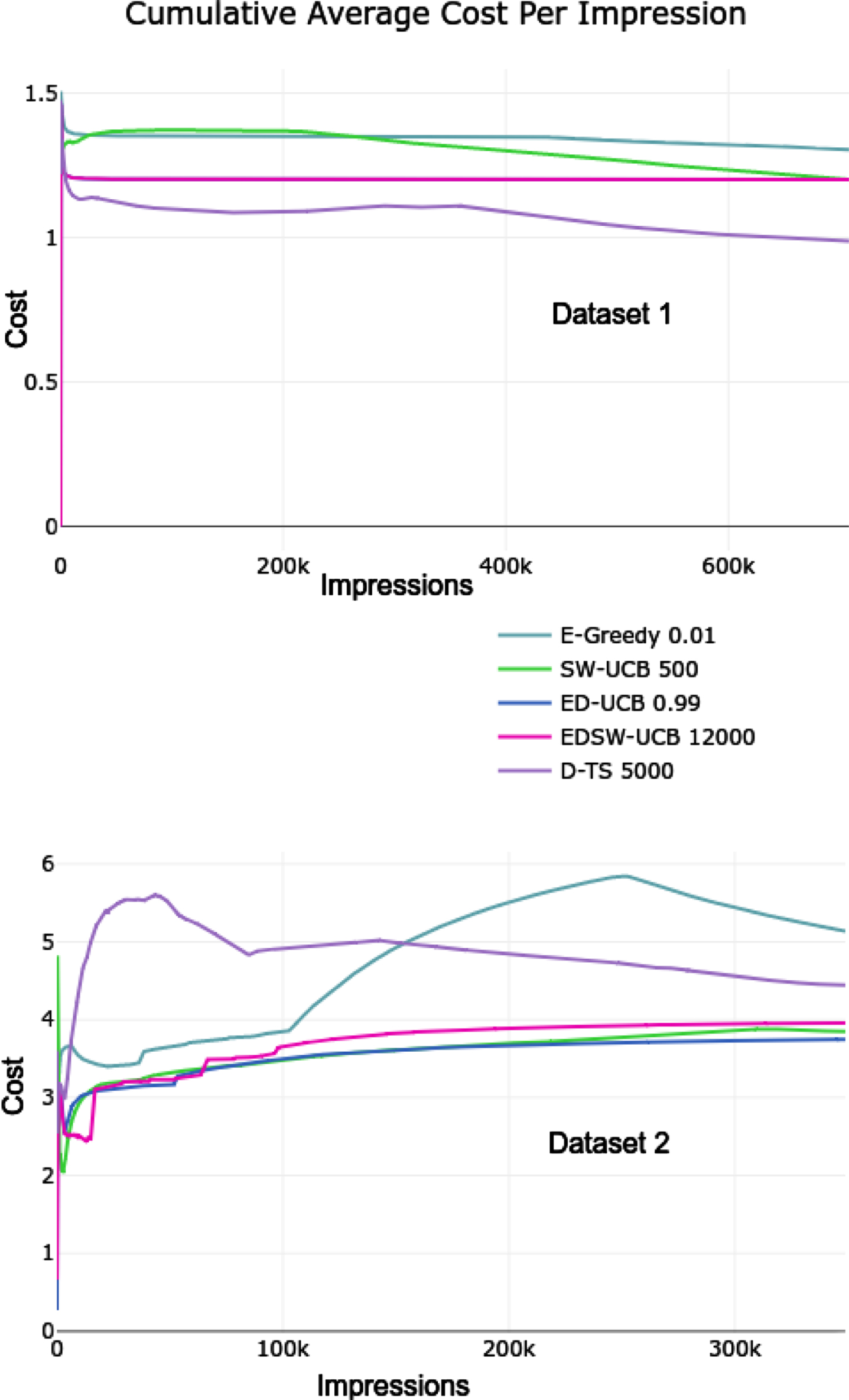
The cumulative average cost per impression for the best versions of each algorithm for both top: dataset 1 and bottom: dataset 2.

The D-TS performs the best on dataset 1, and the ED-UCB performs the best on dataset 2. On dataset 1, regarding the average cost per impression, the D-TS is a clear winner. However, the win rate is a bit lower than for the other algorithms. The ED-UCB performs the second-best on dataset 1. On dataset 2, the D-TS algorithm explores unplayed arms much more than the other algorithms. This explains why the D-TS bids higher than the other algorithms at the beginning of dataset 2, where the maximum bid is much higher than the winning price. The ε-Greedy, ED-UCB, and D-TS algorithms have much better win rates than the SW-UCB and EDWS-UCB algorithms on dataset 2.

The algorithms selected to be tested in production are the ε-Greedy (ε=0.01), ED-UCB (decay rate=0.99), and the D-TS (target win rate=0.9, threshold=5000). We pick the ε-greedy algorithm because it consistently produces high win rates. It is also the most straightforward algorithm, making it interesting to see how it performs in the production environment. The ED-UCB algorithm performs well overall. It is also efficient and straightforward to implement. The D-TS algorithm looks to produce good results regarding the win rate and the average cost per impression. The D-TS algorithm makes it easy to change the target win rate depending on the situation dynamically. This is the perfect situation within the bidding process.

The run time of each algorithm was recorded within the simulated auctions. The algorithms were run in a NodeJS environment on an Intel Core i5-6600K CPU @ 3.50 GHz with 16 GB of RAM. The run times are listed in Table 3. The run time is the average of all the rounds and the different versions of the algorithms. For some of the algorithms, the run time differs depending on the parameters. For instance, for the SW-UCB and EDSW-UCB algorithms, the run times went up when the window size got more prominent. This makes sense as it is required to do more calculations; the larger the window size is.

The EDSW-UCB algorithm is the slowest of the algorithms. All of the algorithms run fast enough for our use case as the limit is one millisecond. Suppose the difference between the performance of the algorithms is close. In that case, it may make sense to select a faster algorithm as the computation needed is larger, the slower the algorithm, and this situation is economically more costly.

3.9 Production results

We have tested the three chosen algorithms D-TS (target win rate=0.9, threshold=5000), ED-UCB (decay rate=0.99), and ε-Greedy (ε=0.01) against a no algorithm baseline in production. The no algorithm baseline always bids the eCPM amount of the ad. Within one publisher, there may be multiple ad placements. We run the algorithms separately for each placement. The algorithm data is saved periodically.

We ran experiments on the algorithms on ad placement on a Norwegian publisher’s site from April 9th of 2019 to April 23rd of 2019 (2 weeks approximately). We ran 4434483 bids, which resulted in 540093 impressions. The placement uses first-price auctions, and the bidding is done through the AppNexus platform.

Note here that all of the three algorithms tested in production suffered from a cold start problem. The cold start problem is caused by the fact that there is no data about the environment when the algorithms are initialized. This means that every time the algorithms are initialized, each arm is on the same level, and the algorithms will need to learn again which arms are best for the specific environment. New instances of the algorithms are spawned several times a day; thus, this has undoubtedly affected the production results. This is a well-known problem, and some studies have been done in the last years to fix it within the multi-armed bandits’ problems [39, 40].

Table 4 shows the win rates for the algorithms running in the placement. It should be noted that the eCPM bid for the ads is relatively low on placement, which means that the win rates will be low compared to the offline results. Further research is required on analyzing how changing the target win rate on the D-TS algorithm will affect the win rate in this case.

Figure 11 shows the average bids per day for the algorithms bidding in the ad placement. There is an apparent rise in the baseline bid amount on the 16th. This may happen due to a new campaign starting or an old campaign stopping from running in the placement. Also, a running campaign may value the impressions differently as the campaign progresses. Figure 11 shows the average impression cost by day for the placement. Table 4 shows the total average impression costs for the algorithms running in the placement.

OPEN IN VIEWER

Fig. 11

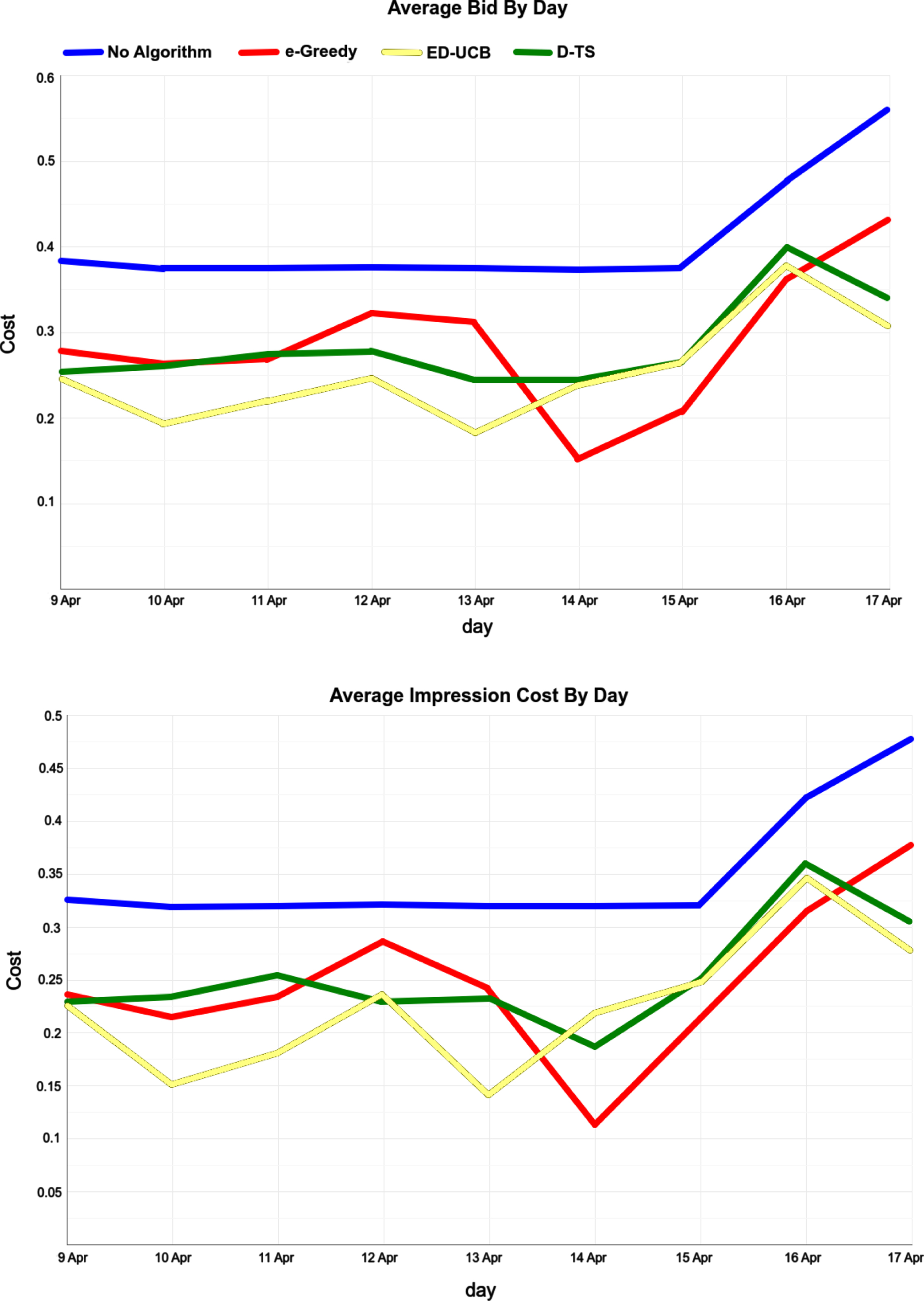
top: average bids and bottom: average impression cost by day for the algorithms done through the ReadPeak platform for a placement on a Norwegian publisher.

The win percentage for the algorithms decreased 7.4%to 8.3%from the baseline. However, the average impression cost decreased as much as 25.9%to 31.9%. This indicates that the benefit of using the bidding algorithms in first-price auctions is substantial. It is clear from the results in Figure 11 that the bid algorithms do an excellent job of lowering the bidding costs. The algorithms’ performance shows some fluctuation as a function of the days compared to each other. Still, the performance is better than the baseline method.