
Abstract
Deep learning (DL) algorithms, especially the convolutional neural network (CNN), have been proven as a newly developed tool in machinery intelligent diagnosis. However, the current CNN-based fault diagnosis studies usually consider features or images extracted from a single domain as model input. This single domain information may not reflect fault patterns comprehensively, leading to low modeling accuracy and inaccurate diagnostic results. To overcome this limitation, this paper proposes a new CNN-based fault diagnosis approach using image representation considering multi-domain features of vibration signals. First, multi-domain features of vibration signals are extracted. These extracted features are then used to construct a n × n matrix, and subsequently to form images by RGB color transformations. This image transformation technique allows for capturing complementary and rich diagnostic information from multiple domains. At last, these images associated with different mechanical defects are fed into a CNN model that is improved based on the classic LeNet-5 CNN architecture for fault diagnosis and identification. Comparative experiments with the traditional feature extraction methods as well as state-of-the-art CNN-based methods are also investigated. Experimental studies on rolling bearings validate the effectiveness and superiorities of the proposed approach.
Keywords
Introduction
Rolling element bearings that support and guide rotating or oscillating machine elements (e.g. shafts, axles or wheels) and transfer loads between machine components, have been playing an increasing part in modern industries. In practice, faulty bearings contribute to most of the failures in rotating machinery, and therefore the identification of bearing faults is of significance [1–3].
The typical bearing fault diagnosis framework involves data acquisition, feature extraction and selection, and pattern recognition [4]. Numerous efforts have been made to develop feature extraction techniques based on vibration signals from the time, frequency and time-frequency domains [5–8]. Afterward, feature selection becomes an essential step in order to improve relevancy and reduce redundancy among a variety of extracted features. At last, the selected features are fed into a shallow model with at most three layers (e.g. input, output, and one hidden layer) to carry out classification or prediction tasks. In general, the shallow learning (also known as traditional machine learning (ML)) is carried out with a separate step. Each stage consumes massive computing resources and highly depends on manual intervention. Besides, The errors in each process will inevitably propagate to the next stage and lead to greater inaccuracy at last.
The DL is part of a broader family of ML based on artificial neural networks [9–11], and it has been widely used in various areas in modern lives, such as visual processing, autopilot, bioinformatics and industrial cyber-physical systems [12, 13]. Both DL and shallow learning belong to data-driven artificial intelligence techniques establishing the complex model relationship between input and output. However, the DL combines feature learning and model building in an end-to-end step by automatically selecting kernel functions and optimizing related parameters [14]. Among various DL techniques, the CNN has recently drawn increasing attention due to its merits, e.g. local connectivity and parameter sharing [15–17].
Since 2015, the CNN has been actively utilized in the area of intelligent fault diagnosis. Chen et al. [18] directly used traditional features as a vector input to a CNN model consisting of one convolutional layer and one pooling layer for gearbox fault identification. Zeng et al. [19] investigated hybrid fault classification by inputting time-frequency images generated by S-transform into a seven-layer CNN. The other two DL algorithms including deep belief network (DBN) and stacked auto-encoder (SAE) were used for comparison. Wang et al. [20] presented a wavelet scalogram as CNN inputs to carry out different status recognition of the rotor experiment, and the results yielding 96% classification accuracy verified its validity. Verstraete et al. [21] proposed an improved CNN of 11 layers using wavelet scalogram images, STFT spectrogram and HHT images for fault diagnosis. Jiang et al. [22] proposed a novel multi-scale CNN model to identify different health conditions of wind turbine gearbox automatically. Eren et al. [23] presented a compact adaptive 1D CNN model, and its performance on a bearing fault diagnosis system was extensively studied. Chen et al. [24] proposed a hybrid of cyclic spectral coherence and CNN to conduct rolling bearing classification. The new model was validated by the public Case Western Reserve University bearing fault.
In recent five years, especially in the last two years, much attention has been drawn to the CNN-based fault diagnosis. However, the current CNN-based diagnostic models are usually limited by their input data type or incomplete information extracted only from a single domain. For example, some studies consider the feature values extracted from vibration signals as the direct input of CNN model. The value input to CNN is not helpful for model building and training because CNN is more suitable for image processing. Other studies utilize the images as the inputs, but the images are only mapped in a single domain, such as frequency transformation or time-frequency transformation. In this case, other domain characteristic information of vibration signals may be missing.
To address the above issues, this paper proposes a novel CNN-based model using image representation of multi-domain features for fault diagnosis. Motivated by the work in [19, 20], but differently, the images transformed from multi-domain features are used as the CNN input. Specifically, the multi-domain features extracted from vibration signals are utilized to construct a n × n matrix, and subsequently to form images by RGB color transformations. Next, the obtained groups of images are fed into a CNN model for fault classification and identification. The experimental studies on rolling bearings validate the effectiveness of the proposed method. To further verify the superiorities of the proposed method, the common features used in bearing health assessment are conducted the comparative experiments. Comparative experiments with two state-of-the-art CNN-based methods are also investigated.
The main contributions of this paper can be summarized as follows: A new CNN architecture is proposed based on the classic LeNet-5 CNN model [25]. This improved CNN architecture is organized with fewer feature maps, and it works well in terms of simple pixel image representation. A novel image representation is proposed, where multi-domain vibration characteristics are included. This representation allows for capturing complementary and rich diagnostic information at different scales of vibration signals. A new end-to-end fault diagnosis framework based on the improved CNN and image representation is developed. This framework is able to automatically learn discriminative features from images without additional signal processing or expert knowledge.
The rest of this paper is organized as follows. Section 2 provides a brief review of CNN and multi-domain feature extraction methods. In Section 3, the proposed CNN-based fault diagnosis framework is described. In Section 4, validations and superiorities of the proposed method are given through experimental results and analysis. Finally, conclusions and future work suggestions are discussed in Section 5.
Theoretical background
Brief introduction of CNN
In the family of DL algorithms, the CNN is most commonly applied to visual imagery. A fundamental CNN framework consists of an input layer, an output layer and multiple hidden layers. The multiple hidden layers are normally constructed with convolutional layers, pooling or sub-sampling layers and fully connected (FC) layers, as seen in Fig. 1.
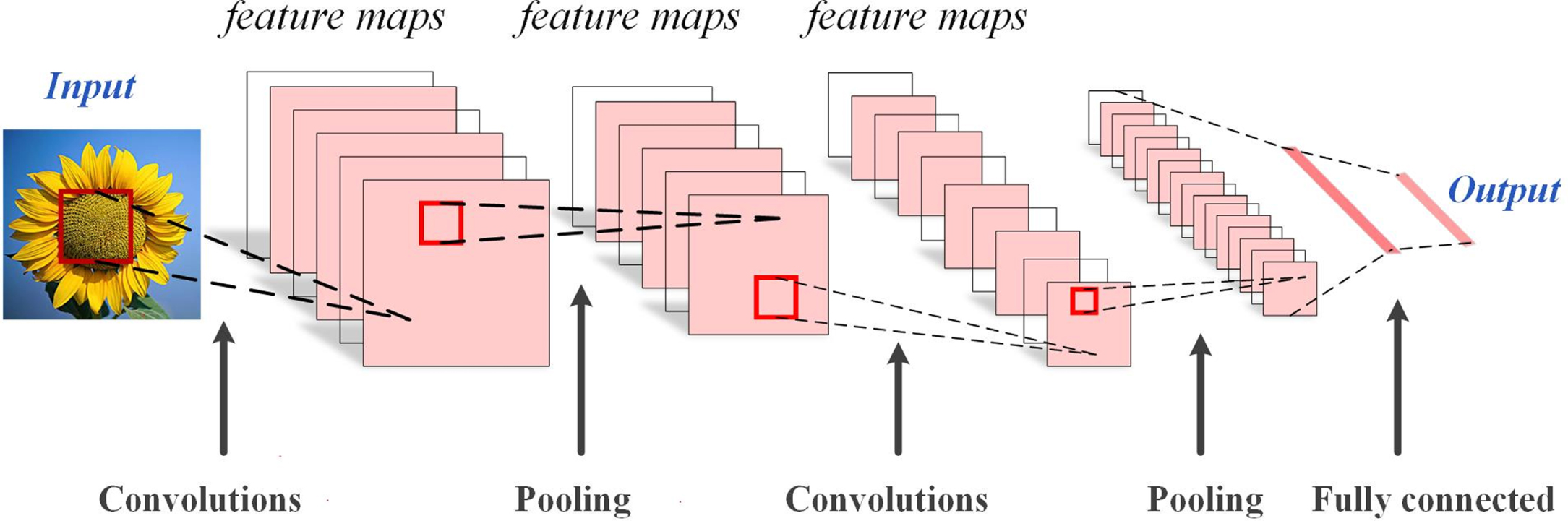
The basic CNN architecture.
Convolutional layer. As the core layers in the CNN model, the convolutional layers employ most of the calculating tasks. The parameters of those layers are constructed based on a set of learnable filters (or kernels) and trainable bias. Specifically, the features learned from previous layers will be convolved with various convolution kernels, and then more abstract features will be extracted. The convolution result shows that the image is split into perceptrons, creating local receptive fields and compressing the perceptrons in feature maps. Let
After the above three layers, the fully connected layers are usually followed by an activation function such as softmax or sigmoid to conduct the classification tasks.
Vibration signals have been widely applied in the fault diagnosis field. The vibration monitoring technique does not interrupt the production and could obtain abundant high frequency and time-varying information. Generally, feature extraction of vibration signals can be discussed from the time, frequency, and time-frequency domains.
Various statistical features are investigated in the time domain to represent how the signal amplitude varies with time. However, time-domain features only reflect the characteristics of waveform changes, ignoring the frequency-related information. Frequency domain methods extract features based on frequency analysis. Among these methods, the fast Fourier transform (FFT) is viewed as the most popular and effective technique [26]. Also, amplitude spectrum [27], power spectrum [28] and cepstrum [28] are extensively used in frequency-domain analysis. However, the frequency-domain techniques perform poorly in the analysis of non-stationary signals. For non-stationary signals, time-frequency analysis such as wavelet transform (WT) and empirical mode decomposition (EMD) performs as an effective method to extract information from both the time domain and frequency domain. However, there also exist drawbacks to these methods. For example, the selection of mother wavelet functions and wavelet decomposition in WT highly depends on manual experience, and the fitting errors and end effects caused by Hilbert transform in EMD could not be solved properly.
Considering the pros and cons of feature extraction methods from different domains, researchers have started to extract multi-domain features for fault diagnosis. Xu et al. [29] proposed a hybrid approach of multi-domain feature extraction, feature selection and cost-sensitive learning method for fault classification of rotating equipment. Yan et al. presented [30] a novel model based on multi-domain indicators to conduct different fault pattern identification of rolling bearing.
Proposed formulation for fault diagnosis
In this section, a novel DL-based diagnosis method for bearing diagnosis is developed. The multi-domain features are utilized to conduct image representation for the first time, and then the generated images are fed into a CNN model for classification.
Image representation
The CNN model is most commonly used in image classification. Hence, the first concern in this study is to construct images using the obtained multi-domain features. Assume that the features from three domains can be summarized as
Prior to the image mapping, the Φ needs to undergo normalization to bring all values into the range [0,1], which is given by
This square matrix c* can be then mapped into a color image according to RGB transformation. Based on the discussion above, a vibration signal can be skillfully transformed into an image with multi-domain feature information.
In this section, a new CNN model is proposed to extract features from the input images. Inspired by the classic LeNet-5, the architecture of the proposed CNN model in this study is made up of two convolutional layers, two maxing pooling layers, three fully connected layers and one Softmax layer. In addition, the batch-normalization technology is applied in each convolutional and maxing pooling layer in order to reduce overfitting and enhance learning rates. More detailed information about this CNN is shown in Fig. 2 and Table 1.
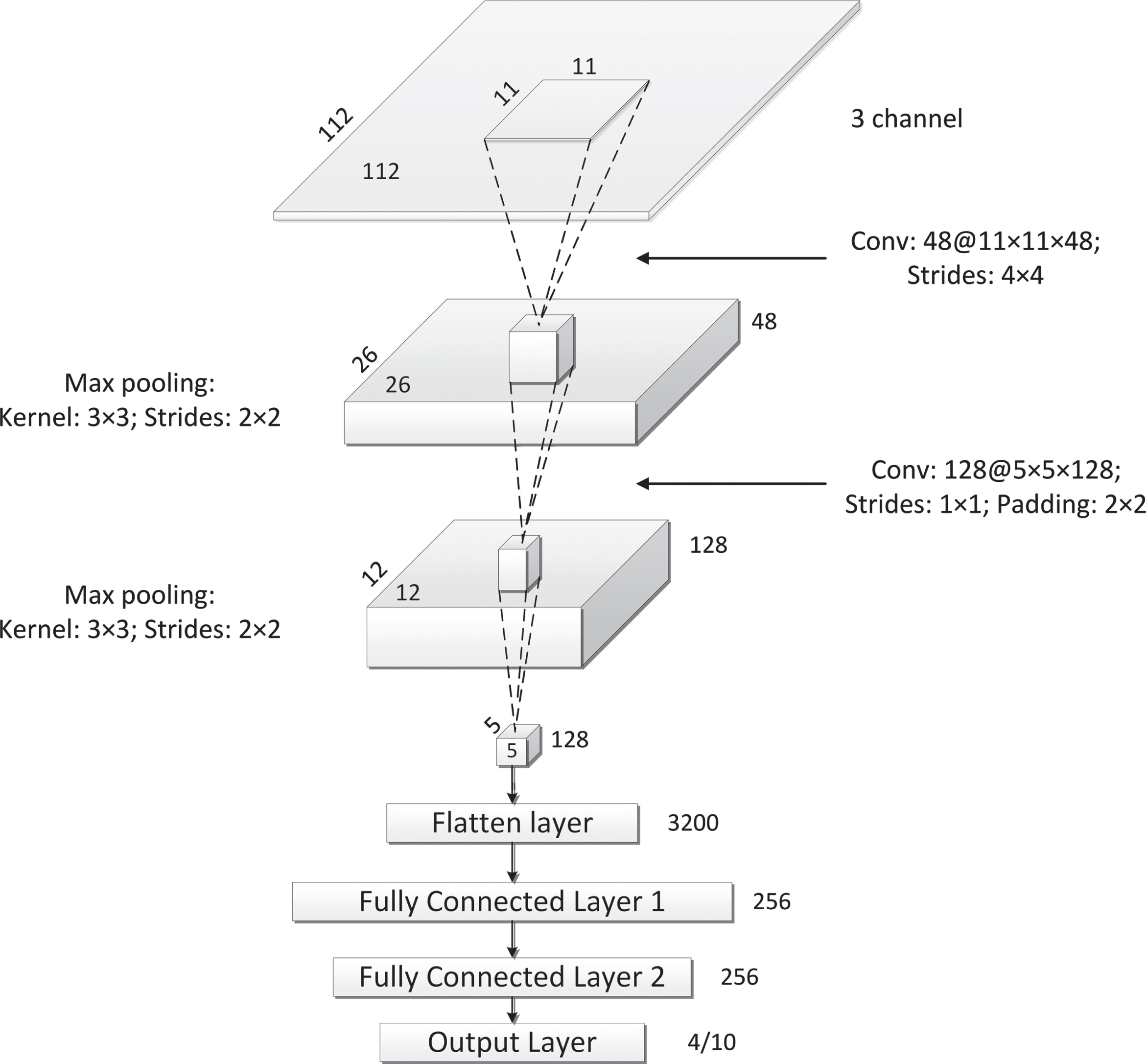
The proposed CNN architecture.
The details of the proposed CNN architecture
The size of the feature map is 112×112×3 in the input layer, and the output size of each layer is calculated as,
The hidden layer of the CNN architecture is divided into three stages. In the first stage, the 1st convolutional layer’s kernel size is set as a large number in order to decrease the noise of features. The 1st convolutional layer consists of 48 kernels with the size of 11×11×3, and these kernels are used at stride of 4×4 pixels in the horizonal and vertical direction. The 1st max pooling layer is made up of 48 feature maps with the size of 3×3. Furthermore, the batch normalization layer is placed between convolutional and maxing pooling layers. The second stage is similar to the first stage. However, the 2nd convolutional layer consists of 128 feature maps of 5×5 size, followed by 2nd max pooling layer of 128 feature maps of 3×3 size. The last stage consists of two fully connected layers of 256 features. Finally, the last layers are softmax layer of 10 or 4 classes. The new CNN model has fewer layers and parameters, achieving faster feature extraction and less computing consumption.
The presented study focuses on the validity of bearing fault classification using DL methods, and further discusses its performance compared with traditional methods. For this purpose, a new diagnosis framework is proposed. As seen in Fig. 3, the vibration signals measured from bearings are segmented into data samples, and then multi-domain features are extracted to obtain comprehensive fault information. According to section 3.1, various feature values are used to construct a square matrix, and then this matrix transforms into an image. This image representation contains more comprehensive vibration information from multiple domains. At last, the extracted images are fed into an ANN model to carry out classification tasks and status evaluation.
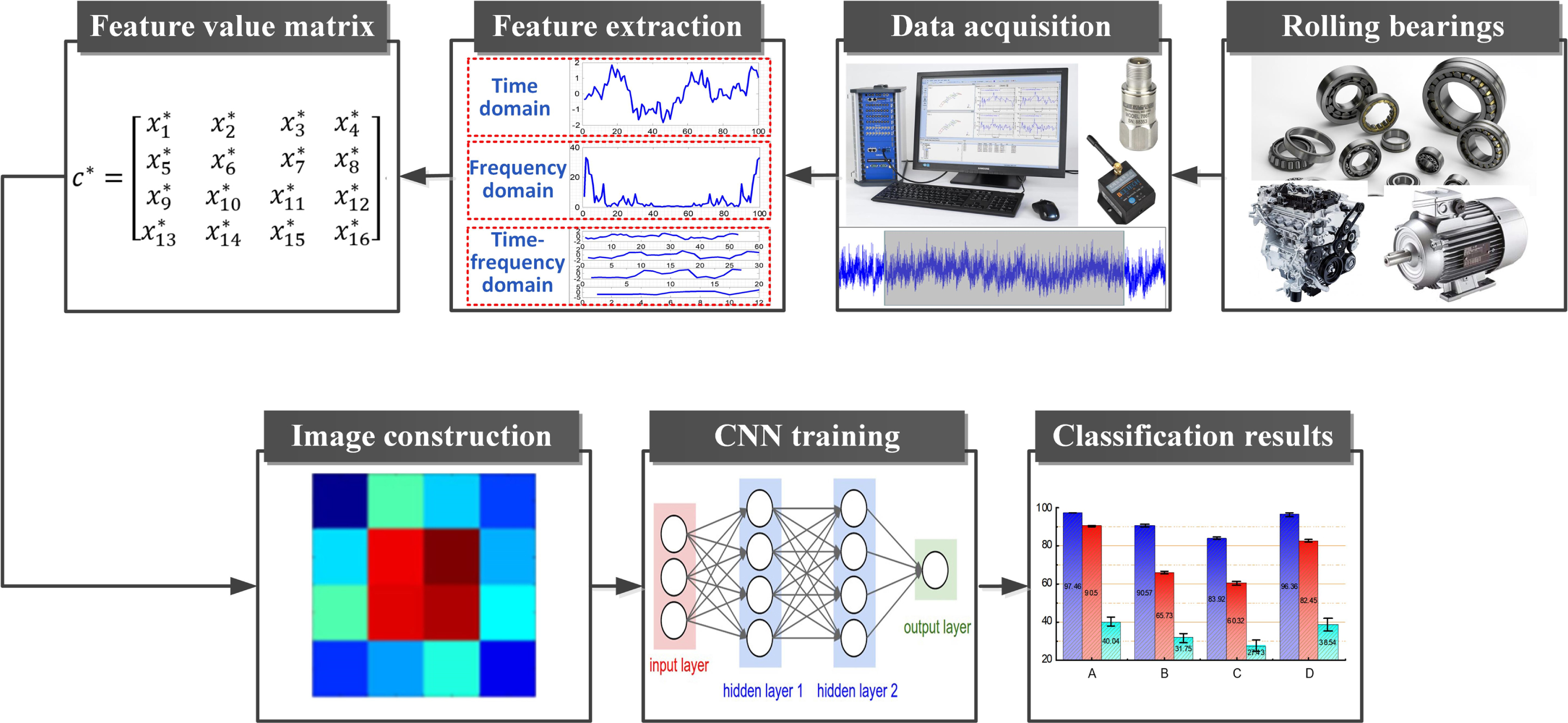
The proposed machinery diagnosis framework based on images and CNN.
Experiment setup and data description
The experimental data of rolling bearings applied in this study come from the public Case Western Reserve University (CWRU) bearing data center. As seen in Fig. 4, the test rig mainly consists of an induction motor, a transducer and a dynamometer. The vibration signals are collected by an accelerometer located at the driven end of the motor with a sampling frequency of 12,000 Hz. The deep groove ball bearings (6205-2RS JEM SKF) were seeded with signal point faults using electro-discharge machining (EDM). In addition to the normal condition (NC), the faults from 0.007 to 0.040 inches in diameter were also introduced to generate other three types of faults including inner-race faults (IFs), outer-race faults (OFs) and ball faults (BFs).
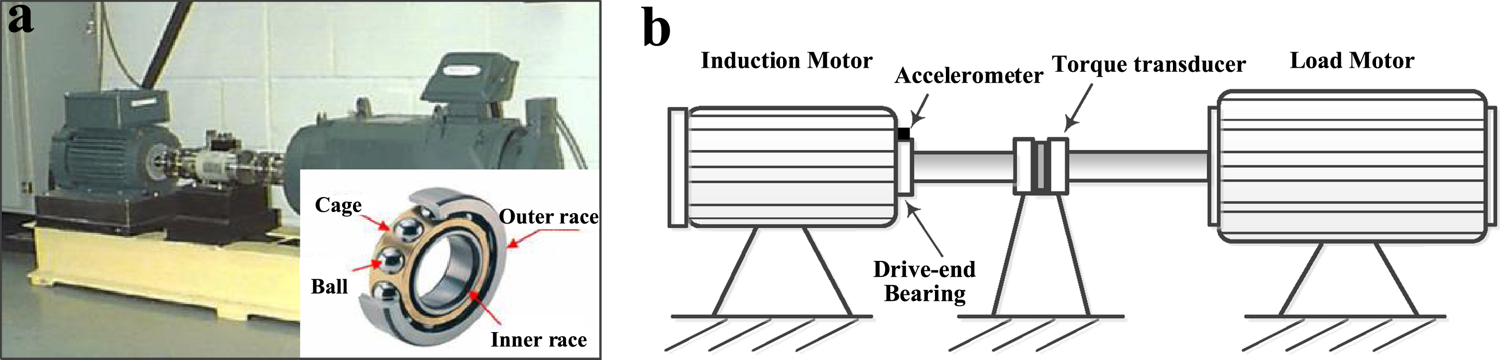
The CWRU bearing fault test rig and its schematic diagram [1].
A series of experiments are conducted on the rolling bearings to verify the validity of the presented approach. Four data subsets from CWRU bearing fault data are utilized, as shown in Table 2. Each data set discusses the classification of four types of faults. In the data set A, the incipient faults are employed, and the training and testing data are the bearing faults with fault diameters of 0.007 inches. The number of training and testing samples is relatively small. This experiment is to investigate the effectiveness of the presented method considering incipient faults under the condition of limited data samples. In data set B, the fault data with diameters of 0.014 inches is discussed. A small number of samples are used for training, while a relatively large number of samples are employed for testing. The purpose of this arrangement is to discuss the CNN generalization ability using a small number of samples. In data set C, the severe fault data with diameters of 0.021 inches is introduced. The sample set is organized as case B, but the numbers of training and testing are inverse to the case B. This is to assess the classification performance in the case of a large number of training samples. For further discussion, 10 sub-datasets including different defects with fault diameters of 0.007, 0.014 and 0.021 inches are employed in data set D. The ratio of training samples to testing samples is 7:3. This experiment is carried out to investigate the severe grades of faults.
Description of the four classification datasets
In this section, 25 features (14 time-domain features; 8 frequency-domain features; 3 time-frequency domain features) are extracted to conduct the image representation. In the time-frequency domain, the Empirical Mode Decomposition (EMD), Lempel-Ziv complexity and Wavelet Transform (WT) are introduced to extract features. The vibration signals are decomposed into eight Intrinsic Mode functions (IMFs) through EMD. The energy summation and the Lempel-Ziv complexity summation of the first five IMFs, are computed as two time-frequency features. Besides, the signals are decomposed into eight levels based on WT using the db4 wavelet packets. Similarly, the wavelet packet energy of the first five layers is added as the third time-frequency feature. These multi-domain features are listed in Appendix A.
The 25 features show the characteristics of vibration signals from different perspectives. However, some feature values (e.g. the FC, RMSF, MSF, etc.) are significantly larger than others. Thus, the relatively small original feature values will approach zero after normalization, leading to an indistinct pixel display in the transformed images. To address this issue, a weighting coefficient matrices is introduced to multiply by the original n × n feature matrix, as shown the Eq. 9. This data pre-processing aims to narrow the difference of magnitude order of original feature values and enhance the image representation.
Based on the above analysis, the c′ becomes a 5 × 5 square matrix. It can then be transformed into a pixel image by RGB color expression, where each element in the matrix corresponds to a color piece in the image. According to Eq. 9, the images from the data set D in Table 2 are listed in Fig. 5. Each image involves 25 squares corresponding to 25 normalized features.
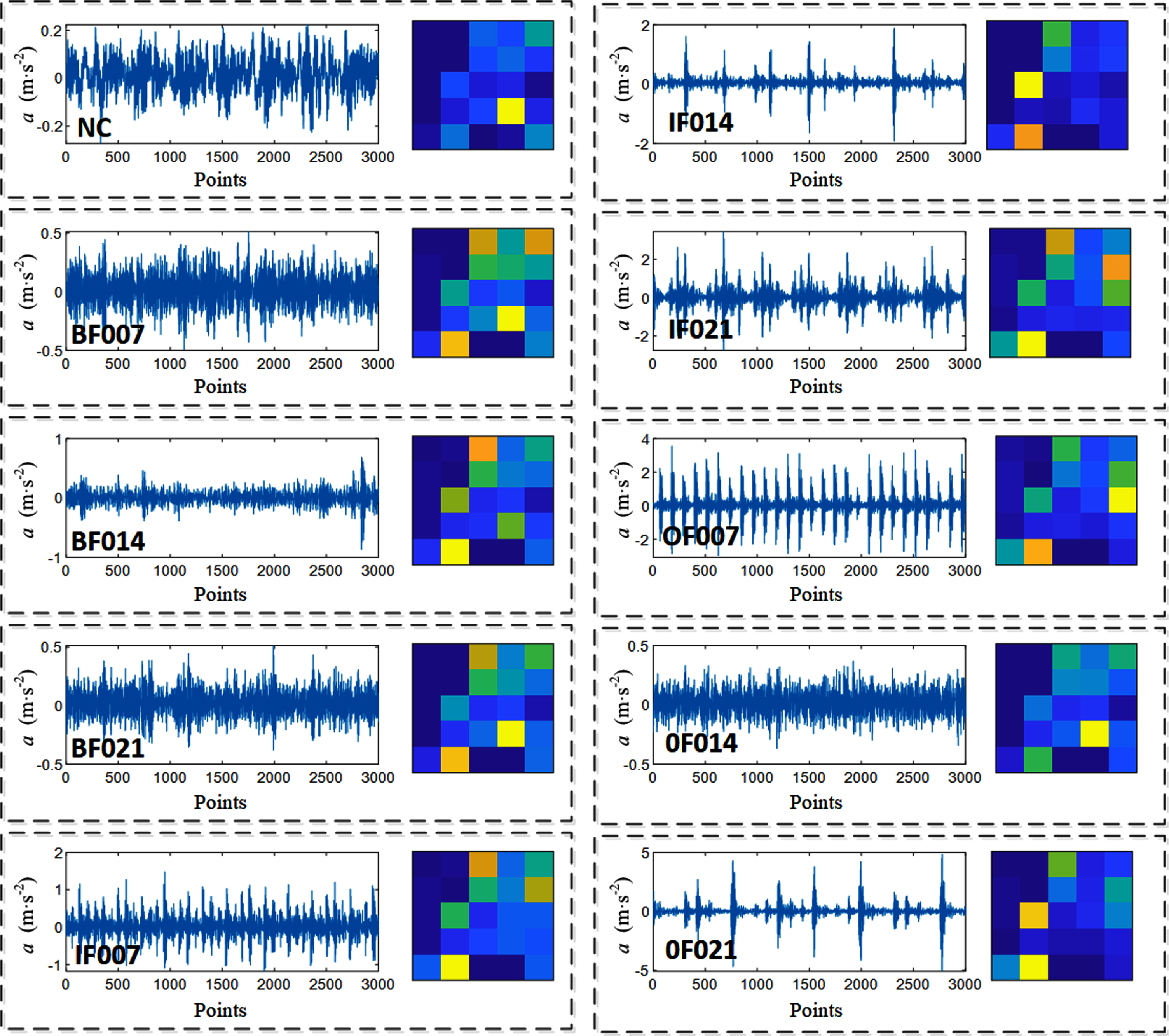
Image representation of the vibration signals from data set D in Table 2.
From these images, it is observed that there is a clear visual difference among these images. Taking the images of IF014 and OF021 as an example, the vibration waveforms of these two signals are very similar overall except for the vibration amplitude. However, the corresponding images have a noticeable difference related to the particular color piece. This difference implicates the potential effectiveness of the proposed image representation.
The datasets A-D classification results using the proposed method and two state-of-the-art CNN-based methods (best values are highlighted in bold)
The presented CNN-based fault diagnosis framework using images is verified through the experiments described in Table 2, and the classification results are summarized in Tables 3–4 in the form of confusion matrices. Generally, the overall classification result is quite impressive and the accuracy is up to 99.79%. The classification rate of set A is 100%, since this is a relatively simple classification task with a small number of training and testing samples. This perfect result demonstrates the proposed CNN-based fault diagnosis method works well in terms of incipient faults. For sets B and C, the data from two different severe grades of faults are investigated. The classification rates with both 100% are pretty satisfactory, implying that the presented approach also performs quite well with the increase in fault damage. For set B, a small number of training samples can give a desirable outcome, indicating the proposed CNN model has a good generalization ability. For set D, more training and testing samples are investigated, which is beneficial for DL training. The classification rate of 99.63% declines slightly, because more fault types are considered in this case. However, the outcome is still satisfactory. Overall, these experiments demonstrate the effectiveness of the proposed CNN-based framework for fault diagnosis.
Confusion matrix of the classification results of the data sets A, B and C
Confusion matrix of the classification results of the data sets A, B and C
Confusion matrix of the classification results of the data sets D
To further verify the superiorities of the proposed method, five typical features used in bearing health assessment are selected from Appendix A to conduct the comparative experiments. They are RMS in the time domain, mean frequency and frequency variance in the frequency domain, and energy summation of IMFs and WT. Two typical classifiers in shadow learning including the support vector machine (SVM) and K-Nearest Neighbor (KNN) are employed. The experimental results are seen in Fig. 6.
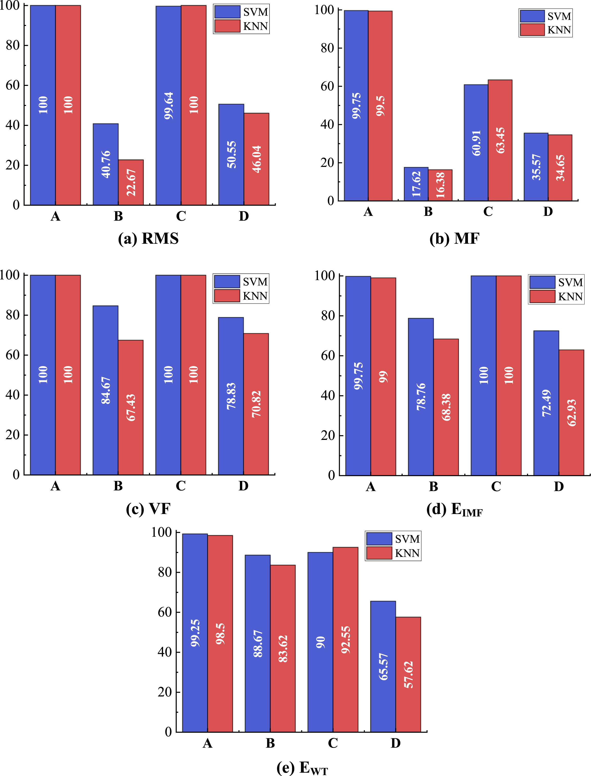
Classification accuracy using traditional features with different classifiers.
From Fig. 6, it is noted that the classification performance on set A is satisfactory regardless of the features. Furthermore, the SVM performs better than KNN, because parameter optimization is applied in SVM. It is also noted that the performance on set A is superior to set B, because more training samples are beneficial to modeling and learning in DL algorithms. Another important finding is that the time-frequency domain features yield the best performance, while the time domain features are worst-performing. It is clear that the time-frequency features reflect more comprehensive vibration information.
For further analysis, Fig. 7 gives a clear comparison results of traditional fault diagnosis approaches and the proposed method in this paper. It is noted that the presented CNN-based diagnostic scheme achieves impressive performance with a remarkable classification rate. Especially for set D, the excellent classification performance fully proves the effectiveness and the superiorities of the developed diagnostic scheme based on images and the CNN model. It is more effective to apply this new method to achieve end-to-end machinery fault diagnosis.
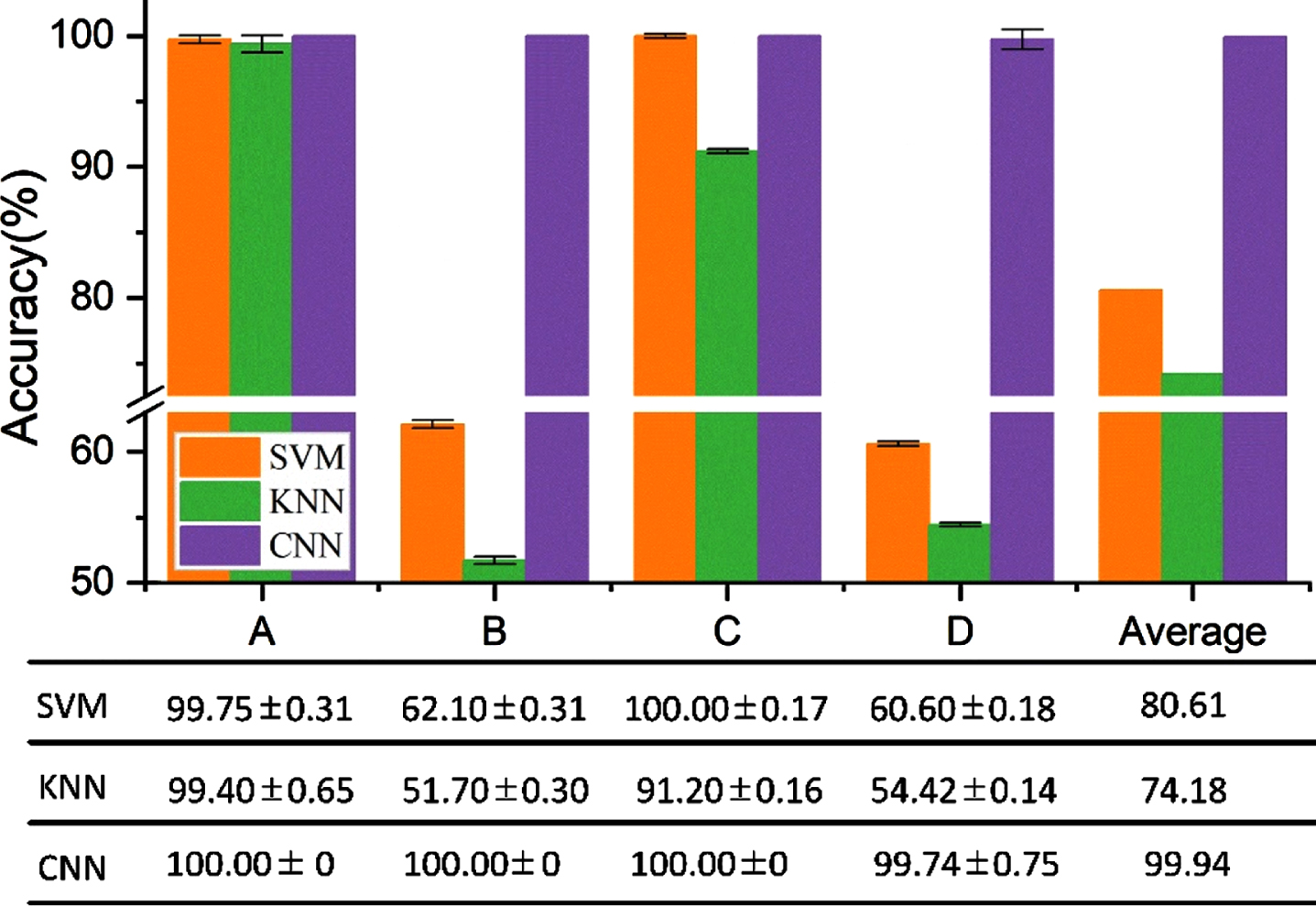
Summary comparison results using traditional fault diagnosis approaches and the proposed CNN based method.
In the last few years, more and more attention has been drawn to DL-based approaches applied to the fault diagnosis field, because the DL models can improve the diagnosis accuracy with the help of their multilayer nonlinear mapping ability. In this section, two state-of-the-art DL-based methods are introduced to carry out comparative experiments.
Zhang et al. proposed a 1-D CNN model using wide first-layer kernels (WDCNN) that can implement on raw signals without complex pre-processing [31]. In this method, wide kernels are used in the first convolutional layer to extract features and suppress high-frequency noise. The wide kernels are first used to extract features, and then successive small 3×1 kernels are applied to acquire better feature representation. However, the relatively shallow convolutional layers restrict the network’s ability to capture complex low-level features. For improvement, Shenfield et al. presented a novel dual-path DL network including a recurrent neural network path and a deep convolutional network path (RNN-WDCNN) [32]. This new method combines the features of RNN and CNN models to capture distant dependencies in time series data and suppress high-frequency noise in the input signals.
Comparative experiments are conducted using the data sets in Table 2, where four classification scenarios are discussed. Figure 5 shows the comparison classification results among the proposed model and two state-of-the-art DL-based models (WDCNN and RNN-WDCNN). Generally, it can be seen from these results that the proposed method performs best regardless of single classification accuracy or the average value. Especially for the first three classification tasks, the rate of 100% is impressive. In addition, the RNN-WDCNN performs slightly better than WDCNN, because the added RNN path in RNN-WDCNN aims to extract more locally situated features learned by the convolutional path and improve the final classification results. It is also observed that the ranking of classification accuracy from datasets A-D matches well with the conclusions drawn from Fig. 7. The CNN model is born for image processing, but the input to the RNN-WDCNN and WDCNN is 1-D vibration signals. This essentially leads to errors in the input data and training models. Overall, the proposed method is able to achieve good performance compared with other two state-of-the-art CNN-based fault diagnosis methods.
Conclusions
This paper focuses on image representation using multi-domain features, and proposes a new fault diagnosis method combining CNN with images. Unlike the traditional approaches using complicated hand-crafted features, this presented method only uses simple multi-domain features to construct images as the CNN input. This new image representation is able to capture complementary and rich diagnostic information from multi-scale domains. Besides, a modified CNN is proposed with the advantage of fewer training parameters and high computation efficiency. Combining CNN model and image representation, a new end-to-end fault diagnosis method is developed. Compared with the traditional feature extraction methods and state-of-the-art CNN-based methods, the proposed framework presents a good fault diagnosis capacity and performs better. Future work can be discussed on the effects of an imbalanced dataset and strong background noise. Also, we are considering developing a Matlab toolbox for multi-domain feature extraction where classic and state-of-the-art algorithms are embedded [33].
Footnotes
Acknowledgments
This work was supported by National Science Fund of China (grant number 12074403), China National Key Research and Development Plan (grant number 2016YFC0303700), and the China Scholarship Council (CSC) (grant number 201806440184). All the authors express heartfelt appreciation to editors and reviewers for their valuable comments and suggestions.
Appendix A. Traditional features in time,frequency and time-frequency domains
| Domain | Features | Expression | Features | Expression |
| Time | Variance | Standard deviation | ||
| RMS |
|
Average amplitude |
|
|
| Peak-to-peak value | P = max(x i ) - min(x i ) | RMS amplitude |
|
|
| Skewness |
|
Kurtosis |
|
|
| Waveform indicators |
|
Clearance factor |
|
|
| Impulse Factor |
|
Peak index |
|
|
| Variation coefficient |
|
Information entropy |
|
|
| ‘Frequency | Mean frequency |
|
Frequency center |
|
| Mean square frequency |
|
Frequency variance |
|
|
| Spectral skewness |
|
Spectral kurtosis |
|
|
| RMS frequency |
|
SD | ||
| frequency |
|
|||
| Time-frequency | IMF energy |
|
LZ complexity |
|
| Wavelet energy |
|