A method for efficient clustering of spatial data in network space

Abstract

Spatial clustering is one of the main techniques for spatial data mining and spatial data analysis. However, existing spatial clustering methods primarily focus on points distributed in planar space with the Euclidean distance measurement. Recently, NS-DBSCAN has been developed to perform clustering of spatial point events in Network Space based on a well-known clustering algorithm, named Density-Based Spatial Clustering of Applications with Noise (DBSCAN). The NS-DBSCAN algorithm has efficiently solved the problem of clustering network constrained spatial points. When compared to the NC_DT (Network-Constraint Delaunay Triangulation) clustering algorithm, the NS-DBSCAN algorithm efficiently solves the problem of clustering network constrained spatial points by visualizing the intrinsic clustering structure of spatial data by constructing density ordering charts. However, the main drawback of this algorithm is when the data are processed, objects that are not specifically categorized into types of clusters cannot be removed, which is undeniably a waste of time, particularly when the dataset is large. In an attempt to have this algorithm work with great efficiency, we thus recommend removing edges that are longer than the threshold and eliminating low-density points from the density ordering table when forming clusters and also take other effective techniques into consideration. In this paper, we develop a theorem to determine the maximum length of an edge in a road segment. Based on this theorem, an algorithm is proposed to greatly improve the performance of the density-based clustering algorithm in network space (NS-DBSCAN). Experiments using our proposed algorithm carried out in collaboration with Ho Chi Minh City, Vietnam yield the same results but shows an advantage of it over NS-DBSCAN in execution time.

Keywords

Spatial data mining spatial data clustering NS-DBSCAN network spatial analysis

1 Introduction

In recent years, the boom in big data has led to a rise in the use of Artificial Intelligence (AI) to address many challenges in the scientific community. Spatial big data attracts much attention from the academic community, business, industry, and governments, as it plays a primary role in addressing social, economic, and environmental issues of pressing importance [1]. The growth of spatial data, which plays a part in agricultural production, sustainable development, and human social development, is always speeding up. Not only are the size and volume of data immense, but the structure is also elaborate in terms of the abundance and depth of the contents. A spatial dataset is full of information and experience collection from geomatics that relates to Remote Sensing (RS), the Global Positioning System (GPS), and Geographic Information System (GIS). A wide variety of databases consist of electronic maps and planning networks from their infrastructures. As the collection of spatial data has grown exponentially and traditional methods fail to solve big data queries, the advent of more powerful techniques handling the processes of gathering, management, and transmission of data is now in urgent need. Spatial Data Mining (SDM) has thus been developed [2], especially with regard to the spatial data clustering technique.

The DBSCAN algorithm is a well-known method among a variety of types of clustering methods for detecting arbitrary shape clusters and noise elimination. Because of the significance of the DBSCAN algorithm, it has been researched thoroughly in order to develop a better version [3]. For example, the NS-DBSCAN clustering algorithm in the network space developed by Wang et al. includes a local shortest-path distance algorithm (LSPD) by gradually expanding from a central point to its adjacent vertex.

Moreover, the NS-DBSCAN algorithm creates favorable conditions to define the parameter MinPts by visualizing the density distribution of event points with the density order chart. However, due to the time-consuming clustering process, we propose solutions to reduce the time required by the NS-DBSCAN algorithm. Firstly, when data is set remove edges whose length exceeds eps because the path with a maximum length of eps definitely does not contain edges exceeding eps. This helps because the algorithm does not need to check the edges with a length greater than eps. Secondly, when building the density ordering table, we propose not including low-density points to reduce the time needed to check these points in the step of forming clusters. Thirdly, we optimize Algorithm 1 to reduce the number of calculations needed, eliminate the sort operation in Algorithm 2, and remove the noise identification part from Algorithm 3. The points that do not belong to any cluster will be considered as noise. If we are not interested in identifying noise, there will be no need to spend time to determine these points. This improvement is a step forward from the original algorithm, which can wrongly identify noise (while it’s supposed to be a border point) when the center point is not the core point.

The rest of this paper is organized as follows: In Section 2, related works are presented. Next, Section 3 presents a theorem for the early elimination of edges whose length exceeds the eps threshold and an improved algorithm based on this theorem. Section 4 then gives experimental results and evaluates the effectiveness of the proposed algorithm. Finally, Section 5 concludes the paper with a discussion on ongoing works.

2 Related works

In this section, current and previous studies in knowledge exploration and spatial data mining are presented. Spatial data plays an essential role in helping to detect geographic interdependence in networks and exploiting spatial data to detect relationships that exist in spatial databases. More and more studies are focused on discovering useful knowledge from large and complex spatial databases, and there are many algorithms that discover meaningful and useful knowledge from such databases.

Spatial data mining includes many different methods, such as knowledge discovery, clustering, aggregate proximity measuring, and spatial association rules, with some of the following objectives: understanding spatial data, discovering spatial relationships and relationships between spatial data and no n-spatial data, building spatial knowledge bases, reorganizing spatial database arrangement, and optimizing space queries. A crucial challenge to spatial data mining is the exploration of efficient spatial data mining techniques. As with non-spatial data, humans cannot manually analyze the enormous and complex spatial data that is now being collected. Therefore, spatial data mining algorithms are increasingly important, especially spatial data clustering algorithms.

Clustering analysis is used to identify clusters embedded in the data, where a cluster is a collection of data objects that are ‘similar’ to one another. Similarity can be expressed by distance functions, specified by users or experts. A good clustering method produces high quality clusters to ensure that the inter-cluster similarity is low and the intra-cluster similarity is high. For example, one may cluster the houses in an area according to their house category, floor area, and geographical locations. Clustering is a common technique for statistical data analysis which is used in many fields, including machine learning, data mining, pattern recognition, image analysis and bioinformatics. Clustering is the process of grouping similar objects into different groups, or more precisely, it is the partition of a dataset into subsets so the data in each subset is placed there according to defined distance measures.

The clustering problem has the aim of partitioning a set of data points into non-overlapping subsets. In the past few decades, many efficient clustering algorithms have been developed [4].

The clustering methods are classified into the following categories:

Partitioning: partition the data set of n elements into k clusters, such as: K-means, k-medoids [5]. Iterative clustering operations are performed by constantly updating central cluster points to stabilize the within-cluster variance. Partition-based methods need users to assign the number of clusters.

Hierarchical: Hierarchical clustering involves creating clusters that have a predetermined ordering from top to bottom, such as Balanced Iterative Reducing and Clustering using Hierarchies (BIRCH) [6], AGNES (Agglomerative Nesting), CURE (Clustering Using Representatives) [7], and so on. These methods are either agglomerative or divisive. Agglomerative methods begin with n clusters. In each step, two clusters are chosen and merged. This process continues until all objects are clustered into one group. Divisive methods begin by putting all objects in one cluster. In each step, a cluster is chosen and split into two. This process continues until n clusters are produced [8].

Density-based: Density-based clustering is an unsupervised learning method to classify high density points. Clusters are separated by regions of low density points such as DBSCAN [9], OPTICS (Ordering Points To Identify the Clustering Structure) [10], DENCLUE (Density-based Clustering) [11], ADCN (Anisotropic Density-based Clustering for discovering spatial point patterns with Noise) [12], CLARANS [8] and so on. In density-based clustering algorithms, clusters are high-density data regions divided by low-density regions. A cluster identified by density-based approaches can have arbitrary shapes. In addition, these approaches can handle noise very effectively. The majority of clustering algorithms based on density have been improved to apply to the spatial clustering algorithm [13]. Clustering by fast searching and finding of density peaks (CFDP) is a novel clustering algorithm based on density first proposed by Rodriguez and published in Science in 2014. The CFDP algorithm is based on the idea that cluster centers are characterized by a higher density than their neighbors, and by a relatively large distance from points with higher densities. However, because the CFDP algorithm still has some defects, many improvements have been proposed. The clustering algorithm named constraint-based clustering by fast search and find of density peaks (CCFDP) was proposed to solve the problem of CFDP: CFDP’s performance is quite sensitive to parameter selection, and relies on prior knowledge [14]. CFDP employs the clear neighborhood relations to calculate local density, so it cannot identify the neighborhood membership of different values of points from the distance of points, and it is impossible to accurately cluster the data of the multi-density peak. The fuzzy neighborhood density peak clustering algorithm (F-DPC) was proposed to address this shortcoming: novel local density is defined by the fuzzy neighborhood relationship [15]. The incremental variant of CFS (clustering by fast search) with multiple representatives (ICFSMR) also extended clustering using the fast searching and finding of density peaks method to process large dynamic data [16]. An adaptive core fusion-based density peak clustering (CFDPC) method is used for detecting clusters in any shape and density adaptively [17]. Kathia et al. also proposed an approach to automatically determine cluster centers by detecting gaps between data points in a one-dimensional version of a decision graph [18].

Grid-based: Grid-based clustering algorithms quantize clustered spaces into a finite number of cells to form a grid structure. Clustering is performed by identifying cells that contain more than a dense number of points and connecting these dense cells to form clusters. The processing time of these algorithms is fast because it usually does not depend on the number of data objects but on the grid’s size. Some of the grid-based methods are GRIDCLUS [19], GDILC [20], and WaveCluster [21], among others.

Model-based: This clustering method is often based on statistical theory or intelligent calculation tools [22], such as EM (Expectation-Maximization) [23], SOM (self-organization map) [24], and so on.

The ANN-based approach to clustering is presented in [25]. Baglietto and et al. applied a variant of the ‘mean-shift’ algorithm to density-based clustering in the state space [26]. Deep neural network-based clustering technique for secure Industrial Internet of Things (IIoT) has also been proposed based on power demand, and this ensures the security of data information in IIoT-based applications [27].

Bhattacharjee and et al. surveyed various density based clustering algorithms (DBCLAs) over last two decades along with their classification [28]. This paper studied as many as thirty-two DBCLAs and presented the related applications.

Improved versions of the DBSCAN algorithm are also proposed. DDNFC is a double-density clustering method based on the Nearest-to-First-in strategy to overcome the high error rate situation when clustering datasets with mixed density clusters [29]. The study presented in [30] uses unsupervised classification algorithms of K-means and PCA and supervised classification algorithms of LDA and DBSCAN for rice image classification. NG-DBSCAN is an approximate density-based clustering algorithm that operates on arbitrary data and any symmetric distance measure [31]. DBSCAN (AA-DBSCAN) and kAA-DBSCAN have clustering performances similar to those of existing algorithms for finding clusters with varying densities, while significantly reducing the running time required to perform clustering [32]. DBSCAN++, a modified version of DBSCAN is proposed in [33] that only computes the density estimates for a subset m of the n points in the original dataset.

3 NS-DBSCAND algorithm

Definition 1. [3] Neighborhood eps of point p (eps-neighborhood) is the set of points within eps distance from point p. Notation: N _ eps (p).

Definition 2. (The density of p) [3] The number of vertices in the set of neighboring points of p, |N _ eps (p) |, is defined as the density of vertex p. Notation: Density (p).

Definition 3. (Basic expansion) [3] Basic expansion is the movement from vertex A to vertex B on the same edge. A is called the starting vertex and B is the ending vertex. The edge connecting these two vertices is called the expansion path. The length or distance of an expansion path is the weight (length) of the edge between the two vertices.

Definition 4. (Core points) [3] Core points are event points having a density that is greater than the minimal density MinPts. The set of its neighbor points within the distance of the eps (N _ eps ()) is called the border points.

The idea of the NS-DBSCAN algorithm

The algorithm is formed from the basic idea that adjacent points have similar densities. Therefore, the authors have proposed building the density ordering table starting from a point (called the central point), then continuing by adding the neighbors (called border points) of a high-density point (≥MinPts, called core point) into the density ordering table so the density of adjacent points is in descending order. The process is repeated for all vertices as the central vertices.

Points near each other tend to be similar in density and will be placed close to each other in the density ordering table. The density ordering table can be displayed as a graph. This chart (Fig. 1) shows hills of different sizes that correspond to implicit clusters [3].

Fig. 1

The points close to each other in space are similar in density and close to each other in the density ordering table/graph ([3]).

Expanded from the DBSCAN algorithm, NS-DBSCAN is composed of two main steps with the following three algorithms:

Step 1 –Generating the density ordering table using the following algorithms:

Algorithm 1 –Local shortest-path distance (LSPD) algorithm defines eps-neighbors, the density of an event point.

Algorithm 2 –Generating density ordering with the densities of event points by one parameter eps.

Step 2 –Forming clusters by using Algorithm 3. Based on the density ordering chart, this step determines the value for the MinPts parameter. Adjacent and dense vertices are grouped into the same cluster.

The step of generating density ordering is to determine the eps-neighborhood for all event points by calculating the shortest path length of p to the remaining points within distance eps. The point with the shortest path length to p that does not exceed eps is the neighbor of p.

The set of points are neighbors of a central vertex s in the range eps that is determined by Algorithm 1 –Local shortest-path distance (LSPD):

Notations:

The shortest-path distance from a central vertex to each point e is d (e).

The length or weight of the edge from s to e is W (s, e).

Assigning the distance from the central vertex to s to 0and the distance from the central vertex to the other vertices to ∞.

Finding the eps-neighborhood of s by basic expansion from s to its adjacent vertex e along the edge so the sum of the distance from the central vertex to s and the length of edge from s to e is less than eps. Similarly, the basic expansion is continued from the new vertices until all expansion paths are blocked.

After each basic expansion from s to e, the d (e) is updated using the formula: d (e) = d (s) + W (s, e).

The purpose of the basic expansion is to minimize the distance from a central vertex to every ending vertex e with the eps constraint. If basic expansion does not reduce the distance d (e) or the d (e) exceeds eps, this expansion path would be blocked.

In Fig. 2, if d (P₁) + W (P₁, P₂) ≥ d (P₂) or d (P₁) + W (P₁, P₂) > eps, the expansion path P₁ - P₂ would be blocked. The set N _ eps (p) contains all points that are basic expansions in turn from p that is the neighbor eps of p. The number of points in the set N _ eps is called the density of p.

Fig. 2

Basic expansion from the start vertex to the end vertex [3].

The authors have proposed the local shortest-path distance (LSPD) algorithm. The distribution of event points is visualized to help precisely determine the two parameters of eps and MinPts. However, in the process of basic expansion within the distance of eps with Algorithm 1 (LSPD algorithm), a check on whether the adjacent vertices with edges exceeding the distance of eps is still made. This is unnecessary because edges whose length exceeds eps can not exist in a segment with a maximum length of eps, and the process stops expanding from P₁ to P₂ when d (P₁) + W (P₁, P₂) ≥ d (P₂) or d (P₁) + W (P₁, P₂) > eps. In fact, the expansion stops functioning in conditions of length = eps. This means that the stopping conditions should be d (P₁) + W (P₁, P₂) ≥ d (P₂) or d (P₁) + W (P₁, P₂) ≥ eps to reduce the processing time. In addition, the step of forming clusters will browse through all the points in the density ordering table. Factually, there is no need to browse points that are not core points to further reduce the processing time.

4 Proposal to improve the NS-DBSCAND algorithm

The following definitions and notations are related to the proposed method:

Definition 4. [34] A graph G is defined as a pair of sets of edges V and sets of vertices E . Notation: G = (V, E). An edge is a pair of vertices (s, e) or (e, s) such that s, e ∈ V.

Definition 5. [34] A weighted graph G consists of three components: the set of vertices V, the set of edges E and the set of values representing the length of the edges W. Notation: G = (V, E, W).

Definition 6. An undirected graph G = (V, E, W), the path from P₀ to P_n is represented as a sequence of vertices P₀, P₁, P₂, …, P_n-1, P_n ∈ V.

The path can also be expressed as a sequence of edges: (P₀P₁) , (P₀P₁) , …, (P_n-1P_n) ∈ E.

There could be several paths or no path at all between the two points. When there are several paths between two points, we can determine the shortest path.

Definition 7. The length of the path from point P₀ to point P_n passing through points P₁, P₂, …, P_n-1 ∈ V has the value of the sum length of all segments of the path. $\begin{matrix} d (P_{0}, P_{n}) = W (P_{0}, P_{1}) + W (P_{1}, P_{2}) \\ + \dots + W (P_{n - 1}, P_{n}) \end{matrix}$

Definition 8. [34] The shortest path from point P₁ to point P_n is the path from P_o to P_n with the shortest length.

Theorem 1. A path with a maximum length of eps cannot contain an edge that has a weight greater than eps.

Proof. Let eps be the sum of the path length from e₁ to e_n: e₁, e₂, …, e_n-1, e_n and d (e_i) is the length of e_i. There is at least one edge e_i such that: $eps = d (e_{1}) + d (e_{2}) + \dots + d (e_{n}) = \sum_{i = 1}^{n} d (e_{i})$ (1)

To prove this: There is no edge e_i longer than eps.

If e_k exists with 1 ≤ k ≤ n, k ∈ N so: d (e_k) > eps. $Since d (e_{k}) > eps, deduce : eps - d (e_{k}) < 0$ (2)

But according to formula (1): $eps - \sum_{i = 1}^{n} d (e_{i}) = 0$ (3) $Replace d (e_{k}) to (3) : eps - d (e_{k}) = 0$ (4)

(4) contradicts (2).

Therefore, the initial assumption must be false. That is, there is no edge whose length is larger than eps.

Applying Theorem 1, the first improvement is to remove edges whose length exceeds esp since it certainly does not expand in a basic way to adjacent vertices whose edge length is greater than eps.

As such, the algorithm does not need to check the edges longer than eps, as shown in Algorithm 1, and this helps reduce the algorithm’s runtime several fold during the clustering process.

Proposition 1. The edge length is always greater than zero.

Applying Proposition 1, when the expansion path has reached eps, it does not perform a test operation for basic expansion anymore, and this reduces the basic expansion time for the points that have reached eps.

In Algorithm 2 –Constructing the density ordering table has two suggestions for the following enhancements:

When inserting a point in queue Q, it should be inserted in the designed descending order in a bid to keep the original order of the sequence. This helps reduce the time needed to sort the Q list in the loop.

When building the density ordering table, we propose not taking low density points into consideration to reduce the number of browsing points in the next step of forming clusters. A low-density point is one with a density that is less than the possible minimum value of MinPts. This helps reduce the number of scans through these points in the iteration statement of Algorithm 3 (line 1), which decreases the execution time. Thus, a heuristic is employed to determine the minimum value for MinPts threshold.

The minimum value of the MinPts parameter can be taken from the size of the data set (denoted as n), MinPts ≥ n + 1. The low value of MinPts = 1 does not make sense, as then every point on its own will already be a cluster. With MinPts ≤ 2, the result will be the same as with hierarchical clustering with the single link metric. Therefore, inPts must be at least 3 [35]. However, to get denser and more significant clusters, MinPts should be set with a larger value. In general, the recommended value for MinPts is n [36].

Devkota et al. noted that “many studies in the literature follow a trial-and-error approach with various values and compare the clustering results with the background knowledge of the study area in order to select some absolute values as the parameters (e.g., eps = 100 and MinPts = 10)” [37]. Birant et al. state that “the heuristic suggests MinPts ≈ ln (n) where n is the size of the database” [38]. So with the experimental dataset consisting of 10,352 points, we do not include points for which our densities are smaller than ln (10, 352) ≈ 9 in the density ordering table.

In Algorithm 3 - Cluster formation: Noise is identified during cluster formation since noise will be those points that do not belong to any cluster. That is, we do not execute lines 3 and 4 to determine noise. With regard to line 2, we also omit the check for event points that do not belong to noise. This helps remove three test operations in the loop at line 1. Therefore, the algorithm’s execution time is decreased.

The algorithms are summarized in the schematic diagrams of Figs. 3 –5.

Fig. 3

Flowchart of Algorithm 1.

Fig. 4

Flowchart of Algorithm 2.

Fig. 5

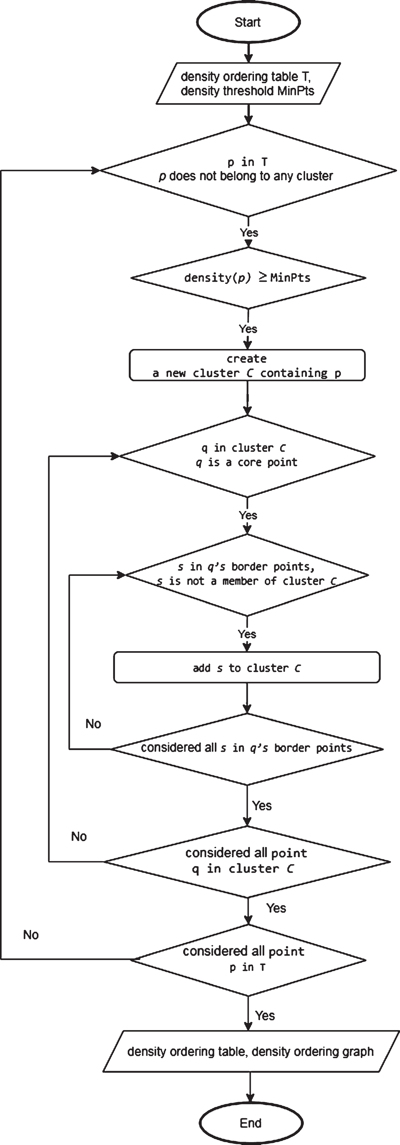
Flowchart of Algorithm 3.

Algorithm 1. Local shortest-path distance (LSPD):

Input: undirected planar graph N, central vertex cp, radius eps

Output: cp’s eps -neighbors N_ eps ( cp )

Original algorithm

Algorithm 1. Local shortest-path distance (LSPD)
(1) d (cp) =0, d (other vertices) =∞,
cp is inserted into a newly initiated queue Q;
(2) while Q is not empty do
(3) p is dequeued from Q;
(4) if p is an event vertex and not in N_eps(cp) then
(5) add p to N_eps(cp);
(6) end if
(7) for each vertex q adjacent to p do
//using theorem 1: decrease //
// number of adjacent points in this loop
(8) if d (p) < eps then //using Proposition 1
(9) if d (p) + W (p, q) < d (q) and d (p) + W (p, q) ≤ eps then
(10) d (q) = d (q) + W (p, q);
(11) if q is not in Q then
(12) q is enqueued to Q;
(13) end if
(14) end if
(15) end if
(16) end for
(17) end while

Line 8 shows that the algorithm still continues the test to carry out basic expansion when the distance has reached eps.

Improvements

When organizing data, we remove edges whose length exceeds eps because the path with a maximum length of eps definitely does not contain edges exceeding eps. That helps to decrease the number of adjacent points of the loop in line 7.

At the point where the length from the center point to it has reached the eps distance, we do not check to expand anymore: we stop the test operation after the vertices have reached eps.

Illustrations

In Fig. 3, assuming eps = 1, the central point was randomly selected as P₅. According to Algorithm 1, the neighborhood within the distance eps of P₅ (N _ eps (P₅)) is as follows:

Basic expansion from P₅ to vertices P₁ and P₈:

–Calculate d for P₁ and P₈:

+d (P₁) = d (P₅) + W (P₅, P₁) =0 + 0.5 = 0.5

+d (P₈) = d (P₅) + W (P₅, P₈) =0 + 0.5 = 0.5

The new values of d (P₁) and d (P₈) are smaller than their current d and less than eps, so P₅ is expanded to P₁ and P₈, meaning that P₁ and P₈ become the start vertex in the next expansion.

–For P₁: Continue to basically expand from P₁ to P₂ and P₁ to P₃, which gives:

d (P₂) = d (P₁) + W (P₁, P₂) =0.5 + 0.5 = 1 = eps

d (P₃) = d (P₁) + W (P₁, P₃) =0.5 + 0.5 = 1 = eps

–For P₈: Basically, expand from P₈ to P₄, P₈ to P₇ and P₈ to P₉.

+d (P₄) = d (P₈) + W (P₈, P₄) =1 = eps

+d (P₇) = d (P₈) + W (P₈, P₇) =1 = eps

+d (P₉) = d (P₈) + W (P₈, P₉) =1 = eps

Points P₂, P₃, P₄, P₇, P₉ have reached eps so we do not extend anymore and the conclusion could be: N _ eps (P₅) = {P₁, P₈, P₇, P₉, }. While the original algorithm still continues to expand: “The expansion continued with P₂, P₃, P₇, P₉ and P₄ as the start vertices until all the expansion paths were blocked” [3].

Algorithm 2. Generating Density Ordering

Input: undirected planar graph N, radius eps

Output: density ordering table, density ordering graph

Original algorithm

Algorithm 2. Generating Density Ordering
(1) initialize density ordering table;
(2) for each point p do
(3) if p is not in density ordering table then
(4) p is inserted into Q and get N _ eps (p) by LSPD algorithm;
(5) end if
(6) while Q is not empty do
(7) the first point q is dequeued from Q
(8) if density (q) ≥ ln (n) //n is number of event p
(9) write the density of q and N _ eps (q) ordering table;
(10) for each point q in N _ eps (q) do
(11) if q’s density is unknown then
(12) calculate its density by LSPD algorithm;
(13) end if
(14) if q is not in density ordering table nor in Q then
(15) add q into Q at the suitable location to make the
densities of the points in Q are from high to low
order: No need to sort Q
(16) end if
(17) end for
(18) end if
(19) end wile
(20) end for
(21) draw a density ordering graph according to the density
ordering table;

At line 13 and in the algorithm illustration of [3], the algorithm starts to sort Q after the data is inserted into Q.

The density ordering table is constructed containing all the points, including those that have a density of 0 and no neighbors at all. These points definitely do not belong to any cluster.

Improvements

When inserting a point into Q, we should insert it in descending order of density measurement to maintain the original order of the array so Q does not have to be reordered. Because putting the vertices into Q is correct in the sort order, the result is correct.

For sample data with 16 points, the points whose density is less than ln (16) ≈ 3 are not included in the density ordering table.

Illustrations

An empty table T is initialized. In order of names of the event points, P₁ is selected first, and compute N _ eps (P₁) = {P₅, P₂, P₄, P₈, P₃} and queue Q = {P₁}. Q is not empty. Take P₁ from Q and put the record {(ID: P₁; density: 5; N _ eps : {P₅, P₂, P₄, P₈, P₃}) into the density ordering table T.

The density of the points in the set of N _ eps (P₁) is calculated and put into the appropriate position of Qso Qhas an order of density from high to low:

N _ eps (P₅) = (P₁, P₈, P₉, P₇) → Q = {P₅}

N _ eps (P₂) = (P₃, P₄, P₁) → Q = {P₅, P₂}

N _ eps (P₄) = (P₂, P₁, P₃) → Q = {P₅, P₄, P₂}

N _ eps (P₈) = (P₅, P₉, P₁, P₇, P₆) → Q = {P₈, P₅, P₄, P₂}

N _ eps (P₃) = (P₂, P₄, P₁) → Q = {P₈, P₅, P₃, P₄, P₂}

Q = {P₈, P₅, P₃, P₄, P₂} with the corresponding density in descending order of 5, 4, 3, 3 and 3.

According to the original algorithm, if points in N _ eps (P₁) are put into Q in compliance with the order already used in N _ eps (P₁), the arrangement of those points will be Q = {P₅, P₂, P₄, P₈, P₃}. On the other hand, if points in Q are sorted according to the order of their densities from high to low, that is Q = {P₈, P₅, P₂, P₄, P₃} as in [3].

Then, take out the first point with a density that is bigger than or equal to 3 in Q (P₈) and put it in the density ordering table T. $\begin{matrix} T = {(P_{1}, 5, {P_{5}, P_{2}, P_{4}, P_{9}, P_{3}}), \\ (P_{8}, 5, {P_{5}, P_{9}, P_{1}, P_{7}, P_{6}})} \end{matrix}$

The density values of points P₇, P₉, and P₆ are calculated as 4, 3, and 3, respectively. The queue Q is updated to be {P₅, P₇, P₂, P₄, P₃, P₉, P₆}. Then, the first point in Q is removed from the queue to continue performing the above-mentioned operations until Q is empty. As a result, the order of points in T is P₁, P₈, P₅, P₇, P₂, P₄, P₃, P₉.

These are points related to P₁ in terms of neighbor relations for the distance eps.

Continue to consider points from P₂ to P₁₆. Points from P₂ to P₉ are already in the density ordering table.

Similar to P₁, we consider P₁₀: Q = {P₁₀}, N _ eps (P₁₀) = {P₁₁}. P₁₀ is not included in the density ordering table T because Density (P₁₀) =1. Similarly, Density (P₁₁) =1 so P₁₁ does not exist in T.

Continue with P₁₂: $Q = {P_{12}}, N_eps (P_{12}) = {P_{13}, P_{14}, P_{15}},$ $Density (P_{12}) = 3 .$

Add P₁₂ into the density ordering table T composed of points P₁, P₈, P₅, P₇, P₂, P₄, P₃, P₉} and P₁₂.

Doing the same as with P₁, we get the following T results: $\begin{matrix} T = & {(P_{1}, 5, {P_{5}, P_{2}, P_{4}, P_{8}, P_{3}}), \\ (P_{8}, 5, {P_{5}, P_{9}, P_{1}, P_{7}, P_{6}}), \\ (P_{5}, 4, {P_{1}, P_{8}, P_{9}, P_{7}}), \\ (P_{7}, 4, {P_{8}, P_{6}, P_{5}, P_{9}}), \\ (P_{2}, 3, {P_{3}, P_{4}, P_{1}}), \\ (P_{4}, 3, {P_{2}, P_{1}, P_{3}}), \\ (P_{3}, 3, {P_{2}, P_{4}, P_{1}}), \\ (P_{9}, 3, {P_{8}, P_{5}, P_{7}}), \end{matrix}$ $\begin{matrix} (P_{6}, 3, {P_{7}, P_{8}, P_{1}}), \\ (P_{12}, 3, {P_{13}, P_{14}, P_{15}}), \\ (P_{13}, 4, {P_{12}, P_{14}, P_{15}, P_{16}}), \\ (P_{14}, 4, {P_{13}, P_{12}, P_{15}, P_{16}}), \\ (P_{15}, 4, {P_{12}, P_{13}, P_{14}, P_{16}}), \\ (P_{16}, 3, {P_{13}, P_{14}, P_{15}}), \end{matrix}$

Compared to the original algorithm, there are both P₁₀ and P₁₁ before P₁₂. It takes some time to examine these points in the next step in forming clusters.

The density ordering graph of the road network in Fig. 6 is depicted in Fig. 7.

Fig. 6

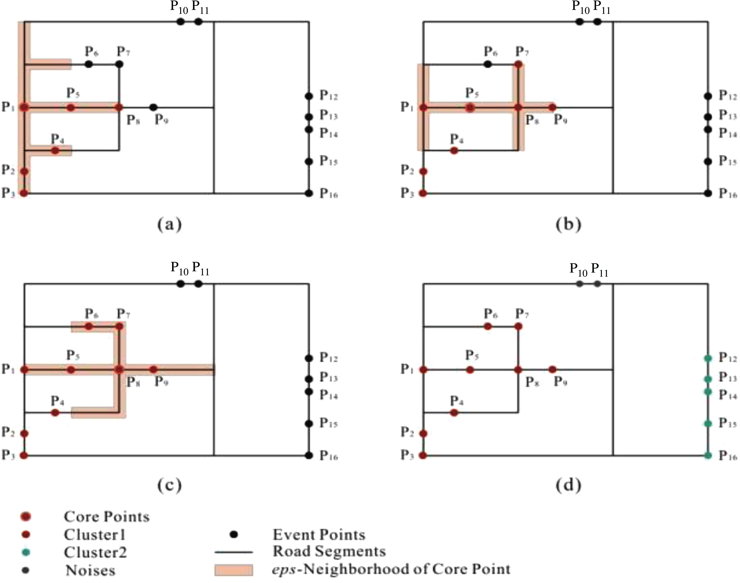
The border points of the core points are gradually put into the cluster: (a) P₅, P₂, P₄, P₈ and P₃ are put into cluster C₁ through P₁: (b) P₇ and P₉ are introduced into cluster C₁ through P₅: (c) P₈ brought P₆ to C₁: cluster C₂ is formed from simulation data set (d) [3].

Fig. 7

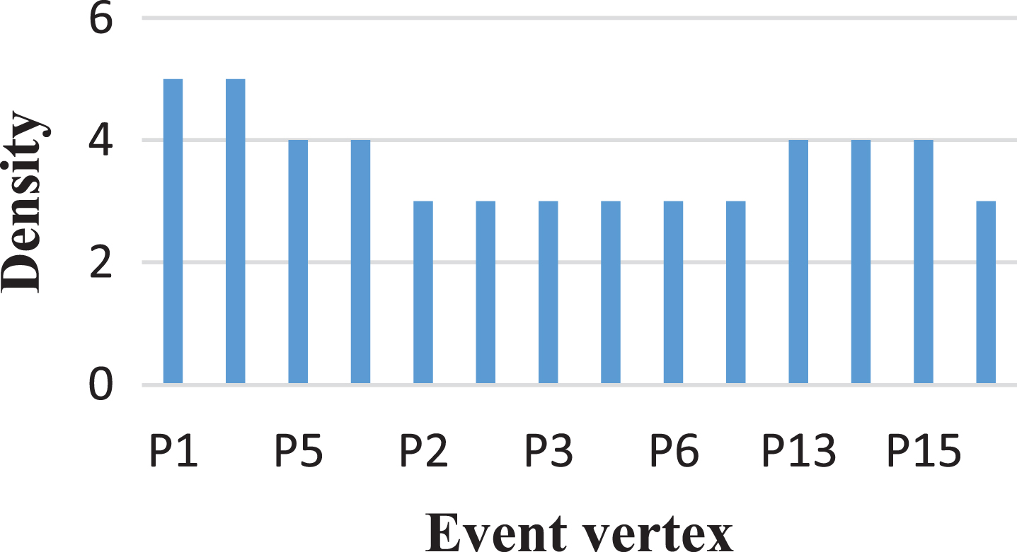
A density ordering graph of a simulated dataset.

Algorithm 3. Forming Clusters:

Building clusters: Initialize the cluster with core points and gradually add the border points into the cluster until no border points are added.

Input: density ordering table, density threshold MinPts

Output: density-based clusters

Original algorithm

Algorithm 3. Forming Clusters
(1) for each event point p in density ordering table do
(2) if p does not belong to any cluster then
(3) if the density of p is more than or equal MinPts then
(4) create a new cluster C containing p;
(5) end if
(6) for each point q in cluster C do
(7) if q is a core point then
(8) for each point s in q’s border points do
(9) if s is not a member of cluster C then
(10) add s to cluster C;
(11) end if
(12) end for
(13) end if
(14) end for
(15) end if
(16) end for

At line 2, the algorithm checks whether the event points belong to any clusters or sets of noise, lines 3 and 4 then continue evaluating the condition of points whose density is less than MinPts to assign those to noise.

The process of assessing whether points belong to any clusters or collections of noise in the for loop of line 1 costs time. Moreover, it is possible to wrongly assign border points whose density is less than MinPts to noise.

Improvements

Noise is not determined during the process of cluster formation. Noise is those points that do not belong to any clusters. That is, lines 3 and 4 do not need to be executed to determine noise. Moreover, the statement in line 2 also omits the check as to whether an event point belongs to the noise set. This helps remove three test operations in the loop of the line 1. Therefore, the algorithm execution time is decreased. We do not determine core points in the process of forming clusters, and the noise will be those points that do not belong to any clusters. That is, we do not execute lines 3 and 4 to determine noise. Moreover, the statement in line 2 also omits the check as to whether an event point belongs to the noise set.

Illustration

Considering eps = 1, MinPts = 4.

P₁ is selected as the core and P₁ does not in any clusters. Therefore, a new cluster, namely C₁, is created containing P₁. The border points of P₁ (N _ eps (P₁) = {P₅, P₂, P₄, P₈, P₃}) is added into C₁ so C₁ = {P₁, P₅, P₂, P₄, P₈, P₃} (Fig. 6a).

The next selected core point in C₁ is P₅. The set of P₅’s border points is {P₁, P₈P₇P₉}, where P₁ and P₈ ∈ C₁, P₇ and P₉ ∉ C₁, so P₇ and P₉ are added to C₁ (Fig. 6b), C₁ = {P₁, P₅, P₂, P₄, P₈, P₃, P₉, P₇, }. The density of P₂ and P₄ is 3, which is less than the value of MinPts (4), so no more points are added to C₁. Similarly, P₈ is the core point, so border points {P₅, P₉, P₁, P₇, P₆} are added to C₁ (Fig. 6c): $C_{1} = {P_{1}, P_{5}, P_{2}, P_{4}, P_{8}, P_{3}, P_{9}, P_{7}, P_{6}} .$

P₃, P₉ and P₆ are not core points.

P₇ is the core point but all its border points are {P₈, P₆, P₅, P₉}, which belong to C₁.

Finally, the cluster C₁ = {P₁, P₅, P₂, P₄, P₈, P₃, P₇, P₉, P₆} is formed.

Similarly, the algorithm assigns P₁₂ to P₁₆ for the new C₂ cluster.

The results of the clustering process are shown in Fig. 6d.

The original algorithm is capable of noise detection, and thus it marks P₁₀ and P₁₁ as noise.

5 Experiments

This section presents the experimental results of the original NS-DBSCAN algorithm and the proposed improved algorithm, thus evaluating the efficiency of the improved algorithm compared to the original one.

5.1 Dataset

The Open Street Map (OSM) provides an easy-to-access platform that allows free access to geographic information worldwide.

The information is gathered by many volunteers from around the world, collated on a central database and distributed in many digital formats. Although OSM does not have a strict quality control mechanism, analysis shows that information about OSM can be quite accurate, and the data obtained from OSM is good enough and comparable to authoritative data to some extent [39].

OSM provides many types of data, such as points, lines, and regions. Points often represent points such as supermarkets, restaurants, hotels, schools, and so on. Polylines are used to indicate roads such as roadways, waterways, and railways. Polygons represent regional features such as national administrative regions, parks or forests, and so on. This free global dataset is currently being used by several research teams to solve social and economic problems as well as those in urban planning, ecology, and other areas, and as such this free dataset has opened boundless possibilities in commercial as well as academic research [37].

The study uses two free data layers downloaded from OSM: the points of interest (POIs) and the road layers. POI data indicates event points such as hotels, restaurants, fast food places, supermarkets, cafes, schools, etc. Road data is the national road network. This data is downloaded from the geofabric website http://doad.geofabrik.de/asia/vietnam.html.

The POIs and road dataset were downloaded from OSM on May 7, 2020. The data on Ho Chi Minh City, Vietnam was extracted from the POIs for further analysis. There are 10,352 points classified into 112 types (according to their functions) and 9,977 road segments after preprocessing, as depicted in Fig. 8.

Fig. 8

Points of interest (POIs) of Ho Chi Minh City included in 112 categories according to their functions for citizens. Each class is represented by a different color.

5.2 Preprocessing

The road layer (gis_osm_roads_free_1) and POI layer (gis_osm_pois_free_1) were preprocessed before they were used in the experiment:

–Clipping road and POI data of Ho Chi Minh City.

Deleting all flyovers and tunnels to make the road network planar.

Merging the divided segments of a road (by drawing operations) into one fully-made road.

Moving the points along the roads to its nearest segment to create event vertices, the intersection of the segments creates normal vertice s.

Splitting road segments at event vertices.

5.3 Results

The proposed algorithm is compared with the NS-DBSCAN algorithm using the same dataset HCM (for Ho Chi Minh City). Both algorithms were implemented in Python and ArcGIS and run on a computer using an Intel(R) Core (TM) i5-8250U CPU @ 1.60 GHz (4 cores), Memory: 4GB DDR4 SDRAM. Figures 11 15 show the evaluation results.

Fig. 9

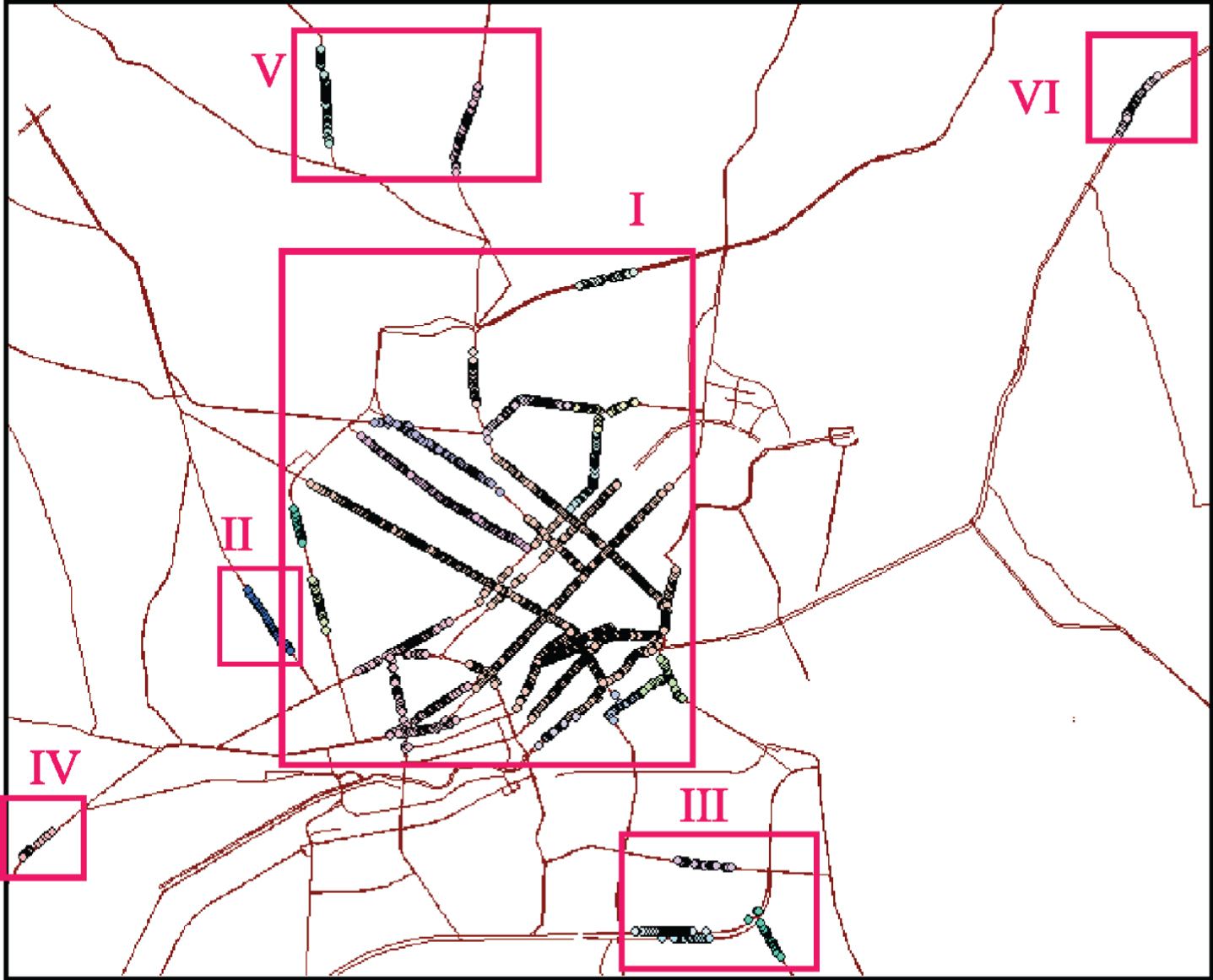
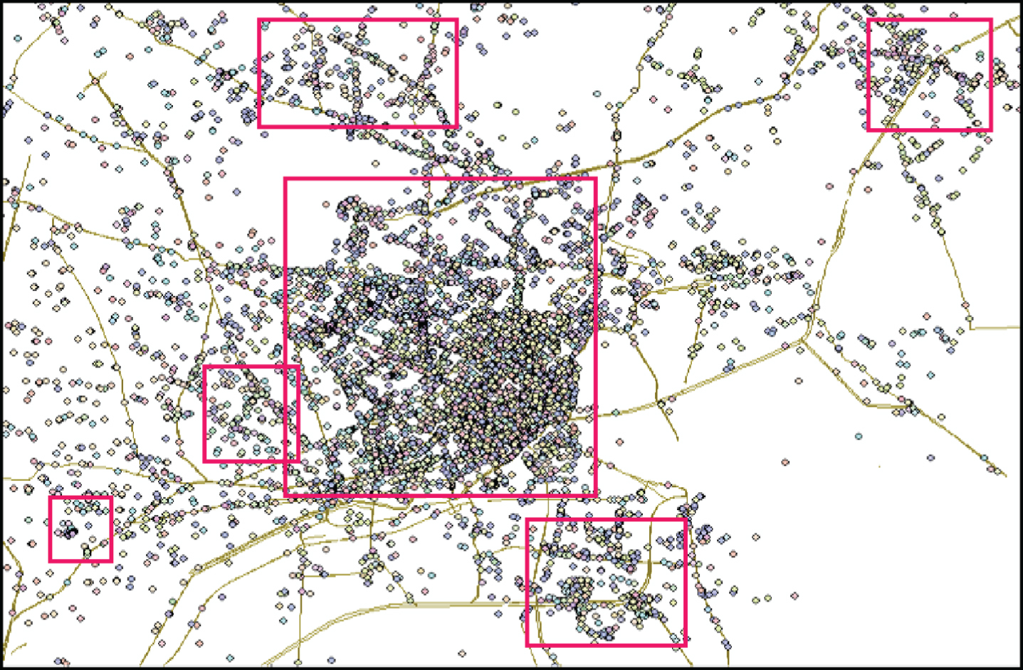
The clusters of the NS-DBSCAN algorithm (eps = 300, MinPts = 30) accurately delineated the six highly populated regions of aggregated POIs.

Fig. 10

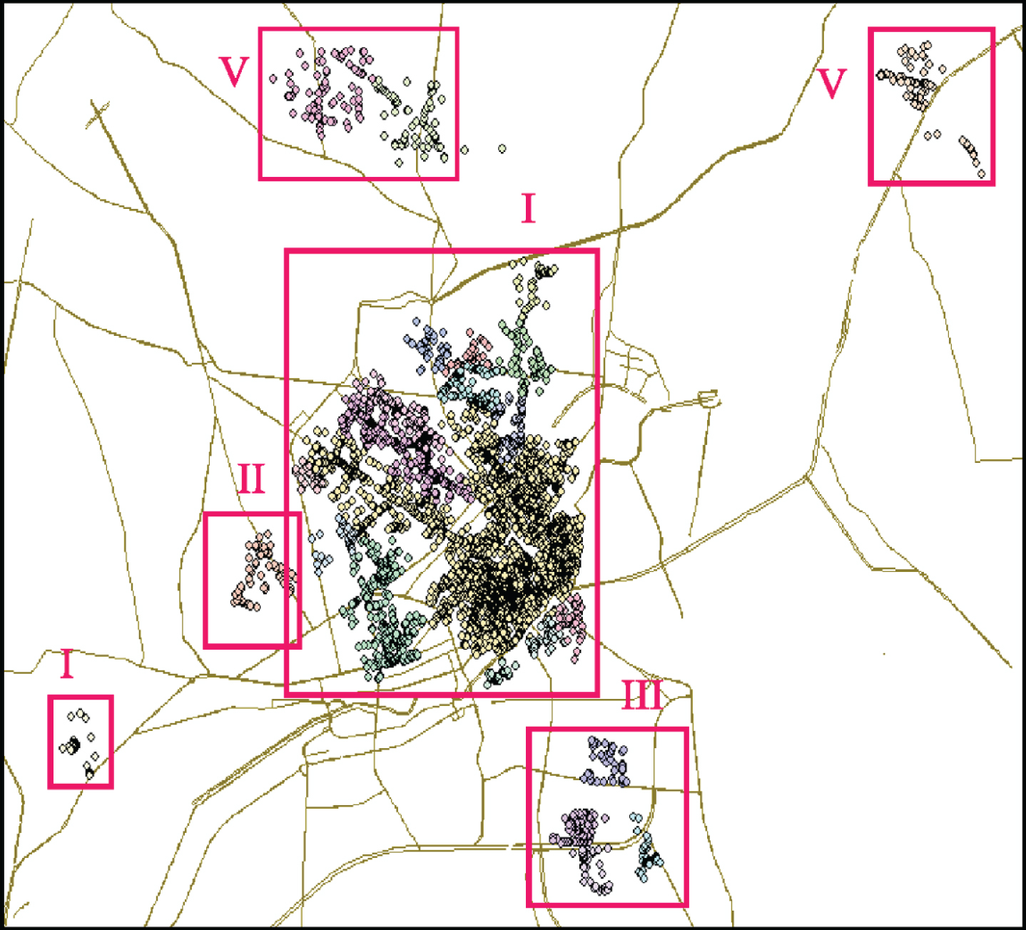
The points of interest (POIs) of Ho Chi Minh City included six aggregated regions: I, Group of Districts 1, 3, 5, 10, Phu Nhuan; II, Center of District 11; III, Center of District 7; IV, Center of District Binh Chanh; V, Area of Military Technical Officers School; VI, Area of Technical Pedagogy University.

Fig. 11

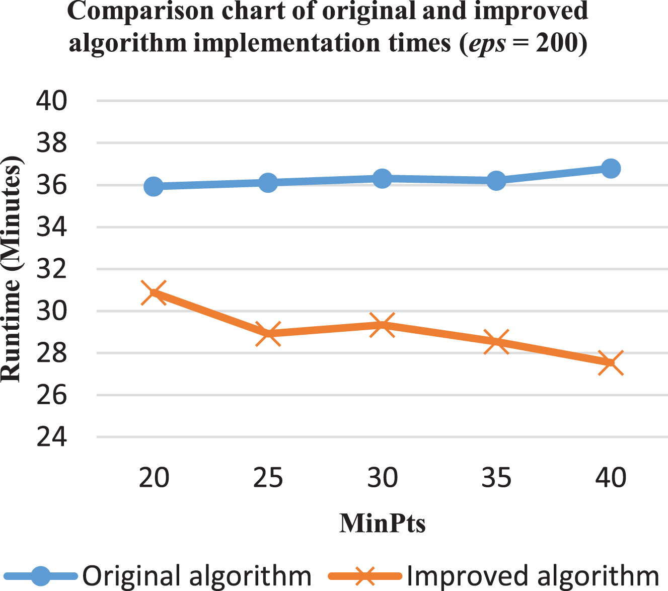
Comparison of the original and improved algorithms.

Fig. 12

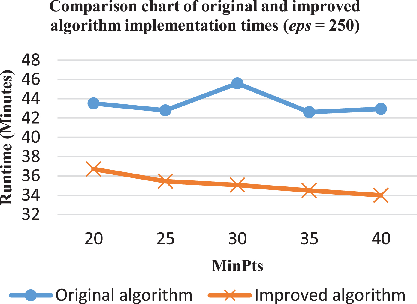
Comparison of the original and improved algorithms (eps = 250).

Fig. 13

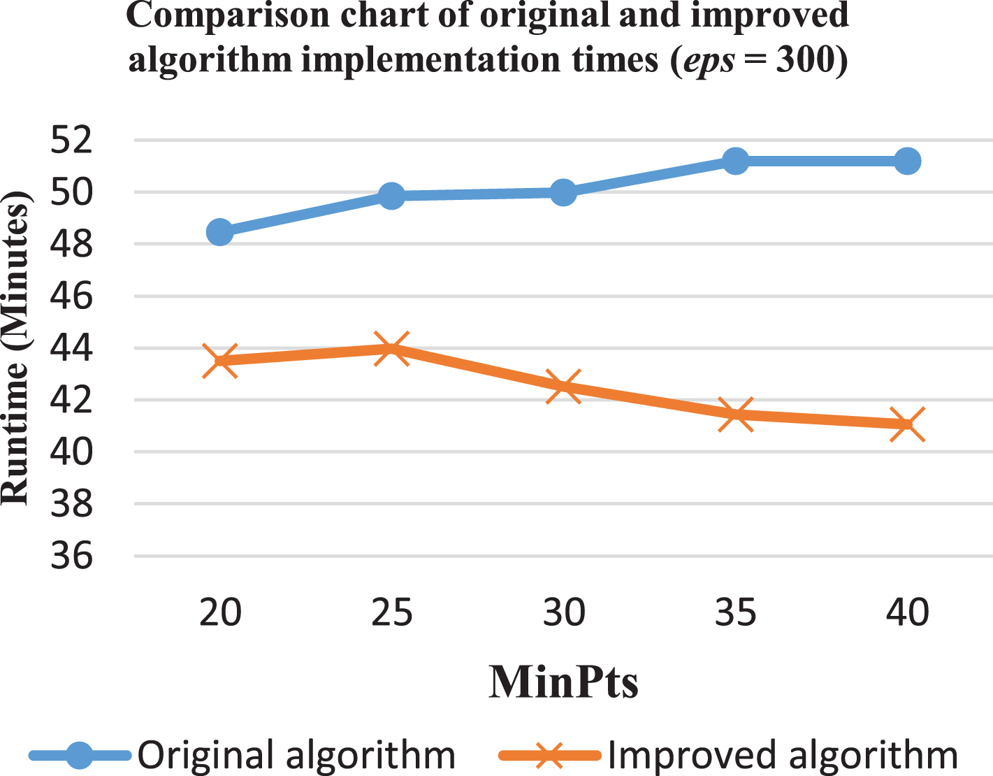
Comparison of the original and improved algorithms (eps = 300).

Fig. 14

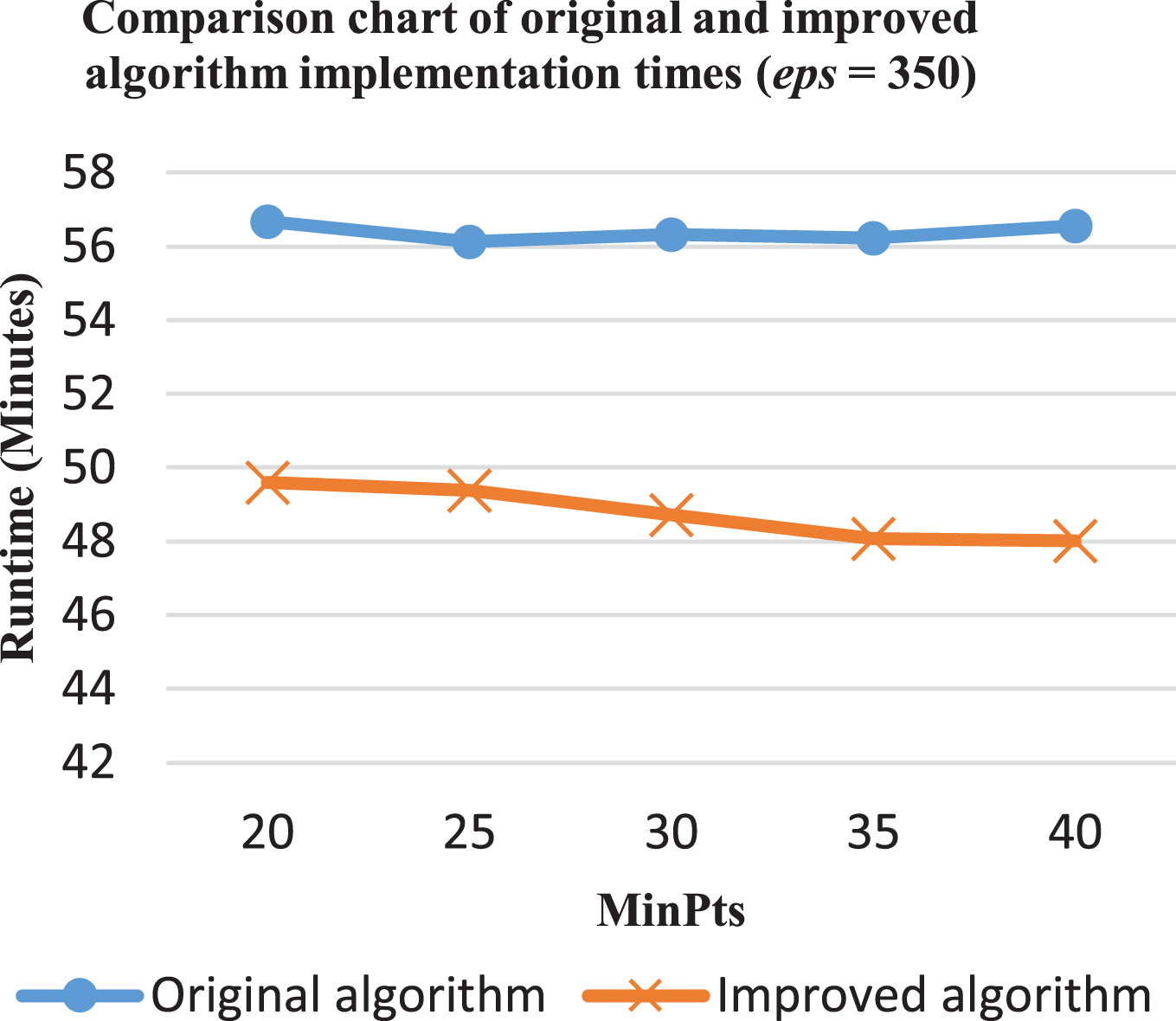
Comparison of the original and improved algorithms (eps = 350).

Fig. 15

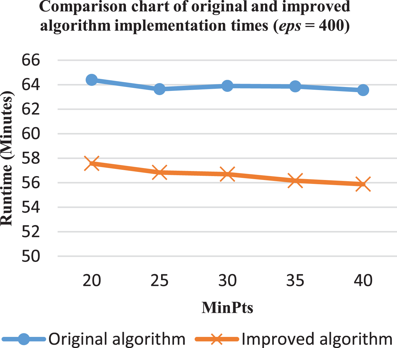
Comparison of the original and improved algorithms (eps = 400).

Figure 9 shows the clustering results of the NS-DBSCAN algorithm and proposed algorithm, and the results are expressed in real coordinates of POIs as follows (Fig. 10).

The following charts show the results of comparing the implementation time of the original algorithm with that of the improved algorithm with eps = 200, 250, 300, 350 and 400.

The chart shows a comparison of the execution time between the original and improved algorithms with a distance of 200 meters eps (Fig. 11). There is clearly a significant time difference between the original and improved algorithms. The improved algorithm needs from 14% to 25% less processing time. The lowest reduction is the case of MinPts = 20, for which the time needed fell by 14%, from 36 minutes to 31 minutes, the highest was MinPts = 40, which reduced the processing time by 25%, from 37 minutes to 28 minutes.

As when eps is 200, with eps = 250 the difference between the original and improved algorithms is significant with regard to time, ranging from 16% to 23% (Fig. 12). The most time-saving point in this case is MinPts = 30, when the processing time of the improved algorithm is 35 minutes compared to 46 minutes using the original algorithm, a fall of 23%. The remaining cases are 37 minutes compared to 44 (17% faster), 35 minutes compared to 43 (a decline of 17%), and 34 minutes compared to 43 (a fall of 19%), corresponding to threshold values of MinPts of 20, 25, 35, and 40, respectively.

In case of eps = 300, the difference in the time needed for the two algorithms ranges from 10% to 20%. The highest reduction is 20% at MinPts = 40, the lowest is 10% with MinPts = 20 (Fig. 13).

With eps = 350, the difference in processing time ranges from 12% to 15%. When MinPts = 40, it is reduced by 9 minutes, from 57 to 48. In the cases of MinPts = 20 and 25 it falls by 7 minutes, from 57 minutes to 50 and 56 minutes to 49, respectively (Fig. 14).

When eps = 400, the execution time of the algorithm falls in the range of 11% to 12% (Fig. 15).

Therefore, the experimental results show that the algorithm processing time decreases, on average, by 16%. In particular, in the situation that eps = 200 and MinPts = 20, the amoung of time for processing could fall by a crushing 25%, giving it an enormous advantage over the original algorithm. As such, the improved algorithm has been proved to be a time-saving tool to cluster data.

In addition, with data for Ha Noi, Da Nang, Can Tho, Dong Nai and a number of provinces, the results are as follows.

Ha Noi has 10,273 points and 11,683 road segments. The table shows a comparison of the execution time between the original and improved algorithms (Table 1). The highest reduction is 19% at eps = 200 and MinPts = 20.

Da Nang has 3,284 points and 8,339 road segments. The difference in the time needed for the two algorithms ranges from 0% to 15%. The highest reduction is 15% (Table 2).

Table 1

Comparison of the original and improved algorithms for Ha Noi

Eps	MinPts	Time (seconds)		Difference
		Original algorithm	Improved algorithm	(%)
200	20	3695.859	3384.595	8%
200	25	3840.874	3352.629	13%
200	30	3899.625	3318.830	15%
200	35	3916.152	3263.588	17%
200	40	3802.318	3128.325	18%
250	20	4386.433	4206.755	4%
250	25	4422.713	4175.602	6%
250	30	4475.971	4132.867	8%
250	35	4495.004	3970.790	12%
250	40	4491.186	4029.178	10%
300	20	5350.697	5088.795	5%
300	25	5379.076	5126.152	5%
300	30	5399.647	5075.637	6%
300	35	5504.518	5012.040	9%
300	40	5783.601	5037.547	13%
350	20	6335.586	5852.896	8%
350	25	6248.493	5910.224	5%
350	30	6319.992	5828.038	8%
350	35	6083.536	6181.583	-2%
350	40	6917.174	6603.903	5%
400	20	8141.048	7067.130	13%
400	25	8166.441	7164.340	12%
400	30	8140.506	7211.633	11%
400	35	8119.242	7178.907	12%
400	40	7230.045	7196.679	0%

Table 2

Comparison of the original and improved algorithms for Da Nang

Eps	MinPts	Time (seconds)		Difference
		Original algorithm	Improved algorithm	(%)
200	20	130.763	123.858	5%
200	25	129.061	116.888	9%
200	30	128.014	116.479	9%
200	35	122.432	117.293	4%
200	40	127.061	114.386	10%
250	20	159.204	152.954	4%
250	25	158.611	148.78	6%
250	30	160.471	152.911	5%
250	35	156.094	147.656	5%
250	40	154.875	151.234	2%
300	20	183.941	184.326	0%
300	25	185.019	181.753	2%
300	30	183.863	181.408	1%
300	35	186.285	182.831	2%
300	40	182.676	180.502	1%
350	20	214.725	212.396	1%
350	25	214.193	209.458	2%
350	30	213.146	209.303	2%
350	35	226.971	210.223	7%
350	40	221.789	214.585	3%
400	20	333.744	302.139	9%
400	25	305.439	292.204	4%
400	30	343.584	291.005	15%
400	35	329.696	286.315	13%
400	40	323.636	285.878	12%

Can Tho has 2,563 points and 6,277 road segments. The greatest difference in processing time is 15% (Table 3).

Table 3

Comparison of the original and improved algorithms for Can Tho

Eps	MinPts	Time (seconds)		Difference
		Original algorithm	Improved algorithm	(%)
200	20	71.273	68.476	4%
200	25	69.633	68.007	2%
200	30	69.914	68.930	1%
200	35	70.055	66.101	6%
200	40	69.632	67.133	4%
250	20	93.370	86.791	7%
250	25	91.759	88.008	4%
250	30	90.729	88.057	3%
250	35	90.734	87.464	4%
250	40	90.401	90.104	0%
300	20	114.982	110.186	4%
300	25	115.357	107.466	7%
300	30	115.761	111.870	3%
300	35	115.639	109.326	5%
300	40	113.388	110.997	2%
350	20	143.517	133.985	7%
350	25	143.281	135.875	5%
350	30	145.641	136.952	6%
350	35	144.860	136.077	6%
350	40	145.657	132.203	9%
400	20	182.473	160.971	12%
400	25	177.707	162.815	8%
400	30	181.114	163.628	10%
400	35	180.239	162.722	10%
400	40	180.207	163.347	9%

Dong Nai has 2,704 points and 6,958 road segments. The greatest difference in the time needed for the two algorithms is 15% (Table 4).

Table 4

Comparison of the original and improved algorithms for Dong Nai

Eps	MinPts	Time (seconds)		Difference
		Original algorithm	Improved algorithm	(%)
200	20	48.523	45.177	7%
200	25	50.690	45.881	9%
200	30	50.323	44.442	12%
200	35	48.849	44.255	9%
200	40	50.732	44.568	12%
250	20	59.544	53.912	9%
250	25	61.566	52.598	15%
250	30	60.157	51.709	14%
250	35	59.006	53.147	10%
250	40	59.135	54.350	8%
300	20	60.035	61.851	-3%
300	25	65.208	60.975	6%
300	30	64.084	62.679	2%
300	35	62.118	62.882	-1%
300	40	60.149	65.070	-8%
350	20	77.308	68.977	11%
350	25	68.805	69.053	0%
350	30	70.342	67.852	4%
350	35	73.706	69.570	6%
350	40	74.852	68.071	9%
400	20	85.590	79.071	8%
400	25	84.391	78.056	8%
400	30	80.690	78.055	3%
400	35	87.825	74.806	15%
400	40	84.150	75.882	10%

Provinces including Binh Thuan, Dak Lak, Dak Nong, Lam Dong, Ninh Thuan have 5,647 points and 15,694 road segments. The improved algorithm needs from 3% to 16% less processing time (Table 5).

Table 5

Comparison of the original and improved algorithms for Binh Thuan, Dak Lak, Dak Nong, Lam Dong and Ninh Thuan

Eps	MinPts	Time (seconds)		Difference
		Original algorithm	Improved algorithm	(%)
200	5	74.257	65.928	11%
200	10	74.899	63.930	15%
200	15	76.071	65.148	14%
200	20	76.181	64.320	16%
200	25	78.454	65.851	16%
250	5	83.540	76.712	8%
250	10	84.995	76.306	10%
250	15	85.804	78.916	8%
250	20	86.198	78.038	9%
250	25	84.667	75.665	11%
300	5	95.917	84.167	12%
300	10	94.137	83.759	11%
300	15	95.917	87.229	9%
300	20	94.870	88.027	7%
300	25	93.963	83.665	11%
350	5	104.419	97.682	6%
350	10	106.403	99.527	6%
350	15	102.075	99.074	3%
350	20	104.418	97.136	7%
350	25	105.278	98.589	6%
400	5	113.668	110.669	3%
400	10	117.514	112.480	4%
400	15	118.905	108.778	9%
400	20	116.081	112.638	3%
400	25	118.031	113.779	4%

Provinces including Ben Tre, Can Tho, Dong Thap, Hau Giang, Tien Giang, Vinh Long have 4,316 points and 14,173 road segments. The highest reduction is 16% at eps = 350 and MinPts = 15 (Table 6).

Table 6

Comparison of the original and improved algorithms for Ben Tre, Can Tho, Dong Thap, Hau Giang, Tien Giang and Vinh Long

Eps	MinPts	Time (seconds)		Difference
		Original algorithm	Improved algorithm	(%)
200	5	162.001	139.999	14%
200	10	145.193	139.203	4%
200	15	142.892	139.498	2%
200	20	140.630	142.672	-1%
200	25	149.424	138.608	7%
250	5	180.682	171.629	5%
250	10	186.416	173.169	7%
250	15	179.124	175.734	2%
250	20	185.826	177.885	4%
250	25	184.902	173.019	6%
300	5	225.152	216.226	4%
300	10	250.481	215.059	14%
300	15	239.144	230.622	4%
300	20	234.547	231.178	1%
300	25	227.597	219.535	4%
350	5	279.753	266.612	5%
350	10	289.530	272.688	6%
350	15	319.030	267.483	16%
350	20	316.069	267.795	15%
350	25	268.873	257.827	4%
400	5	331.411	317.448	4%
400	10	330.992	306.983	7%
400	15	335.318	308.099	8%
400	20	330.647	313.991	5%
400	25	333.224	313.381	6%

Provinces including Binh Dinh, Gia Lai, Kon Tum, Phu Yen, Quang Nam, Quang Ngai have 4,446 points and 18,665 road segments. The biggest difference in the time needed for the two algorithms is 15% (Table 7).

Table 7

Comparison of the original and improved algorithms in Binh Dinh, Gia Lai, Kon Tum, Phu Yen, Quang Nam and Quang Ngai

Eps	MinPts	Time (seconds)		Difference
		Original algorithm	Improved algorithm	(%)
200	5	379.786	368.839	3%
200	10	364.853	361.430	1%
200	15	371.932	370.354	0%
200	20	368.792	369.919	0%
200	25	368.930	376.996	–2%
250	5	534.914	523.843	2%
250	10	522.985	460.658	12%
250	15	526.310	453.418	14%
250	20	535.870	498.613	7%
250	25	526.402	474.363	10%
300	5	548.968	539.482	2%
300	10	542.559	539.559	1%
300	15	544.704	542.857	0%
300	20	633.448	560.787	11%
300	25	623.446	566.025	9%
350	5	713.586	634.973	11%
350	10	716.334	631.522	12%
350	15	729.131	620.552	15%
350	20	730.131	627.453	14%
350	25	729.028	633.747	13%
400	5	789.579	705.715	11%
400	10	763.666	735.181	4%
400	15	777.167	715.258	8%
400	20	725.190	693.453	4%
400	25	723.034	675.794	7%

Other cases also give the similar results to those presented above.

The improved algorithm produces the same clustering results as the original algorithm with the following silhouette measurements [40] in Table 8.

Table 8

Comparison of the silhouettes of the original algorithm and improved algorithm

Eps	MinPts	Cluster Number	Original Algorithm Silhouette	Improved Algorithm Silhouette
200	20	51	-0.02486	-0.02486
200	25	40	-0.01214	-0.01214
200	30	30	-0.00333	-0.00333
200	35	21	0.19976	0.19976
200	40	19	0.20985	0.20988
250	20	48	-0.07762	-0.07772
250	25	34	-0.00422	-0.00422
250	30	31	0.01146	0.01146
250	35	23	-0.03283	-0.03283
250	40	19	-0.04797	-0.04797
300	20	41	-0.00358	-0.00358
300	25	37	-0.07088	-0.07088
300	30	23	-0.00132	-0.00132
300	35	22	-0.06759	-0.06759
300	40	22	0.02430	0.02430
350	20	37	-0.12758	-0.12758
350	25	34	-0.15283	-0.15283
350	30	29	-0.10506	-0.10506
350	35	23	0.00182	0.00182
350	40	19	-0.02559	-0.02559
400	20	36	-0.08231	-0.08231
400	25	30	-0.09471	-0.09471
400	30	24	-0.11746	-0.11746
400	35	23	-0.06400	-0.06400
400	40	21	-0.08206	-0.08206

The indicators for evaluating the effectiveness of the NS-DBSCAN algorithm compared with NC_DT and hierarchical clustering algorithms [3] are shown in Table 9.

Table 9

Indicators for Evaluating the Effectiveness of Clustering Algorithms [3]

Clustering Algorithms	Parameters	Cluster Number	Silhouette	RS	DB	SB
NC_DT		37	–0.5054	0.2215	0.8167	0.0364
Algorithm	closest-pair distance	10	0.0164	0.5517	0.4878	0.0887
	farthest-pair distance	36	0.3949	0.9739	0.9251	0.0264
Heirarchical	average-pair distance	10	0.4466	0.9031	0.7822	0.0866
Algorithm	median-pair distance	23	0.3420	0.9446	0.8121	0.0393
	radius distance	16	0.4292	0.9426	0.6821	0.0518
	eps = 100, MinPts = 10	60	0.4470	0.9968	0.4047	0.0131
	eps = 100, MinPts = 15	38	0.4296	0.9978	0.5004	0.0166
	eps = 100, MinPts = 20	21	0.6740	0.9999	0.3605	0.0180
	eps = 200, MinPts = 15	38	0.2002	0.9719	0.5375	0.0095
NS-DBSCAN	eps = 200, MinPts = 20	31	0.4187	0.9913	0.4407	0.0088
Algorithm	eps = 200, MinPts = 25	28	0.4703	0.9952	0.4456	0.0113
	eps = 300, MinPts = 20	24	0.2902	0.9628	0.5473	0.0145
	eps = 300, MinPts = 25	23	0.2608	0.9666	0.5213	0.0121
	eps = 300, MinPts = 30	20	0.3220	0.9681	0.4860	0.0119
	eps = 400, MinPts = 25	14	0.3424	0.9307	0.5812	0.0262
	eps = 400, MinPts = 30	16	0.3560	0.9564	0.5610	0.0194
	eps = 400, MinPts = 35	17	0.3777	0.9625	0.5098	0.0158

6 Conclusion and future works

In this article, we have presented an efficient method, NS-DBSCAND, to help reduce processing time. In Algorithm 1 (LSPD), we determine the neighbor of the central point (cp) within an eps radius to form a set of all points within eps distance from cp by extending the line from cp to its adjacent points. The expansion to the adjacent points lasts until the expanded path is no longer shorter than the current length or it exceeds eps. As such, the expansion path will definitely not go beyond the edges whose length exceeds eps. Therefore, the first recommendation is to remove the edges whose length exceeds the eps distance when organizing data. Secondly, when generating the density ordering table, we do not include points whose density is lower than ln (10, 352) ≈ 9, according to [38]. The elimination of these points helps reduce the number of browsing points in Algorithm 3 (The original algorithm works by calculating the density for all event points and putting all vertices into the density ordering table, even those points with a density of 0). This does not affect the result because low-density points definitely do not belong to any clusters. Thirdly, some improvements in programming techniques are made to reduce computational operations and the processing time of the algorithm, as assessed in Section 3.

The most important and time-consuming operation of the NS-DBSCAN algorithm is to identify neighbors for all points, and it fares worse when processing a sequence which consists of an enormous number of points. Therefore, one future development direction is to simultaneously identify neighbors for multiple points using parallel programming techniques to reduce the algorithm’s implementation time. Distributed data processing using MapReduce is one method that may accomplish this goal.

In addition, more clustering methods will be considered for use in clustering the network space in the future works, like clustering by fast search and find of density peaks [41].

References

Wang

and Yuan

, Spatial data mining: A perspective of big data, International Journal of Data Warehousing and Mining (IJDWM) 10(4) (2014), 50–70.

Wang

and Surapunt

, “Spatial Data Mining,” in Encyclopedia of Big Data Technologies, Springer, 2019, pp. 27–32.

Wang

, Ren

, Luo

and Tian

, NS-DBSCAN: A Density-Based Clustering Algorithm in Network Space, International Journal of Geo-Information 8(5) (2019), 218.

, Luo

and Vo

, Time seriers trend analysis based K-means and support vector machine, Computing and Informatics 35(1) (2016), 111–127.

Park

H.S.

and Jun

C.H.

, A simple and fast algorithm for K-medoids clustering, Expert Systems with Applications 36(2) (2009), 3336–3341.

Zhang

, Ramakrishnan

and Livny

, BIRCH: An efficient data clustering method for very large databases, ACM SIGMOD 25(2) (1996).

Guha

, Rastogi

and Shim

, CURE: an efficient clustering algorithm for large databases, ACM SIGMOD 26(1) (2001), 35–58.

R.T.

and Han

, CLARANS: A Method for Clustering Objects for Spatial Data Mining, IEEE Transactions on Knowledge and Data Engineering 14(5) (2002), 1003–1016.

Ester

, Kriegel

H.-P.

, Sander

and Xu

, A Density-Based Algorithm for Discovering Clusters in Large Spatial Databases with Noise,” Proceedings of the Second International Conference on Knowledge Discovery and Data Mining (1996), 226–231.

10.

Ankerst

, Breunig

M.M.

, Kriegel

H.-P.

and Sander

, OPTICS: ordering points to identify the clustering structure, ACM SIGMOD 28(2) (1999).

11.

Hinneburg, Alexander, Gabriel and Hans-Henning, “DENCLUE 2.0: Fast Clustering Based on Kernel Density Estimation,” in Advances in Intelligent Data Analysis VII, Springer, 2007.

12.

Mai

, Janowicz

, Hu

and Gao

, ADCN: An anisotropic density-based clustering algorithm for discovering spatial point patterns with noise, Transaction in GIS 22(1) (2018), 348–369.

13.

Gan

, Ma

and Wu

, Data Clustering: Theory, Algorithms, and Applications, Society for Industrial and Applied Mathematics, 2007.

14.

Liu

, Huang

, Fei

, Wang

and Liang

, Constraint-based clustering by fast search and find of density peaks, Science Direct 330 (2019), 223–237.

15.

, Zhou

and Wang

, F-DPC: Fuzzy Neighborhood-Based Density Peak Algorithm, IEEE Access 8 (2020), 165963–165972.

16.

Zhao

, Chen

, Yang

, Zou

and Wang

Z. J.

, ICFS Clustering With Multiple Representatives, IEEE Transactions on Neural Networks and Learning Systems 30(3) (2019), 728–738.

17.

Fan

, Qiu

and Yuan

, Adaptive core fusion-based density peak clustering for complex data with arbitrary shapes and densities, Science Direct 107, 2020.

18.

Flores

K.G.

and Garza

S.E.

, Density peaks clustering with gap-based automatic center detection, Knowledge-Based Systems 206 (2020).

19.

Schikuta

, “Grid clustering:An efficient hierarchical clusteringmethod for very large data sets,” In 13th International Conference on Pattern Recognition, 2002.

20.

Yanchang

and Junde

, “GDILC: a grid-based density-isoline clustering algorithm,” In 2001 International Conferences on Info-Tech and Info-Net, 2002.

21.

Sheikholeslami

, Chatterjee

and Zhang

, WaveCluster: a wavelet-based clustering approach for spatial data, VLDB Journal 8 (1999), 289–304.

22.

Liu

, Deng

, Shi

and Wang

, A density-based spatial clustering algorithm considering both spatial proximity and attribute similarity, Computers & Geosciences 46 (2012), 296–309.

23.

Moon

, The Expectation-Maximization Algorithm, IEEE Signal Processing Magazine 13(6) (1996), 47–60.

24.

Kohonen

, Essentials of the self-organizing map, Neural Networks 37 (2013), 52–65.

25.

Roman

and Ivan

, Model and Principles for the Implementation of Neural-Like Structures Based on Geometric Data Transformations, International Conference on Computer Science, Engineering and Education Applications 754 (2018), 578–587.

26.

Baglietto

, Gigante

and Giudice

P.D.

, “Density-based clustering: A ‘landscape view’ of multi-channel neural data for inference and,” Plos one, 2017.

27.

Mukherjee

, Goswami

, Yang

, Tyagi

S.K.S.

, Samal

U.C.

and Mohapatra

S.K.

, “Deep neural network-based clustering technique for secure IIoT,” SpringerLink 2020.

28.

Bhattacharjee

and Mitra

, “A survey of density based clustering algorithms,” Front. Comput. Sci. 2020.

29.

Liu

, Liu

, Yu

and Ma

, “A Double-Density Clustering Method Based on “Nearest to First in” Strategy,” MDPI, 2020.

30.

Wan

and Wang

Y.-P.

, “The Comparison of Density-Based Clustering Approach among Different Machine Learning Models on Paddy Rice Image Classification of Multispectral and Hyperspectral Image Data,” Agriculture 2020.

31.

Lulli

, Dell’Amico

, Michiardi

and Ricci

, “NG-DBSCAN: Scalable Density-Based Clustering for Arbitrary Data,” ACM 2016.

32.

J.-H. C. J.-H. K. J.-H. C. Jeong-Hun Kim, “AA-DBSCAN: an approximate adaptive DBSCAN for finding clusters with varying densities,” The Journal of Supercomputing, p. 142–169, 2017.

33.

Jang

and Jiang

, “DBSCAN++: Towards fast and scalable density clustering,” in Proceedings of the 36th International Conference on Machine Learning, 2019.

34.

Jungnickel and Dieter, “Shortest Paths,” in Graphs, Networks and Algorithms. Algorithms and Computation in Mathematics, Springer, 2008, pp. 59–95.

35.

“wikipedia,” [Online]. Available: https://en.wikipedia.org/wiki/DBSCAN.

36.

Schubert

, Sander

, Ester

, Kriegel

H.-P.

and Xu

, DBSCAN Revisited, Revisited: Why and How You Should (Still) Use DBSCAN, ACM Transactions on Database Systems 42(3) (2017), 1–21.

37.

Devkota

, Miyazaki

, Witayangkurn

and Kim

S.M.

, Using Volunteered Geographic Information and Nighttime Light Remote Sensing Data to Identify Tourism Areas of Interest, Sustainability 11(17) (2019), 4718.

38.

Birant

and Kut

, ST-DBSCAN: An algorithm for clustering spatial–temporal data, Data & Knowledge Engineering 60(1) (2007), 208–221.

39.

Haklay and Mordechai , How Good is Volunteered Geographical Information? A Comparative Study of OpenStreetMap and Ordnance Survey Datasets, Environment and Planning B: Planning and Design 37(4) (2010), 682–703.

40.

Rousseeuw

P.J.

, Silhouettes: A graphical aid to the interpretation and validation of cluster analysis, Science Direct 20 (1987), 53–65.

41.

Rodriguez

and Laio

, Clustering by fast search and find of density peaks, Science 344(6191) (2014), 1492–1496.