Statement spectrum with two dimensional eigenvalues for intelligent software fault localization

Abstract

The existing Software Fault Localization Frameworks (SFLF) based on program spectrum for estimation of statement suspiciousness have the problems that the feature type of the spectrum is single and the efficiency and precision of fault localization need to be improved. To solve these problems, a framework 2DSFLF proposed in this paper and used to evaluate the effectiveness of software fault localization techniques (SFL) in two-dimensional eigenvalues takes both dynamic and static features into account to construct the two-dimensional eigenvalues statement spectrum (2DSS). Firstly the statement dependency and test case coverage are extracted by the feature extraction of 2DSFLF. Subsequently these extracted features can be used to construct the statement spectrum and data flow spectrum which can be combined into the optimized spectrum 2DSS. Finally an estimator which takes Radial Basis Function (RBF) neural network and ridge regression as fault localization model is trained by 2DSS to predict the suspiciousness of statements to be faulty. Experiments on Siemens Suit show that 2DSFLF improves the efficiency and precision of software fault localization compared with existing techniques like BPNN, PPDG, Tarantula and so fourth.

Keywords

Fault localization framework program spectrum feature extraction RBF neural network ridge regression

1 Introduction

As software continually grows in size and complexity, software faults are inevitable. These software faults are usually very subtle in tens of thousands of codes and bring down software quality. The process to ensure software quality called debugging is becoming more important. However, the process, debugging approximately accounts for about 75% of the software development costs, and it’s time-consuming and tedious [1]. Thus, to improve the software quality and reduce the costs of debugging, the research on SFL is absolutely essential.

At present, many approaches have been proposed to locate the software faults from various perspectives of program feature extraction and analysis [2, 3]. Slicing-based fault localization [4, 5] including static slicing, dynamic slicing and execution slicing abstracts a program into a reduced form by deleting irrelevant parts. Model-based fault localization [6 –8] compares the description of the correct behavior of the system model to the observed behavior. The difference between the actual model and observed behavior may lead to model components that, when assumed to deviate from their normal behavior, may explain the observed behavior. Mutation-based fault localization (MBFL) [9 –11] utilizes the number of killed mutants generated by mutating a given program element. And spectrum-based fault localization (SBFL) [12, 13] transforms test case coverage of program into program spectrum. The program spectrum can be efficiently applied to analyze program faults through machine learning techniques [14, 15], SBFL formulas [16 –18] and so on. And the efficiency of SBFL to locate faults is influenced by a number of factors [19], such as partial evaluation [20], test case suit issues [21, 22], background noise [23], coincidental correctness [24], class imbalance problem [25] and so on.

Yu et al. [26] proposed to use three program spectra including statement spectrum, control flow spectrum and data flow spectrum of program to find the location of the fault. They applied SBFL formulas like Tarantula [27], O^p [28] and CrossTab [29] which were originally used in other fields or designed by researchers based on the summary of fault localization hypotheses [30, 31], to calculate the suspiciousness of each statement in these three spectra respectively. And they took the maximum of the three as the final statement suspiciousness. However, they just separately applied these three spectra without synthetically considering statement dependency into one spectrum.

Research by Zhang et al. [32] showed the program structure inherently affects the SBFL formula and may casuse it to assign exaggerated (i.e., higher than the actual) suspicious scores or reduced suspicious scores (i.e., lower than the actual) to program entities. They proposed a new Delta4Ts model, which can significantly improve the precision of these SBFL formulas by referencing the debugging history, thereby reducing the negative effects of structural deviation. The idea of referencing prior knowledge or learning knowledge to facilitate fault localization is not novel. For example, Neelofar et al. [33] designed SBFL formula by learning parameters to drive hyperbolic functions. Sohn and Yoo [34] combined the statement scores generated by 33 SBFL formulas with the code metrics of the statement into a new feature vector, and then used genetic programming and SVM training to obtain a predictor of the statement suspiciousness.

Zhang and Li et al. [35] proposed a lightweight technique that boosts SBFL using PageRank algorithm (PRFL). PRFL uses the PageRank algorithm to recompute the statement spectrum information by differentiating tests, which has been demonstrated to outperform state-of-the-art SBFL techniques significantly. Neelofar et al. [12] found that more than 75% faulty statements were conditional statements, assignment statements and return statements on the Siemens Suit and Space Suit. Therefore, they used scripts to classify these statements in program and assigned appropriate weights to them to improve the SBFL. To improve the efficiency of SBFL, this paper also distinguishes the contribution of test cases by information quantity and applies Z-Score to calculate statement weights.

The probabilistic program dependence graph (PPDG) was proposed in [36], which facilitated probabilistic analysis and reasoning about uncertain program behavior. And the conditional probability of each node in their trained PPDG represented the likelihood to be faulty. They presented evidence indicating that PPDG could be useful for fault comprehension.

Moreover, many neural network algorithms are also applied to this field, and perform better than SBFL formulas in fault localization efficiency. Wong et al. [14] proposed a statement spectrum fault localization method using RBF neurual network. They replaced the euclidean distance in the RBF with the cosine distance to enhance the differences among different test case coverage which are eigenvectors consisting of 0 and 1, and their experimental results showed the RBF-NN was better than SBFL formulas in fault localization efficiency such as Tarantula, CrossTab, etc. Back Propagation Neural Network(BPNN) [37], a popular algorithm is regularly applied to fault localization. BPNN may lead to problems like local minima as its local search optimization strategy. Hence, Heris et al. [15] proposed a weighted BPNN of software fault localization using statement spectrum, applied the weighted method, Z-Score to assign larger initial weights to these statements covered more often by failure test cases, and decreased the search space to achieve optimal weights and improve the BPNN accuracy. And their experimental results showed the weighted BPNN improved the fault localization efficiency of BPNN. What’s more, many other learning algorithms like DNN [38] are also applied to SFL and have a satisfactory performance.

In addition to feature selection and model optimization, the refinement of the suspicion list of the model’s output results also helps to compensate for the instability of SFL caused by the complexity of the model and program. Wang et al. [39] proposed two fault triggering models called RIPR_α and RIPR_β to refine statement suspicion list. The approach can troubleshoot some higher ranked statements which are not covered by any failure test cases. Cui et al. [40] also improved the efficiency of SFL by sorting the statement suspicion list twice. First, they used SBFL to evaluate the faulty program and rank statements based on their suspiciousness, and then used MBFL to re-rank the first n statements. Li et al. [41] proposed a multi-technique fusion approach (FA) based on statement suspicion list, which merged various of randomly selected fault localization techniques to minimize the difference between the numbers of statements that need to be examined to find the bug respectively in the worst and best assumptions, further improve the effectiveness of fault localization.

Different types of program spectrum [9, 13] respectively represent diverse program dynamic features, which not only show the normal features of the program but also expose the abnormal features of the program in different aspects. However, most of methods just make use of statement spectrum which records execution states of statements and execution results under test cases to train fault localization model. The statement spectrum [12] only contains partial dynamic features, and applies two eigenvalues 1 and 0 to represent executed and unexecuted states of statements, respectively. Although the test case suits like Siemens, Space and etc have lots of test cases, a large number of statements still have the same execution states under all test cases. Thus, many statements always keep the same eigenvalues under all test cases in statement spectrum, and the fault localization model trained by the statement spectrum will generate the same suspiciousness for these statements and have an unstable fault localization efficiency. What’s more, the statements’ eigenvalues in statement spectrum are just about the statement execution states, which may not be enough to improve the fault localization efficiency or precision further. In order to overcome these problems, this paper proposes a fault localization framework (2DSFLF) and uses the 2D statement spectrum (2DSS) optimized by statement spectrum and data flow spectrum [42, 43] to train the 2DSFLF. The 2D and SFLF stand for the optimization statement spectrum with two-dimensional eigenvalues (2DSS) and software fault localization framework respectively.

In the Experimental Results section, we demonstrate the effectiveness of 2DSFLF around three research questions, namely the effectiveness of 2DSS, the effectiveness of the kernel function in our fault localization model, and the fault localization efficiency and precision of 2DSFLF. Major contributions of this paper are summarized as follows: (1) Constructing the software fault localization framework (2DSFLF) which takes both the statement execution states and statement dependency into account to locate the program faults. (2) Proposing the 2DSS which combines the statement spectrum with the data flow spectrum and refines the features of statements. (3) Proposing the algorithm of 2DSFLF construction used to generate the matrix of 2DSS and the 2DSFLF fault localization model. (4) Experimenting on Siemens Suit to prove that the 2DSFLF improves the efficiency and precision of fault localization.

The rest of this paper is organized as follows. Section 2 mentions briefly background of fault localization which contributes to understanding this paper. Section 3 analyzes the benefits of 2D statement spectrum and presents the overall process to locate the faults in our approach. Section 4 explains the proposed fault localization framework 2DSFLF and the algorithm of 2DSFLF construction. Section 5 reports the results of our experiments by comparing the 2DSFLF with other SFLF in fault localization efficiency and precision, followed by discussions on potential threats to the validity of our approach in section 6. Finally, we conclude this paper and discuss future works in section 7.

2 Background

This section gives a brief introduction about the weighted strategies, the relevant learning algorithms used in 2DSFLF and the program spectrum.

2.1 Information quantity and Z-Score

Information quantity I (t) in Eq. (1) is a weighted strategy to measure the importance of events, and the t and P (t) represent an event and its occurence probability respectively. Usually the smaller P (t) is, the larger I (t) is, so these events that occur rarely are very important and have larger I (t). For fault localization, t and P (t) represent the test cases and their occurence probability. Generally the number of failure test cases whose actual program output are different from the expected results are far fewer than the number of success test cases whose actual program output are the same as the expected results, and these failure test cases contribute more to fault localization than success test cases. The weighted strategy of information quantity is useful for measuring the contribution of success and failure test cases to fault localization, and will assign greater weights to failure test cases than success test cases, as the occurence probability of failure test cases is smaller than the occurence probability of success test cases.

One of the fault localization hypotheses summaried by Wong et al. [31]: the suspiciousness of each statement is inversely proportional to the number of each statement covered by success test cases, and the suspiciousness of each statement is proportional to the number of each statement covered by failure test cases. The data standardization processing method, Z-Score shown in Eq. (2) is adopted to respectively evaluate statements’ ZF-Score in Eq. (3) for failure test cases and statements’ ZS-Score in Eq. (4) for success test cases according to data flow spectrum. And the ZF-Score and ZS-Score measure statement coverage in data flow spectrum by failure and success test cases separately. For ZF-Score, n_f, μ_f and σ_f are the number of target statement covered by failure test cases, the average and variance of the number of statements in program covered by failure test cases. In the similar way, the n_s, μ_s and σ_s for ZS-Score are the corresponding values when statements are covered by success test cases. The statements with greater ZF-Score and smaller ZS-Score are generally covered more by failure test cases and less by success test cases, so they’ll have a larger suspiciousness according to the fault localization hypothesis. $I (t) = \log (\frac{1}{p (t)})$ (1) $Z - Score = \frac{n - μ}{σ}$ (2) $ZF - Score = \frac{n_{f} - μ_{f}}{σ_{f}}$ (3) $ZS - Score = \frac{n_{s} - μ_{s}}{σ_{s}}$ (4)

2.2 Ridge regression and neural network

As compared to linear regression, ridge regression typically is used to deal with the case where the number of features is more than sample size, and add a penalty factor λ in Eq. (5) to linear regression estimate to get a better estimate. As λ approaches to 0, the estimator $W$ is closer to the unbiased estimation of the least square method. Instead, the estimator $W$ will deviate from unbiased estimation and tend to 0 with the increase of λ. Thus, the ridge regression which adds the penalty factor λ to the matrix ${XX}^{T}$ is a compromise between stability and unbiasedness, and adapts to most regression analysis problems through the adjustment of penalty factor λ. $W = ({XX}^{T} + λ E)^{- 1} X^{T} Y$ (5)

As shown in Figure 1, the structure of neural network [14 , 38] consists of input layer, hidden layers, output layer and connection weights between adjacent layers. What’s more, each neuron in the hidden layers summarizes the input data and maps them to a higher dimensional space through the activation function, and then outputs them to the neurons of next layer. The activation function of hidden layers can transform the original complex nonlinear relationship problem into a simple linear relationship problem in high-dimensional space, and the neural network applied in our framework takes the Gaussian Radial Basis Function as the activation function. Neural networks have evolved from the early feedforward neural networks to feedback neural networks, and then to the current popular deep neural networks, and a variety of algorithms have been derived to flexibly solve many scientific and engineering problems including SFL.

Fig. 1

The neural network model for falut localization.

Table 1

The detailed information of program ‘modify_mid’

	Program statements	2D statement spectrum												Results of 2DSFLF
#	void modify_mid(){	T ₁		T ₂		T ₃		T ₄		T ₅		T ₆		2D statement spectrum		statement spectrum

#	int x, y, z, m;	D ₁	D ₂	D ₁	D ₂	D ₁	D ₂	D ₁	D ₂	D ₁	D ₂	D ₁	D ₂	susp.	rank	susp.	rank
S₁	read(x, y, z);	1	0.4	1	0.4	1	0.4	1	0.4	1	0.4	1	0.4	0.7803	2	0.1378	1
S₂	x = x - 1;	1	0.08	1	0.001	1	0.001	1	0.8	1	0.001	1	0.001	0.5063	4	0.1378	1
S₃	y = y - 1;	1	0.4	1	0.04	1	0.04	1	0.04	1	0.04	1	0.04	0.7803	2	0.1378	1
S₄	m = z -1;	1	0.4	1	-0.02	1	-0.02	1	0.4	1	-0.02	1	-0.02	0.7874	1	0.1378	1
S₅	if (y <z){	1	-0.23	1	-0.001	1	-0.001	1	-0.23	1	-0.001	1	-0.001	0.3207	6	0.1378	1
S₆	if (x <y)	0	-0.23	0	-0.001	0	-0.001	1	-0.23	1	-0.001	1	-0.001	0.2094	9	0.0899	9
S₇	m = y;	0	-0.23	0	-0.001	0	-0.001	0	-0.23	0	-0.001	1	-0.001	0.0762	13	0.0385	13
S₈	else if (x <z)	0	-0.23	0	-0.001	0	-0.001	1	-0.23	1	-0.001	0	-0.001	0.2314	7	0.0937	7
S₉	m = x;}	0	-0.23	0	-0.001	0	-0.001	0	-0.23	1	-0.001	0	-0.001	0.0859	11	0.0417	11
S₁₀	else{ if (x >y)	1	-0.23	1	-0.001	1	-0.001	0	-0.23	0	-0.001	0	-0.001	0.2094	9	0.0899	9
S₁₁	m = y;	0	-0.23	0	-0.001	1	-0.001	0	-0.23	0	-0.001	0	-0.001	0.0762	13	0.0385	13
S₁₂	else if(x >z);	1	-0.23	1	-0.001	0	-0.001	0	-0.23	0	-0.001	0	-0.001	0.2314	7	0.0937	7
S₁₃	m = x;	0	-0.23	1	-0.001	0	-0.001	0	-0.23	0	-0.001	0	-0.001	0.0859	11	0.0417	11
S₁₄s	print(m);}	1	0	1	0	1	0	1	0	1	0	1	0	0.4517	5	0.1378	1
Test Case Results: $(S_{4}^{*}^{'} F m = z)$		1		0		0		1		0		0

2.3 Program spectrum

The program spectrum [2] generally consists of the coverage of all program entities and the test case execution results. The program entities can be a predicate expression, a statement, a block, a function, a class and etc. And the test case results appertain to the program actual output and expected output when the program is run through test cases. The program entity of statement spectrum and 2D statement spectrum is a statement, and the program entity of data flow spectrum [42] is a dependency between two statements. In general, the number of program entities n and the minimum number of test cases m that can exactly cover all executable paths of a program form a basic spectrum matrix with the size of m * n.

3 Motivation

In order to facilitate the comprehension of 2DSFLF, three program spectra statement spectrum, data flow spectrum and 2DSS are constructed and the overall process to locate the faults using 2DSFLF is presented briefly by a small instance in this section. More details are described in next section.

3.1 Empirical study

Table 1 shows the detailed information about the program ‘modify_mid’, which are the program statement, 2D statement spectrum and the results of 2DSFLF. Each row of the program statement is an executable statement labeled S_n. The 2DSS is constituted by coverage of six different test cases, and the coverage of each test case is made up of fourteen executable statements’ eigenvalues. The eigenvalues of D₁ and D₂ are the execution states taken from statement spectrum and the statement Z-Score evaluated by data flow spectrum. The different test cases refer to these test cases which can lead to different program coverage. The last row is the test case execution results, the test cases T₁ and T₄ are failure test cases whose execution results are labeled 1, and others are success test cases whose execution results are labeled 0. And the faulty statement is S₄ which is supposed to be the statement $S_{4}^{*}$ . And the purpose of SFL is to efficiently locate the faulty statement S₄.

3.1.1 Statement spectrum

Statement spectrum whose proagram entities are executable statements distinguishes statement execution states in different test cases. As shown in Table 1, the columns of D₁ represent the execution states of all the executable statements in program ‘modify_mid’,

Table 2
The data flow spectrum and Z-Score of program ‘modify_mid’

Stat. S1 S1 S2 S2 S2 S3 S3 S3 S4 S7 S9 S11 S13

S2 S8 S6 S8 S9 S5 S6 S7 S14 S14 S14 S14 S14

T1 1 0 0 0 0 1 0 0 1 0 0 0 0

T2 1 0 0 0 0 1 0 0 0 0 0 0 1

T3 1 0 0 0 0 1 0 0 0 0 0 1 0

T4 1 1 1 1 0 1 1 0 1 0 0 0 0

T5 1 1 1 1 1 1 1 0 0 0 1 0 0

T6 1 0 1 0 0 1 1 1 0 1 0 0 0

ZF. 0.4 0.08 0.08 0.08 -0.23 0.4 0.08 -0.23 0.4 -0.23 -0.23 -0.23 -0.23

ZS. 0.04 -0.001 0.001 -0.001 -0.001 0.04 0.001 -0.001 -0.02 -0.001 -0.001 -0.001 -0.001

Stat.	S1	S1	S2	S2	S2	S3	S3	S3	S4	S7	S9	S11	S13
T1	1	0	0	0	0	1	0	0	1	0	0	0	0
T2	1	0	0	0	0	1	0	0	0	0	0	0	1
T3	1	0	0	0	0	1	0	0	0	0	0	1	0
T4	1	1	1	1	0	1	1	0	1	0	0	0	0
T5	1	1	1	1	1	1	1	0	0	0	1	0	0
T6	1	0	1	0	0	1	1	1	0	1	0	0	0
ZF.	0.4	0.08	0.08	0.08	-0.23	0.4	0.08	-0.23	0.4	-0.23	-0.23	-0.23	-0.23
ZS.	0.04	-0.001	0.001	-0.001	-0.001	0.04	0.001	-0.001	-0.02	-0.001	-0.001	-0.001	-0.001

and the eigenvalues 1 and 0 stand for executed and unexecuted states of statements respectively. Hence, the statement spectrum for program ‘modify_mid’ is composed of the eigenvalues of D₁ for six different test cases. Moreover, if only the statement eigenvalues under statement spectrum are considered, many statements such as (S₁, S₂, S₃, S₄, S₅, S₁₄) will always maintain the same eigenvalues in all test cases. This whill adversely affect the efficiency of fault localization.

3.1.2 Data flow spectrum

Table 2 shows the data flow spectrum and Z-Score of program ‘modify_mid’. The Stat. of the first row is the statements with the data dependence, and the following statements rely on the above statements. For instance, the statements of the first column S₁ and S₂, the following statement S₂ defined as an independent statement relies on the above statement S₁ defined as a dependent statement. The rows of test cases (T₁, T₂, T₃, T₄, T₅, T₆) are the coverage about the dependent statements. And ZF. and ZS. which have been adjusted in proportion to fit our framework presented in section 4.2 are the ZF-Score and ZS-Score for dependent statements evaluated by coverage in data flow spectrum using Eq. (2). For example, the ZF-Score of 0.4 and ZS-Score of 0.04 are for the dependent statement S₁ rather than S₂ in the first column. In order to extract the statement dependencies which are the program entities of data flow spectrum, the data dependence definition of statements to convert the variable dependencies and function calls to statement dependencies are defined as follows: For instance, the statement S_m : char c = e, ‘c’ is declared as a character variable and ‘e’ is an expression.

(1) All the statements referencing this variable ‘c’ and executing after S_m rely on the S_m.

(2) If the expression ‘e’ contains a variable ‘v’, S_m relies on these statements which define or transform the variable ‘v’ and execute before S_m.

(3) If the expression ‘e’ includes a function call ‘f’, S_m relies on all the return statements of function ‘f’. But if function ‘f’ doesn’t has return statements, there is no data dependence between S_m and function ‘f’.

(4) If S_m is declared in function ‘f’, furthermore the variable ‘v’ in expression ‘e’ relies on the formal parameters of function ‘f’, S_m relies on all the statements calling function ‘f’.

3.1.3 2D statement spectrum

In Table 1, the 2D statement spectrum(2DSS) proposed in this paper has the same program entities as the statement spectrum. The difference between 2DSS and statement spectrum is that the eigenvalues of program entities are of two dimensions. The first one is the execution states of statements which are the same as the eigenvalues of the statement spectrum, and the second one is the Z-Score of each statement. As shown in Table 2, each statement has two Z-Score values, ZS-Score and ZF-Score. And the second eigenvalues are the ZS-Score for statements in success test cases and ZF-Score for statements in failure test cases. The independent statements cannot be evaluated for Z-Score since the Z-Score is evaluated by coverage in data flow spectrum which just contains the coverage of dependent statements. Thus, for these independent statements in 2DSS, their second eigenvalues are set to zero. What’s more, the predicate statements like ‘if’ and ‘case’ statements are essential for a program, which determine the next execution statement and lead to different coverage of program, but these statements are usually not dependent statements. To enhance fault detection for these predicate statements, their Z-Score are not set to zero but the maximum of its own Z-Score and their next executable statements’ Z-Score. In short, the benefits of 2DSS is that two-dimensional eigenvalues refine the features of all the statements in comparison with statement spectrum or data flow spectrum, and 2DSS can express the features of all the executable statements.

3.2 The overall process of 2DSFLF to locate faults

The overall process of 2DSFLF to locate faults is summarized as follows:

Data preprocessing: Before training the 2DSFLF, the statement spectrum and Z-Score of statements which are used to construct the 2DSS need to be obtained. At first, the coverage and execution results of program under test cases can be collected by running all the test cases on the piling program. Some compile tools can easily pile into program, like the GUN Compiler Collection (GCC), Another Tool for Language Recognition Four (ANTLR4), etc. And the statement spectrum can be built with the coverage and execution results. Subsequently, we extract the variable dependencies, function calls and predicate statement nodes from source program by ANTLR4, and convert the variable dependencies and function calls into statement dependencies according to the data dependence definition of statements. Next, the data flow spectrum can be built with the statement dependencies and statement spectrum. At last, the Z-Score of each statement in data flow spectrum is calculated by Eq. (2).

The construction of 2DSS: According to the ZF-Score and ZS-Score of statements, statement spectrum, test case results and predicate statement nodes, the 2DSS shown in Table 1 can be generated by our algorithm presented in section 4.2. The $X$ one of the algorithm output is the 2DSS matrix with the size of m * 2n. The m is the number of different test cases, and the n is the number of executable statements. As the eigenvalues for executable statements in each test case are of two dimensions, the number of eigenvalues for each test case is twice as many as the number of executable statements.

The construction of fault localization model: Our fault localization model is a three-layer neural network, the input layer, the output layer and the hidden layer with RBF neurons. What’s more, the weights between the hidden layer and output layer are evaluated by ridge regression. And a statement suspiciousness predictor of 2DSFLF can be generated after the model is trained by 2DSS. More details are presented in section 4.1.

The fault localization report generation: At first the 2D virtual spectrum [14] of program presented in section 4.1.2 is construted and input into the statement suspiciousness predictor to generate the suspiciousness of statements. At last these statements can be sorted in descending order of statement suspiciousness, as shown in Table 1 of the results of 2DSFLF. In addition, the fault localization reports about Exam-Score and Top-N presented in section 5.2 are generated to evaluate the efficiency and precision of 2DSFLF.

Fig. 2

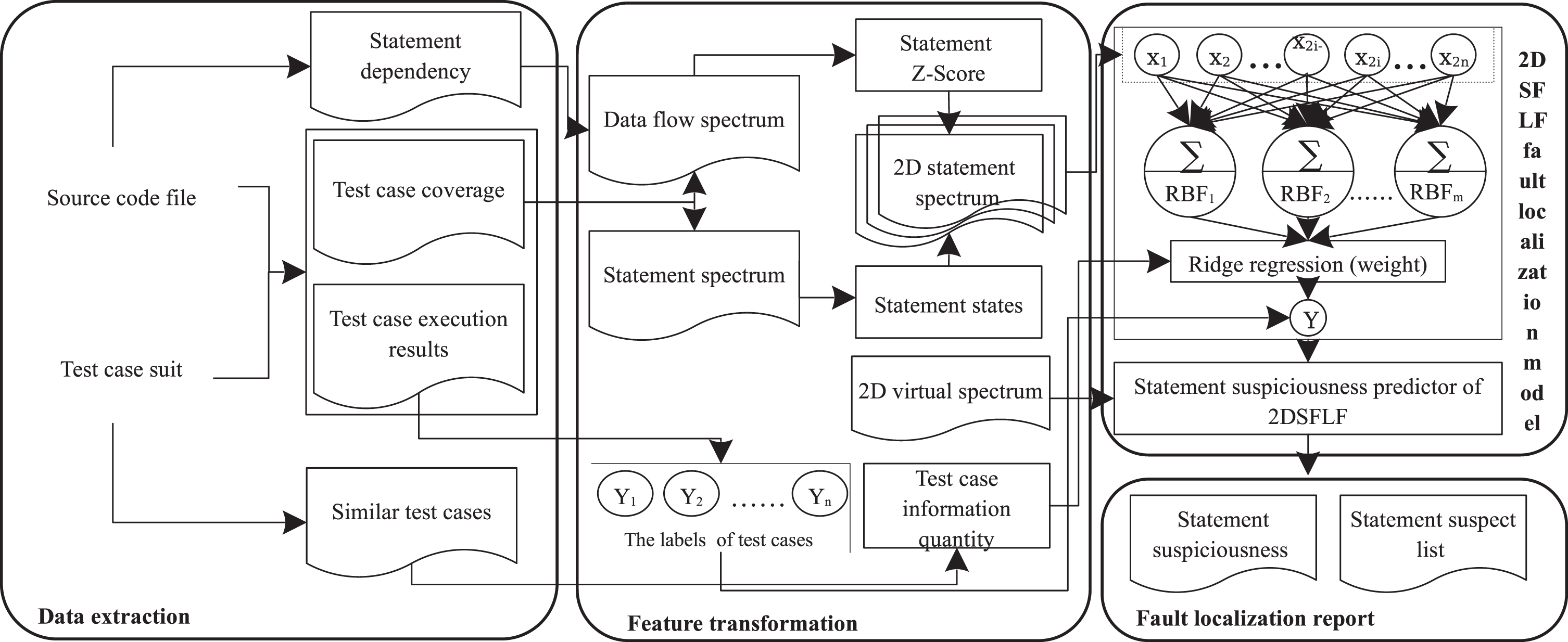
The fault localization framework of 2DSFLF.

3.3 Empirical analysis

The framework 2DSFLF is experimented on program ‘modify_mid’. The results of 2DSFLF in Table 1 are generated by the 2DSFLF when the fault localization model in 2DSFLF is trained by the 2DSS and statement spectrum respectively. The overall process of 2DSFLF to locate faults is introduced in previous section, and the construction of fault localization model and 2DSS are presented in section 4 in detail.

As shown in Table 1, the results of 2DSFLF are about the suspiciousness and ranking of each statement for two kinds of spectrum generated by 2DSFLF. The results show that the statement S₄ has the greatest suspiciousness, which means the S₄ has the maximum probability to be the faulty statement when using 2DSS to train our fault localization model. Our strategy can locate the fault with only one statement being examined, as the statement S₄ is indeed the faulty statement. When we use statement spectrum to train the same model, the results show that the statement S₄ also has the greatest suspiciousness. However, there are five other statements with the same suspiciousness as S₄, and one to six statements need to be examined to locate the faulty statement S₄. Thus, the 2DSS contributes to improving the efficiency of fault localization in comparison to statement spectrum.

4 Proposed framework

In this section, the fault localization framework 2DSFLF and the algorithm of 2DSFLF construction are presented in detail.

4.1 Framework of 2DSFLF

As shown in Figure 2, the framework, 2DSFLF is divided into four parts. The data extraction is responsible for extracting available data from the target program and test case suit. The feature transformation can convert the available data into specification data which can be directly used to train the 2DSFLF fault localization model. The remainder two parts are about the composition of the algorithm model and fault localization report respectively.

4.1.1 Data extraction

In the component of data extraction, the source code file and test case suit are taken from Siemens Suit. The test case coverage and test case execution results can be gathered by running the test case suit on the source code file. The test case coverage mark the execution states of executable statements for each test case, and the test case execution results are represented by eigenvalues 0 and 1. The eigenvalue 0 indicates that the actual output of the program is the same as the expected output, and the eigenvalue 1 indicates that the actual output is different from the expected output. Meanwhile, the statement dependency and similar test cases are extracted from source code file and test case coverage separately. The statement dependency is the program entity of data flow spectrum, such as these statements in Table 2. The six test cases in Table 1 whose coverage (the eigenvalues of D₁) differ from each other are different test cases, so the similar test cases refer to the test cases with the same coverage.

4.1.2 Feature transformation

In this component, the 2D statement spectrum(2DSS) is combined with statement states and Z-Score which are extracted from the statement spectrum and data flow spectrum respectively, and the 2D virtual spectrum can be applied as test data to generate suspiciousness of statements. The 2D virtual spectrum which consists of virtual test cases in our approach is also two-dimensional eigenvalues for each statement. In the actual operation, the coverage of each test case need to be transformed into a one-dimensional vector both in 2DSS and 2D virtual spectrum. For instance, Figure 3 shows the transformed one-dimensional vectors for the test case T₁ of 2DSS in Table1 and the virtual test case V₁, and the odd and even bits of the vectors are the first and second dimensional eigenvalues of statements respectively. The V₁ whose eigenvalues are 1 only for statement S₁ and 0 for other statements is applied to input into the statement suspiciousness predictor to generate the suspiciousness of S₁. Therefore, the V_i whose eigenvalues should be 1 only for statement S_i and 0 for other statements is used to generate the suspiciousness of S_i and the number of virtual test cases is the same as the number of statements in 2DSS.

Fig. 3

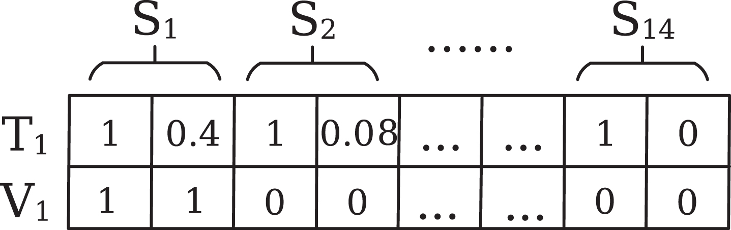
The transformed one-dimensional vector of T₁ and V₁ for program ‘modify_mid’.

The vector (Y₁, Y₂, . . . , Y_n) corresponds to the labels of test cases (T₁, T₂, . . . , T_n) in 2DSS. The information quantity $I (t)$ for test cases in 2DSS can be evaluated according to their number of similar test cases. And the information quantity $I (t)$ is calculated as follow: we still take the program ‘modify_mid’ in Table 1 as an example and assume that each test case in 2DSS only has one similar test case. Firstly count the number of similar test cases for each test case, subsequently calculate their occurence probability p (t) which are all 1/6 and the ratio of success test cases to failure test cases Ratio which is 2, lastly evaluate the $I (t)$ which is (1.56, 0.78, 0.78, 1.56, 0.78, 0.78) for (T₁, T₂, T₃, T₄, T₅, T₆) by Eq. (1). As the failure test cases contribute more to fault localization than success test cases do, their $I (t)$ are multiplied by the Ratio when the $I (t)$ for failure test cases are less than the product between the maximum $I (t)$ for success test cases and the Ratio.

4.1.3 2DSFLF fault localization model

For the upper rectangle of this component, our fault localization model is a neural network with three layers using 2DSS as training data. In the first layer, this layer is input layer whose input data is the 2DSS matrix $X$ , the input neurons correspond to the statements which have two-dimensional eigenvalues in 2DSS. Hence there are twice as many neurons as the statements in 2DSS, and the input neurons of x_2i-1 and x_2i are the first and second dimensional eigenvalues of the i_th statement respectively.

Multiple neurons with the Gaussian Radial Basis as activation function make up the second layer. Each neuron summarizes the input data from previous layer, and then ouput the processed data which has been mapped to a new dimensional space by the activation function RBF. As shown in Eq. (6) of RBF, $X_{iitsc}$ and $U_{jitsc}$ are respectively the coverage of the i_th and j_th test cases in 2DSS, and $U_{jitsc}$ is also the kernel vector for j_th neuron, the σ₀ can be calculated by Eq. (7), and the number of neurons in this layer n is the same as the number of test cases in 2DSS. For instance, the program ‘modify_mid’ has six different test cases in 2DSS, so the number of neurons n is six, and the coverage of six test cases are the kernel vectors for neurons. In addition, $| | X_{i} - U_{j} | |$ is the euclidean distance between $X_{iitsc}$ and $U_{jitsc}$ . Therefore, the second layer converts the first layer output to the matrix $R (X)$ shown in Figure 4, the R_m and T_n are the m_th neuron in this layer and the n_th test case in 2DSS respectively, and R_mn is the value to which the transformed vector of T_n is mapped by the neuron R_m.

Fig. 4

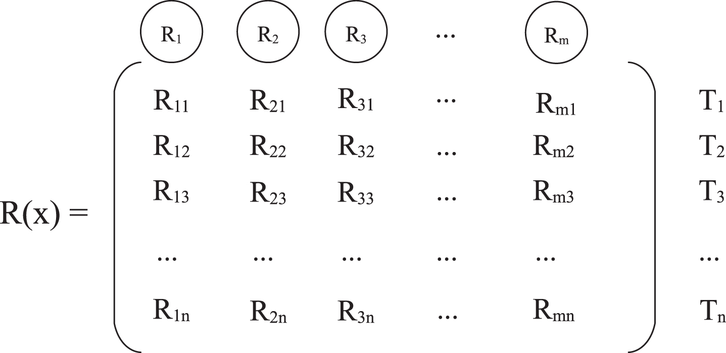
The output matrix $R (X)$ in the second layer of 2DSFLF.

In the last layer, the $Y$ is the test cases’ execution results (Y₁, Y₂, . . . , Y_n) in 2DSS. The whole neural network model is to fit the relation between $X$ and $Y$ . And the ridge regression is to further fit the relation between the $R (X)$ and $Y$ , so the weight $W$ from neurons of second layer to this layers can be calculated by Eq. (8). The $I (t)$ and $Y$ in this equation are respectively the information quantity and execution results of test cases in 2DSS, and λ is set to -0.3 in our experiments.

After the fault localization model is trained by 2DSS, a statement suspiciousness predictor of 2DSFLF for source program can be obtained. The predictor can generate the suspiciousness of corresponding statements when the 2D virtual spectrum is input into the predictor. $R_{ji} (X_{i}) = \exp (\frac{| | X_{i} - U_{j} | |^{2}}{- 2 σ_{0}^{2}}), 1 < = i, j < = n .$ (6) $σ_{0} = \max (| | X_{i} - U_{j} | |^{2}), 1 < = i, j < = n .$ (7) $W = (R (X) I (t) R (X)^{T} + λ E)^{- 1} R (X)^{T} I (t) Y$ (8)

4.1.4 Fault localization report

For the last component of the fault localization report, the statement suspiciousness is generated by the statement suspiciousness predictor and the statement suspect list consists of the statements which are sorted by their suspiciousness from large to small, so the top statements in this list are more likely to be faulty statements.

4.2 Algorithm of 2DSFLF

The Algorithm 1 gives the process of the construction of 2DSS and 2DSFLF fault localization model. For the input of the algorithm, SP is a statement spectrum matrix with the size of m * n. ZF and ZS evaluated by data flow spectrum using Eq. (2) are ZF-Score and ZS-Score for each statement. $Y$ is test case execution results for statement spectrum and PN represents all predicate statement nodes whose results (true or false) determine the next branch of program to execute. And the output of the algorithm is the matrix $X$ of 2DSS, the weight $W$ and the RBF kernel functions (R₁,R₂,...,R_m) of the 2DSFLF fault localization model in Figure 2 respectively.

Algorithm 1
2DSFLF construction algorithm

Input:SP: statement spectrum; ZF: ZF-Score; ZS:

      ZS-Score; $Y$ : test case results; PN: predicate statement

      nodes;

Output: $X$ : 2D statement spectrum; $W$ : the weight

      of third layer; (R₁,R₂,...,R_m): the kernel functions

      for second layer;

  1:  m, n ← get the size of SP

  2:   $X$ ← initialize a matrix of m * 2n

  3:maxZF, maxZS ← get the maximum from ZF and ZS

  4:ratioZF ← (0.4/maxZFAll)

  5:ratioZS ← (0.04/maxZSAll)

  6:repeat  j = 0

  7:repeat  i = 0

  8: $X$ ← SP [m, i]

  9:if $Y [j]$ is failure test case:

10:   $X [j, 2 i + 1]$ ← ZF [i] * ratioZF

11:  if $Y [j]$ is success test case:

12:   $X [j, 2 i + 1]$ ← ZF [i] * ratioZS

13:        until  i++; i > = n

14:  until:j++; j > = m

15:   repeat i = 0

16:  (curt,left,right) ← locations(PN [i])

17:  maxZF, maxZS ← maximum(ZF [curt],

      ZF [left], ZF [right]), maximum(ZS [curt],

      ZS [left], ZS [right])

18:   repeat j = 0

19:   if $Y [j]$ is failure test case:

20:   $X [j, 2 curt + 1]$ ← maxZF * ratioZF

21:  if $Y [j]$ is success test case:

22:   $X [j, 2 curt + 1]$ ← maxZS * ratioZS

23:      untilj++; j > = m

24:  untili++; i > = IN.size()

25:  (R₁,R₂,...,R_m) ← each test case in $X$

26:  map $X$ to $R (X)$ by (R₁,R₂,...,R_m)

27:   $I (t)$ ← get information quantity for each test t in $X$

28:  set -0.3 to the hyper-parameter λ

29:   $W$ ← calculate the weight of third layer by Eq. (8)

30:  return $X$ , $W$ , (R₁,R₂,...,R_m)

The algorithm can be divided into four parts, initialization from step 1 to step 5, 2DSS assignment from step 6 to step 14, 2DSS adjustment from step 15 to step 24 and fault localization model construction from step 25 to step 29. For the part of initialization, step 1 gets the size of SP, and m and n respectively represent the number of test cases and statements in statement spectrum SP. The $X$ is initialized to a matrix of size m * 2n in step 2. Step 3 gets the maximum of the ZF and ZS, and step 5 and step 6 get the ratioZF and ratioZS which are applied to adjust the ZS-Score and ZS-Score of each statement. In our actual experiment of Siemens Suit, the Z-Score of each statement evaluated by data flow spectrum typically is very samll, so the statements’ ZF-Score and ZS-Socre are adjusted by the ratios of 0.4 to the maximum ZF-Score and 0.04 to the maximum ZS-Score respectively.

Table 3

The details of Siemens Suit

Program	No. of faulty versions	No. of faulty versions in use	LOC(lines of code)	No. of exec.statements	No. of test cases
tcas	41	34	173	53	4130
replace	32	27	563	156	5542
totinfo	23	19	406	101	1052
schedule	9	5	412	132	2650
schedule2	10	8	307	120	2710
printtokens	7	4	565	158	4130
printtokens2	10	9	510	133	4115

For the 2DSS assignment, the algorithm traverses each statement of each test case in the statement spectrum matrix SP, step 9 and step 11 are used to determine whether the current test case is a failure or success test case. If the current test case is a failure test case, the j_th row and (2i + 1) _th column of $X$ will be assigned the adjusted ZF-Score of the i_th statement in step 10, if not, it will be assigned the adjusted ZS-Score of the i_th statement in step 12. What’ more, step 8 assigns the execution state of the i_th statement in SP to the j_th row and (2i) _th column of $X$ .

For the 2DSS adjustment, the algorithm adjusts the Z-Score of predicate statements in PN. Step 16 gets the indexes in SP of the current predicate statement and its two adjacent branch statements from PN, step 17 gets the maximum ZF-Score and ZS-Score of the current predicate statement and its two adjacent branch statements, and step 19 to step 22 assign the maximum ZF-Score or ZS-Score to the j_th row and (2curt + 1) _th column of $X$ .

For the fault localization model construction, step 25 sets up m RBF kernel functions in Eq. (6) whose kernel vectors $U_{jitsc}$ are the coverage of test cases in $X$ and σ₀ is calculated by Eq. (7) respectively. $X$ is mapped to a matrix $R (X)$ in step 26. Step 27 evaluates the information quantity for each test case in $X$ by Eq. (1) and step 28 sets -0.3 to the hyper-parameter λ. Step 29 calculates the weight $W$ of 2DSFLF fault localization model by Eq. (8).

At last, step 30 returns the matrix $X$ with the size of m * 2n, the weight $W$ and the RBF kernel functions (R₁,R₂,...,R_m). m also represents the number of test cases and 2n is the number of features for each test case which is twice as many as the number of features for each test case in statement spectrum. And the suspiciousness of statement S_i is calculated by $W * (V_{iitsc} R_{1}, V_{iitsc} R_{2}, . . ., V_{iitsc} R_{mitsc})$ for virtual test case V_i. The (V_iR₁, V_iR₂, . . . , V_iR_m) is the vector to which the virtual test case V_i is mapped by the kernel functions (R₁,R₂,...,R_m).

5 Experimental results

Firstly, this section gives a brief introduction about the experimental dataset Siemens Suit. Subsequently, two evaluation methods are introduced to evaluate the 2DSFLF. Lastly, we analyze the experimental results and report the efficiency and precision of our framework around the following three research questions.

RQ1: How much is the efficiency of fault localization improved by 2DSS compared to traditional statement spectrum?

RQ2: How does the 2DSFLF perform on fault localization efficiency and precision with different activation functions?

RQ3: How effective is 2DSFLF for fault localization compared to other SFLF?

5.1 Introduction to siemens suit

As shown in Table 4 there are seven programs in the Siemens Suit. The second column is the number of faulty versions of each program, and the third column is the number of faulty versions of each program used in our experiment. These faulty versions which aren’t suitable for our framework like program with multiple faults, the fault not in executable statements or the fault of multi-line statement missing are discarded. And for the faulty versions with one-line statement missing, the average of its adjacent statements’ suspiciousness is considered as the suspiciousness of the missing statement. The last three columns are the lines of code, the number of executable statements extracted through GCC and the number of test cases for each program respectively.

5.2 Evaluation metric

The Exam-score and Top-N verification criterion [16, 31] are two evaluation methods for fault localization model. According to the statement suspect list generated by 2DSFLF, the Exam-Score calculated by Eq. (9) represents the proportion of examined executable statements to total executable statements when all faulty statements are just detected, and is used to measure the efficiency of fault localization. N_examined is the number of executable statements that need to be examined until all the faulty statements are detected, N_all is the number of all the executable statements in the program. And the SFLF is more effective with a lower Exam-Score. In general, the Exam-Score is not a value but an interval as some statements have the same suspiciousness, which means the N_examined may be any integer between the minimum number of statements examined for the best and the maximum number of statements examined for the worst. Thus, each faulty version has three Exam-Score generated by 2DSFLF, a best Exam-Score for the minimum N_min-examined, a worst Exam-Score for the maximum N_max-examined and an average Exam-Score for the average N_avg-examined of the minimum N_min-examined and the maximum N_max-examined. $Exam - Score = \frac{N_{examined}}{N_{all}} * 100 %$ (9)

And Top-N verification criterion called Top-N represents the number of faulty program versions detected when only the first N statements of suspect list are examined. For instance, if the N in Top-N verification criterion is 1, the Top-N is the number of faulty program versions that can be detected when only one statement is examined. The Top-N can measure the precision of fault localization. No matter how many executable statements the programs have, this SFLF which can detect more faulty versions at Top-1 has a high precision. Generally, the Exam-Score of 1% can’t demonstrate the high precision of the SFLF if the number of executable statements for the source program is very large. And a great Top-1 can’t prove that the SFLF is efficient if the number of executable statements is very small. Therefore, the Exam-Score and Top-N are used to measure the efficiency and precision of SFLF respectively. In addition, our experiments are carried out on Siemens Suit, and the most number of executable statements for programs in Siemens Suit is 158. Hence, the SFLF should also have a high precision if more faulty versions can be examined within the Exam-Score of 1%.

5.3 Analysis of experimental results

RQ1: How much is the efficiency of fault localization improved by 2DSS compared to traditional statement spectrum?

In section 3.3, the conclusion is that the 2DSS is more efficient than statement spectrum in fault localization on the small program ‘modify_mid’. And a more comprehensive analysis of the experimental results on Siemens Suit is presented to further demonstrate the conclusion and answer the question RQ1. As shown in Figure 5, the x-axis is the Exam-Score, and the y-axis is the percentage of the faulty versions examined. The five kinds of Exam-Score of all the faulty versions are generated by the 2DSFLF fault localization model trained by 2DSS and the same model trained by statement spectrum. The three solid lines combined with rectangle, triangle and circle respectively represent the best(2DSSBst), average(2DSSAvg) and worst(2DSSWst) Exam-Score when using the 2DSS. And the two dashed lines combined with rectangle and triangle respectively represent the best(SSBst) and average(SSAvg) Exam-Score when using the statement spectrum.

Fig. 5

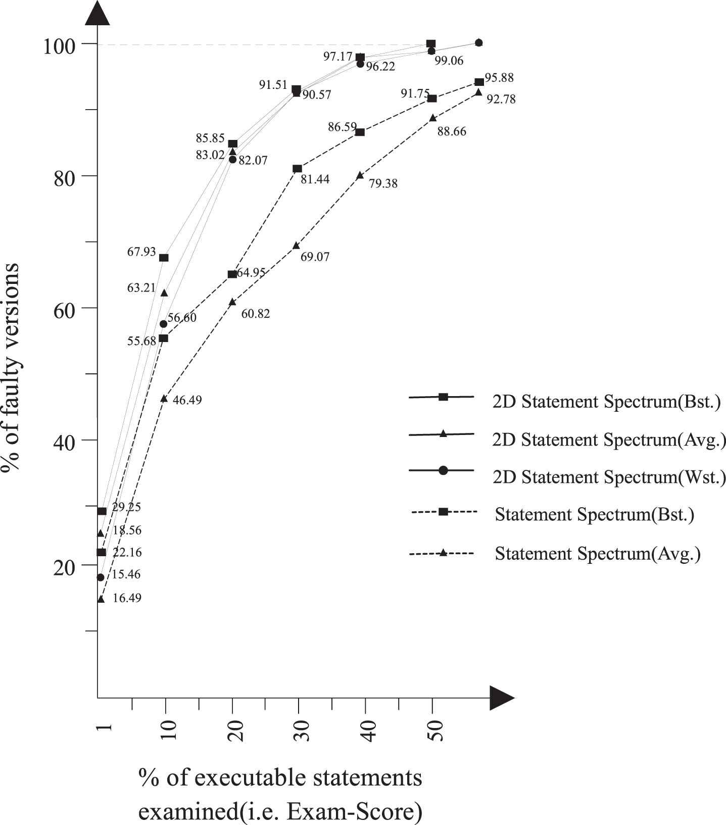
The Exam-Score comparison of two program spectrums.

The 2DSSBst can examine the maximum faulty versions at the Exam-Score of 1%, and our method results, both 2DSSBst and 2DSSAvg can always examine more faulty versions than SSBst does. As the Exam-Score exceeds 10%, our worst result 2DSSWst is better than SSBst and gets closer to 2DSSBst. And our method is able to examine the vast majority of faulty versions about more than 90% faulty versions when the Exam-Score is up to 30%, whereas the SSBst and SSAvg can’t examine 90% faulty versions until the Exam-Score is more than 50%. What’s more, the 2DSSAvg and 2DSSWst stay less than 5% faulty versions unexamined behind 2DSSBst when the Exam-Score is over about 15%, while the gap of faulty versions examined between SSBst and SSAvg can’t stay less than 5% faulty versions until the Exam-Score is up to 50%. Therefore, the 2DSS is more stable and efficient than statement spectrum in fault localization.

As the traditional statement spectrum only contains the features of statement execution states, many statements have the same suspiciousness as the faulty statement does. And only the faulty statement covered more by failure test cases and less by success test cases can be examined efficiently for statement spectrum. However, the contribution of 2DSS to fault localization is not only the statement execution states but also the Z-Score of each statement. The 2DSS refines the features of statements to reduce the number of statements with the same suspiciousness. In addition, the Z-Score is evaluated by data flow spectrum, and the statement with a larger ZF-Score is covered more by failure test cases in data flow spectrum, therefore, these statements covered more by failure test cases in statement spectrum or data flow spectrum can be examined efficiently for 2DSS, to be more precise, the 2DSS enhances the ability to detect faults for data dependency statements. Of course, if the fault isn’t in data dependency statements, there may be a slight decline in efficiency to locate the faulty statement as both ZF-Score and ZS-Score of the statement are zero.

Table 5

The percentage of faulty versions examined by SFL

Exam-Score (Avg.)	2DSFLF(Bst.)	2DSFLF(Avg.)	2DSFLF(Wst.)	BPNN	PPDG(Bst.)	Tarantula
0-1%	29.25%	25.47%	17.92%	6.56%	41.94%	13.93%
1%-10%	38.68%	37.74%	38.68%	43.44%	31.45%	41.80%
10%-20%	17.92%	19.81%	25.47%	24.59%	13.71%	5.74%
20%-30%	5.66%	7.55%	8.49%	11.48%	2.42%	9.84%
30%-40%	5.66%	6.60%	5.66%	7.38%	2.42%	8.20%
40%-50%	2.83%	1.89%	2.83%	3.28%	5.65%	7.38%
50%-100%	0.00%	0.94%	0.94%	3.28%	1.61%	13.12%

RQ2: How does the 2DSFLF perform on fault localization efficiency and precision with different activation functions?

Table 4

The percentage of faulty versions examined by 2DSFLF

Exam-Score (Avg.)	RBF	Linear	Sigmoid
0-1%	25.47%	18.87%	0.00%
1%-10%	37.74%	26.42%	18.87%
10%-20%	19.81%	19.81%	7.55%
20%-30%	7.55%	15.09%	2.83%
30%-40%	6.60%	6.60%	9.43%
40%-50%	1.89%	2.83%	16.04%
50%-100%	0.94%	10.38%	45.28%

Table 6 shows the percentage of faulty versions examined by 2DSFLF in different Exam-Score segments when different activation functions are applied in 2DSFLF fault localization model. The Exam-Score in the first column is divided into seven segments, for instance, 0-1% represents that the Exam-Score is less than or equal to 1%, and the segment 1%-10% represents the Exam-Score between 1% and 10%. In addition, for each segment, the left side is open interval and the right side is closed interval. The RBF in Eq. (6), Linear in Eq. (1) and Sigmoid in Eq. (11) of the table are three different activation functions. And these three functions are applied as the activation functions of 2DSFLF fault localizatin model respectively to locate the faults. And the Exam-Score in the table is the average Exam-Score of faulty versions.

Within the Exam-Score of 1%, 2DSFLF with RBF can examine 25.47% faulty versions, which examines 6.60% faulty versions more than 2DSFLF with Linear does, while 2DSFLF with Sigmoid cannot examine the faulty versions. Within the Exam-Score of 40%, 2DSFLF with RBF can examine the vast majority of faulty versions with only 2.83% faulty versions unexamined, and 2DSFLF with Linear can examine 86.79% faulty versions, while 2DSFLF with Sigmoid still cannot examine 61.32% faulty versions. Overall, the 2DSFLF with RBF has the best fault localization efficiency and precision, compared with the 2DSFLF with Linear or Sigmoid.

The activation functions Linear in Eq. (10) and Sigmoid in Eq. (11) map $X_{iitsc}$ to a new space by the inner product of vectors $< X_{i}$ , $U_{jitsc} >$ , whereas the RBF in Eq. (6) maps $X_{iitsc}$ to a new space by the euclidean distance $| | X_{i} - U_{j} | |$ of vectors which measures the similarity between the coverage of two test cases. Thus, the activation functions of the distance relationship between vectors like RBF perform better than the activation functions of the inner product relationship between two vectors in fault localization efficiency for our framework. $R_{ji} (X_{i}) = k * < X_{i}, U_{j} >$ (10) $R_{ji} (X_{i}) = \frac{1}{1 + \frac{1}{\exp (< X_{i}, U_{j} >)}}$ (11)

RQ3: How effective is 2DSFLF for fault localization compared to other SFLF?

Table 5 shows the faulty versions examined by various SFLF in seven segments of Exam-Score. Likewise, the fault localization efficiency of 2DSFLF in the best, average and worst Exam-Score for each faulty version are compared with the SFLF of BPNN, PPDG(Bst) and Tarantula whose experimental results have been reported in [27, 36]. In 0-1% of Exam-Score, the PPDG(Bst) has the best precision with 41.94% faulty versions examined, and all the results of our method 2DSFLF(Bst), 2DSFLF(Avg) and 2DSFLF(Wst) are better than those of other two methods BPNN and Tarantula. After 40% of Exam-Score, Only less than 4% faulty versions aren’t examined by our method, while the BPNN and PPDG(Bst) have about 7% faulty versions unexamined, and the result of Tarantula is the worst with 20.50% faulty versions unexamined.

Therefore, compared with PPDG(Bst), our method 2DSFLF improves about 5% faulty versions’ Exam-Score from more than 40% to less than 40%. The 2DSFLF(Bst) can examine all the faulty versions before the Exam-Score of 50%, while the others cannot. What’s more, the 2DSFLF has a greater fault localiztion precision than BPNN and Tarantula for more faulty versions can be examined in the interval 0-1% of Exam-Score, and is more efficient for more than 95% faulty versions can be examined in the Exam-Score range of 0-40%. Overall, the efficiency of 2DSFLF is relatively stable which can examine more than 90% faulty versions for all the results of our method before 30% of Exam-Score when the results of 2DSFLF in there cases the best, average and worst Exam-Score are compared.

Table 6 shows the comparison of the 2DSFLF and other methods whose results come from [15] about the Top-N and the Mean Exam-Score on Siemens Suit. At Top-1, 2DSFLF(Avg.) examines 22 faulty versions, which examines 11 more faulty versions than O^p does, and 2DSFLF(Avg.) examines 24 and 46 more faulty versions than O^p does at Top-3 and Top-10, though O^p examines more faulty versions than BPNN and Tarantula do at Top-1, Top-3 and Top-10. Hence, the 2DSFLF has a greater precision than other three methods. The Mean Exam-Score is the mean of the Exam-Score for all the faulty versions in the seven programs of Siemens Suit. As some inappropriate faulty versions presented in section 5.1 are discarded, these discarded versions are defined with a fairly poor Exam-Score of 80%, then take the Exam-Score of all the faulty versions into account to evaluate the Mean Exam-Score for 2DSFLF on Siemens Suit. And the ultimate results in Table 6 show that the 2DSFLF in the best, average and worst cases still has a smaller Mean Exam-Score, which means the 2DSFLF can examine the minimal statements to detect all the faulty versions on Siemens Suit, compared with other three methods, BPNN, Tarantula and O^p. In conclusion, compared with other SFLF, the 2DSFLF has the greatest efficiency and the second highest precision of fault localization on Siemens Suit.

Table 6

The precision and efficiency comparison of various methods

Method	Top-N			Mean
	@1	@3	@10	Exam-Score(%)
2DSFLF(Bst.)	27	43	74	28.72143
2DSFLF(Avg.)	22	37	74	29.26571
2DSFLF(Wst.)	12	30	60	30.09143
BPNN	10	13	25	40.48924
Tarantula	3	7	23	42.87242
O ^p	11	13	28	41.06086

6 Threats to validity

Some potential threats to the validity of our proposed approach are discussed in this section.

The generalization: Our framework 2DSFLF is only experimented on the Siemens Suit. It may not perform on other programs as effectively as the programs in the Siemens Suit. And the type of fault might have an impact on our framework’s fault localization efficiency. Especially, the faults of statement missing always lead to a bad efficiency, while the faults of mutation such as data mutation, operator mutation and so on usually can be examined efficiently. In addition, our framework is more suitable for analyzing the single-fault program, while the target program may have multiple faults in the real-world application scenario. Research [44, 45] also shows that the effectiveness of the existing SFLF decreases when a program contains multiple active faults due to interference between faults. Zakari et al. [46] proposed to use complex network theory to improve the efficiency of SFL formulas in multi-fault programs. The 2DSFLF may also use complex network theory to adapt to multi-fault localization.

The framework 2DSFLF: The data dependence definition of statements presented in section 3.1.2 needs further refinements to add more dependent statements to the data flow spectrum. This paper only defines the conversion of variable dependencies and function references to statement dependencies. However, the pointer and struct of C also have strong data dependence. In addition, our fault localization model composed of the RBF neural network and ridge regression performs efficiently in our framework, but the number of neurons and the selection of the kernel vectors in the second layer can also be further optimized. And a method for automatic model transformations [47, 48] based on prior knowledge is worthy of further study to improve the fault localization efficiency of 2DSFLF.

7 Conclusion and feature work

This paper proposes a fault localization framework 2DSFLF taking the 2DSS as training data and prove it efficient and high-precision in fault localization.

At first, the optimization spectrum 2DSS is compared with statement spectrum by experimenting on an empirical program ‘modify_mid’ and prove the 2DSFLF feasible. Subsequently, the fault localization framework 2DSFLF and the algorithm of 2DSFLF construction are given a detailed presentation. At last, the 2DSFLF is experimented on Siemens Suit around three research questions to draw three conclusions. The 2DSS obviously improves the fault localiztion efficiency for most faulty versions and is more efficient than statement spectrum. The activation function of RBF performs better than the activation functions which represent the inner product relationship between the input vector and kernel vector such as linear and sigmoid functions in our framework. And the 2DSFLF is the most efficient and has the second highest precision in fault localization compared to other SFLF. The 2DSFLF can examine about 97.17% faulty versions within the Exam-Score of 40%, which examines 3.73%, 4.43% and 17.67% faulty versions more than BPNN, PPDG and Tarantula do. The 2DSFLF can examine 74 faulty versions which is nearly three times as many as faulty versions examined by BPNN, Tarantula and O^p at Top-10, and examine about 11% fewer executable statements than them do when all the faulty versions are detected on the Siemens Suit.

Our future work will focus on refining the data dependence definition of statements and introducing more metrics to measure the eigenvalues of statements in 2DSS. In addition, our framework should be improved to accommodate multi-fault program localiztion.

References

Wright

C.S.

and Zia

T.A.

, A quantitative analysis into the economicsof correcting software bugs, 4th International Conference onComputational Intelligence in Security for InformationSystems(CISIS) 6694 (2011), 198–205.

Wong

W.E.

, Gao

R.Z.

, Abreu

, Li

Y.H.

and Wota Wa

, A survey onsoftware fault localization, IEEE Transactions on SoftwareEngineering 42(8) (2016), 707–740.

Pearson

, Campos

, Just

, Fraser

, Abreu

, Ernst

M.D.

, Pang

and Keller

, Evaluating and improving fault localization, 2017 IEEE/ACM 39th International Conference on Software Engineering (2017), 609–620.

Ren

S.B.

, Zhou

W.J.

, Zhou

H.W.

and Xia

, Weight prioritizedslicing based on constraint logic programming for faultlocalization, Plos One 15(4) (2020).

Ghorbani

and Flallah

M.S.

, Run-time verification for observational determinism using dynamic program slicing, International Conference on Information Security (2017), 405–416.

Mayer

and Stumptner

, Evaluating models for model based debugging, the 2008 23rd IEEE/ACM International Conference on Automated Software Engineering (2008), 128–137.

Pill

and Wotawa

, Exploiting observations from combinatorial testing for diagnostic reasoning, 30th International Workshop on Principles of Diagnosis (2019), 17–24.

Pill

and Quaritsch

, RC-Tree: A variant avoiding all the redundancy in Reiterąrs minimal hitting set algorithm, 2015 IEEE International Symposium on Software Reliability Engineering Workshops (2015), 78–84.

Kim

, Mun

, Yoo

and Kim

, Precise learn-to-rank faultlocalization using dynamic and static features of target programs, ACM Transactions on Software Engineering and Methodology 28(4) (2018), 1–34.

10.

Debroy

and Wong

W.E.

, Combining mutation and fault localizationfor automated program debugging, Journal of Systems andSoftware 90 (2014), 45–60.

11.

Liu

, Li

, Wang

L.X.

, Hu

Z.W.

and Zhao

R.L.

, Statement oriented mutant reduction strategy for mutation based fault localization, 2017 IEEE International Conference on Software Quality, Reliability and Security (2017), 126–137.

12.

Neelofar

, Naish

, Lee

and Ramamohanarao

, Improvingspectral-based fault localization using static analysis, Software-Practice & Experience 47(11) (2017), 1633–1655.

13.

Wang

R.C.

, Jiang

S.J.

, Zhang

and Yu

, Improving the accuracy of spectrum-based fault localization using multiple rules, IEICETransactions on Information and Systems E103D(6) (2020), 1328–1338.

14.

Wong

W.E.

, Debroy

, Golden

, Xu

X.F.

and Thuraisingham

, Effective software fault localization using an rbf neural network, IEEE Transactions on Reliability 61(1) (2012), 149–169.

15.

Heris

S.R.

and Keyvanpour

, Effectiveness of weighted neural network on accuracy of software fault localization, 2019 5th International Conference onWeb Research (ICWR) (2019), 100–104.

16.

Wong

W.E.

, Debroy

and Choi

, A family of code coverage basedheuristics for effective fault localization, Journal of Systemsand Software 83(2) (2010), 188–208.

17.

T.T.

, Dong

Y.W.

, Lau

M.F.

, Ng

, Chen

T.Y.

and Jiang

M.Y.

, Performance Analysis of Maximal Risk Evaluation Formulas for Spectrum-Based Fault Localization, Applied Sciences-basel 10(1) (2020).

18.

Tang

C.M.

, Chan

W.K.

, Yu

Y.T.

and Zhang

Z.Y.

, Accuracy Graphs of Spectrum-Based Fault Localization Formulas, IEEE Transactionson Reliability 66(2) (2017), 403–424.

19.

Keller

, Grunske

, Heiden

, Filieri

, van Hoorn

and Lo

, A critical evaluation of spectrum-based fault localization techniques on a large-scale software system, 2017 IEEE International Conference on Software Quality, Reliability and Security (2017), 114–125.

20.

Zhang

, Jiang

, Chan

W.K.

and Tse

T.H.

, Debugging through evaluation sequences: A controlled experimental study, 2008 32nd Annual IEEE International Computer Software and Applications Conference (2008), 128–135.

21.

H.L.

, Gao

, Huang

S.K.

and Wong

W.E.

, Spectrum base fault localization by exploiting the failure path, 2016 International Computer Symposium (2016), 252–257.

22.

Perez

, Abreu

and van Deursen

, A test-suite diagnosability metric for spectrum-based fault localization approaches, 2017 IEEE/ACM 39th International Conference on Software Engineering (2017), 654–664.

23.

, Zhang

Z.Y.

, Chan

W.K.

, Tse

T.H.

and Li

S.P.

, A generalnoise-reduction framework for fault localization of java programs, Information and Software Technology 55(5) (2013), 880–896.

24.

Masri

and Abou Assi

, Prevalence of coincidental correctness andmitigation of its impact on fault localization, ACMTransactions on Software Engineering and Methodology 23(1) (2014), 1–28.

25.

Zhang

, Yan

L.F.

, Zhang

Z.Y.

, Zhang

, Chan

W.K.

and Zhang

, Atheoretical analysis on cloning the failed test cases to improve spectrum-based fault localization, Journal of Systems andSoftware 129 (2017), 35–57.

26.

, Lin

M.X.

, Gao

, Zhang

and Zhang

X.Y.

, Locating faults using multiple spectra-specific models, ACM Symposium on Applied Computing (2011), 1404–1410.

27.

Jones

J.A.

and Harrold

M.J.

, Empirical evaluation of the tarantula automatic fault-localization technique, 2005 20th IEEE/ACM International Conference on Automated Software Engineering (2005), 273–282.

28.

Naish

, Lee

H.J.

and Ramamohanarao

, A model for spectra-basedsoftware diagnosis, Engineering and Methodology 20(3) (2011), 1–32.

29.

Wong

W.E.

, Debroy

and Xu

D.X.

, Towards better fault localization:A crosstab-based statistical approach, IEEE Transactions onSystems Man and Cybernetics Part C-Applications and Reviews 42(3) (2012), 378–396.

30.

Steimann

, Frenkel

and Abreu

, Threats to the validity and value of empirical assessments of the accuracy of coveragebased fault locators, 2013 International Symposium on Software Testing and Analysis (2013), 314–324.

31.

Wong

W.E.

, Debroy

, Gao

R.Z.

and Li

Y.H.

, The dstar method foreffective software fault localization, IEEE Transactions onReliability 63(1) (2014), 290–308.

32.

Zhang

, Li

Z.J.

and Yang

, Improving Fault-Localization Accuracyby Referencing Debugging History to Alleviate Structure Bias in CodeSuspiciousness, IEEE Transactions on Reliability 69(3) (2020), 1021–1049.

33.

Neelofar

, Naish

and Ramamohanarao

, Spectral-based faultlocalization using hyperbolic function, Software-practice &Experience 48(3) (2018), 641–664.

34.

Sohn

and Yoo

, FLUCCS: Using code and change metrics to improve fault localization, 26th ACM SIGSOFT International Symposium on Software Testing and Analysis (2017), 273–283.

35.

Zhang

M.S.

, Li

, Zhang

L.M.

and Khurshid

, Boosting Spectrum-Based Fault Localization using Page Rank, 26th ACM SIGSOFT International Symposium on Software Testing and Analysis (2017), 261–272.

36.

Baah

G.K.

, Podgurski

and Harroldi

M.J.

, The probabilistic programdependence graph and its application to fault diagnosis, IEEETransactions on Software Engineering 36(4) (2010), 528–545.

37.

Wong

W.E.

and Qi

, Bp neural network-based effective faultlocalization, International Journal of Software Engineering andKnowledge Engineering 19(4) (2009), 573–597.

38.

Zheng

, Hu

D.S.

and Wang

, Fault localization analysis based ondeep neural network, Mathematical Problems in Engineering 2016 (2016).

39.

Wang

, Huang

Z.Q.

, Wang

R.C.

and Yu

, Spectrum-Based FaultLocalization Using Fault Triggering Model to Refine Fault RankingList IEICE Transactions on Information and Systems E101D(10) (2018), 2436–2446.

40.

Cui

Z.Q.

, Jia

M.H.

, Chen

, Zheng

L.W.

and Liu

X.L.

, ImprovingSoftware Fault Localization by Combining Spectrum and Mutation, IEEE Access 8 (2020), 172296–172307.

41.

, Song

, Gong

G.Q.

, Zhou

S.W.

and Lv

, A multitechniquefusion approach for fault localization in manufacturing software, Journal of Intelligent & Fuzzy Systems 38(1) (2020), 229–238.

42.

Silva

, Leitao

P.S.

, Dantas

, Camilo

C.G.

and Harrison

, Data-flow-based evolutionary fault localization, The 35th Annual ACM Symposium on Applied Computing (2020), 1963–1970.

43.

Masri

and Podgurski

, Measuring the strength of informationflows in programs, ACM Transactions on Software Engineering andMethodology 19(2) (2009), 1–33.

44.

DiGiuseppe

and Jones

J.A.

, Fault density, fault types, andspectra-based fault localization, Empirical SoftwareEngineering 20(4) (2015), 928–967.

45.

Yan

X.B.

, Liu

and Li

J.X.

, The failure behaviors of multifaults programs: An empirical study, 2017 IEEE International Conference on Software Quality, Reliability And Security Compantion (2017), 1–7.

46.

Zakari

, Lee

S.P.

and Chong

C.Y.

, Simultaneous Localization ofSoftware Faults Based on Complex Network Theory, IEEE Access 6 (2018), 23990–24002.

47.

Troya

, Segura

, Parejo

J.A.

and Ruiz-Cortes

, Spectrum-Based Fault Localization in Model Transformations, ACM Transactionson Software Engineering and Methodology 27(3) (2018).

48.

P.F.

, Jiang

M.Y.

and Ding

Z.H.

, Fault Localization With WeightedTest Model in Model Transformations, IEEE Access 8(2020), 14054–14064.