A framework of decision making based on bipolar fuzzy competition hypergraphs

Abstract

Bipolarity plays a key role in different domains such as technology, social networking and biological sciences for illustrating real-world phenomenon using bipolar fuzzy models. In this article, novel concepts of bipolar fuzzy competition hypergraphs are introduced and discuss the application of the proposed model. The main contribution is to illustrate different methods for the construction of bipolar fuzzy competition hypergraphs and their variants. Authors study various new concepts including bipolar fuzzy row hypergraphs, bipolar fuzzy column hypergraphs, bipolar fuzzy k -competition hypergraphs, bipolar fuzzy neighborhood hypergraphs and strong hyperedges. Besides, we develop some relations between bipolar fuzzy k -competition hypergraphs and bipolar fuzzy neighborhood hypergraphs. Moreover, authors design an algorithm to compute the strength of competition among companies in business market. A comparative analysis of the proposed model is discuss with the existing models such bipolar fuzzy competition graphs and fuzzy competition hypergraphs.

Keywords

Bipolar fuzzy competition hypergraphs bipolar fuzzy neighborhood hypergraphs

1 Introduction

In 1968, Cohen [7] introduced the idea of competition graphs that arose on competition between species in an ecosystem. It has a remarkable origin to show the explicit behaviors of objects and especially predator-prey relations. Competition graphs have been applicable in different research areas of scientific and technical knowledge. Many researchers studied competition graphs and their variants after inspiration of food competition in food webs between species. But in all this work, the theory of competition graphs do not describe the competition or relations between three or more objects. To solve this problem, the concept of competition hypegraphs introduced by Sonntag and Teichert [27] in 2004. These are crisp hypergraphs in which nodes and edges are explicitly defined. However, to deal with uncertainty and to describe all real-world competitions including predator-prey relations, powerful communities in a social network, rivalries in the business market, signal influence of wireless devices, the notion of fuzzy sets has been applied in competition hypergraphs.

The theory of fuzzy sets introduced by Zadeh [30] in order to discuss the phenomena of vagueness and uncertainty in various real-life problems. Pawlak [14] introduced the notion of rough sets to express vagueness in terms of a boundary region of a set. Dubois and prade [8] obtained two different hybrid models: fuzzy rough sets and rough fuzzy sets by combining the techniques of rough and fuzzy sets. Zhang et al. [34] discussed multi-criteria decision-making method based on a fuzzy rough set model with fuzzy α-neighborhoods. Moreover, Ye et al. [29] discussed fuzzy rough set model with fuzzy operators. Based on Zadeh’s [31] fuzzy relations, Kaufmann [10] defined the notion of a fuzzy graph in 1973. Another elaborated definition of a fuzzy graph and the fuzzy relations between sets were studied by Rosenfeld [17] in 1975. Moreover, some remarkable results on fuzzy graphs were introduced by Bhattacharya [6], Mordeson and Nair [13] studied certain operations on fuzzy graphs. The concept of fuzzy hypergraphs was extended and redefined by Lee-Kwang and Lee [11]. The notions of fuzzy p-competition graphs and fuzzy k-competition graphs were studied by Samanta and Pal [18]. Whang et al. [28] presented three way multi-attribute decision making under hesitant fuzzy environments. Zhan et al. [35] studied three way multi-attribute decision-making based on outranking relations.

The idea of bipolar fuzzy (BF) sets was introduced by Zhang [33]. Bipolar fuzzy sets capture the opposite sided facts positive facts and negative facts of human perceptions. Al-shehri and Akram [5] initiated the concept of bipolar fuzzy competition graphs. Sarwar and Akram [22, 23] extended the concept of bipolar fuzzy competition graphs and introduced certain types of bipolar fuzzy competition graphs, bipolar fuzzy neighborhood graphs and presented algorithm to compute the strength of competition in real-world problems of competitive networks. Bipolar fuzzy sets have numerous applications including artificial intellect, information technology, and social science etc. In real-world problems competitions and relations in which opposite side facts arise the theory of fuzzy competition hypergraphs is inadequate. For example, in predator-prey relations, a species may be healthy and unhealthy, the prey is beneficial and harmful at a time and these are bipolar fuzzy facts. This idea forces us to apply the concept of bipolar fuzzy sets to fuzzy competition hypergraphs. We have used some basic concepts and terminologies in this article. For other concepts and terminologies that are not specified in this paper, we refer the reader to [1–4 , 32].

The motives of this study are as follows:

Fuzzy sets are used for depicting vagueness, uncertainty, and approximate reasoning that occur in real-world problems. However, to deal with human decision making that is based on bipolar judgemental thinking this theory is inadequate. The powerful technique of bipolar fuzziness has the ability to overcome this difficulty and obtain more accurate results.

Competition hypergraphs used (where information is explicit) to describe the real-world competitions and where information is vague we apply the model of fuzzy competition hypergraphs. Due to occurrence of bipolar facts, this theory is not enough to sort out all real-life competitions. The framework of bipolar fuzzy competition hypergraphs plays an important part to overwhelm this difficulty and it is successfully manipulated in different research areas.

The main contribution of this study is as follows:

The notions of bipolar fuzzy competition hypergraphs of a bipolar fuzzy digraphs, bipolar fuzzy row hypergraphs, bipolar fuzzy column hypergraphs, bipolar fuzzy k -competition hypergraphs, bipolar fuzzy open neighborhood hypergraphs, bipolar fuzzy closed neighborhood hypergraphs, strong hyperedges are discuss in this article. Various powerful techniques for construction of bipolar fuzzy competition hypergraphs and their variants are also investigated.

The significance of given notions is study with an application in the business market and an algorithm is design to compute the strength of competition among the vertices. Moreover, the comparison of bipolar fuzzy competition hypergraphs with bipolar fuzzy competition graphs and fuzzy competition hypergraphs are discuss in this paper.

The structure of this paper is as follows:

Section 2 gives some important preliminaries related to this study.

Section 3 describes bipolar fuzzy competition hypergraphs and their variants with suitable examples. Also gives some results relates to strong hyperedges.

Section 4 establishes the notions of bipolar fuzzy open neighborhood hypergraphs, bipolar fuzzy closed neighborhood hypergraphs, bipolar fuzzy k-competition hypergraphs.

Section 5 propose a decision-making method that takes advantage of our theoretical framework and shows how to apply the notion of bipolar fuzzy competition hypergraphs in the business market.

Section 6 gives the comparison of bipolar fuzzy competition hypergraphs with bipolar fuzzy competition graphs and fuzzy competition hypergraphs.

The conclusion is written in Section 7.

2 Preliminaries

Let Y be a non-empty set. A crisp graph $D^{*}$ on Y is a pair (Y, W) , where Y is called vertex set and W ⊆ Y × Y is called edge set. A competition graph $K$ = (Y, E) of a digraph $\vec{D}$ = $(Y, \vec{W})$ containing the vertex set same as in $\vec{D}$ and there is an edge between two vertices y₁ and y₂ iff $\vec{y_{1} y}, \vec{y_{2} y} \in \vec{W}$ for some y ∈ Y .

Definition 2.1. [4] A bipolar fuzzy digraph on Y is a pair $\vec{J}$ = $(M, \vec{N}),$ where M = $(η_{M}^{+}, η_{M}^{-})$ is a bipolar fuzzy set on Y and $\vec{N}$ = $(η_{\vec{N}}^{+}, η_{\vec{N}}^{-})$ is a bipolar fuzzy relation on Y with the property that $η_{\vec{N}}^{+} (y_{1} y_{2}) ⩽ η_{M}^{+} (y_{1}) \land η_{M}^{+} (y_{2})$ and $η_{\vec{N}}^{-} (y_{1} y_{2}) ⩾ η_{M}^{-} (y_{1}) \lor η_{M}^{-} (y_{2}),$ for all y₁, y₂ ∈ Y .

Definition 2.2. [21] A bipolar fuzzy hypergraph on Y is a pair H = (M, R) , where M = {M₁, M₂, ⋯ , M_r} is a family of bipolar fuzzy subsets on Y such that ⋃_isupp(M_i) = Y, for all M_i ∈ M. $R = (η_{R}^{+}, η_{R}^{-})$ is a bipolar fuzzy relation on the bipolar fuzzy subsets $M_{i} = (η_{M_{i}}^{+}, η_{M_{i}}^{-})$ such that $\begin{matrix} η_{R}^{+} (E_{i}) & = & η_{R}^{+} ({y_{1}, y_{2}, \dots, y_{p}}) \\ \leq \min {η_{M_{i}}^{+} (y_{1}), η_{M_{i}}^{+} (y_{2}), \dots, η_{M_{i}}^{+} (y_{p})}, \\ η_{R}^{-} (E_{i}) & = & η_{R}^{-} ({y_{1}, y_{2}, \dots, y_{p}}) \\ \geq \max {η_{M_{i}}^{-} (y_{1}), η_{M_{i}}^{-} (y_{2}), \dots, η_{M_{i}}^{-} (y_{p})}, \end{matrix}$ for all y₁, y₂, ⋯ , y_p ∈ Y .

Definition 2.3. [23] A bipolar fuzzy out neighborhood of a vertex y in a bipolar fuzzy digraph $\vec{J} = (M, \vec{N})$ is a bipolar fuzzy set $N^{+} (y) = (Y_{y}^{+}, η_{N^{+} (y)}^{+}, η_{N^{+} (y)}^{-}),$ where $Y_{y}^{+} = {y_{1} \in Y | η_{\vec{N}}^{+} ({yy}_{1}) > 0, η_{\vec{N}}^{-} ({yy}_{1}) < 0}$ and $η_{N^{+} (y)}^{+} : Y_{y}^{+} ⟶ [0, 1]$ and $η_{N^{+} (y)}^{-} : Y_{y}^{+} ⟶ [- 1, 0]$ are defined by $η_{N^{+} (y)}^{+} (y_{1}) = η_{\vec{N}}^{+} ({yy}_{1})$ and $η_{N^{+} (y)}^{-} (y_{1}) = η_{\vec{N}}^{-} ({yy}_{1})$ .

Definition 2.4. [23] A bipolar fuzzy in neighborhood of a vertex y in a bipolar fuzzy digraph $\vec{J} = (M, \vec{N})$ is a bipolar fuzzy set $N^{-} (y) = (Y_{y}^{-}, η_{N^{-} (y)}^{+}, η_{N^{-} (y)}^{-}),$ where $Y_{y}^{-} = {y_{1} \in Y | η_{\vec{N}}^{+} (y_{1} y) > 0, η_{\vec{N}}^{-} (y_{1} y) < 0}$ and $η_{N^{-} (y)}^{+} : Y_{y}^{-} ⟶ [0, 1]$ and $η_{N^{-} (y)}^{-} : Y_{y}^{-} ⟶ [- 1, 0]$ are defined by $η_{N^{-} (y)}^{+} (y_{1}) = η_{\vec{N}}^{+} (y_{1} y)$ and $η_{N^{-} (y)}^{-} (y_{1}) = η_{\vec{N}}^{-} (y_{1} y)$ .

Definition 2.5. [23] A bipolar fuzzy open neighborhood of a vertex z of a bipolar fuzzy graph $J = (M, N)$ is a bipolar fuzzy set $N (z) = (Z_{z}, η_{N (z)}^{+}, η_{N (z)}^{-}),$ where $Z_{z} = {z_{1} | η_{N}^{+} ({zz}_{1}) > 0, η_{N}^{-} ({zz}_{1}) < 0}$ and $η_{N (z)}^{+} : Z_{z} ⟶ [0, 1]$ and $η_{N (y)}^{-} : Z_{z} ⟶ [- 1, 0]$ are defined by $η_{N (z)}^{+} (z_{1}) = η_{N}^{+} ({zz}_{1})$ and $η_{N (z)}^{-} (z_{1}) = η_{N}^{-} ({zz}_{1})$ .

Definition 2.6. [23] A bipolar fuzzy closed neighborhood of a vertex z of a bipolar fuzzy graph $J = (M, N)$ is a bipolar fuzzy set defined as $N [z] = N (z) \cup {z, η_{M}^{+} (z), η_{M}^{-} (z)}$ .

Definition 2.7. [23] The underlying bipolar fuzzy graph of a bipolar fuzzy digraph $\vec{J} = (M, \vec{N})$ is a bipolar fuzzy graph $U (\vec{J}) = (M, N),$ where $N = (η_{N}^{+}, η_{N}^{-})$ is defined as N (y₁y₂) = ${\begin{matrix} (η_{\vec{N}}^{+} (y_{1} y_{2}), η_{\vec{N}}^{-} (y_{1} y_{2})), & if \vec{y_{1} y_{2}} \in \vec{E}, \vec{y_{2} y_{1}} \notin \vec{E} \\ (η_{\vec{N}}^{+} (y_{2} y_{1}), η_{\vec{N}}^{-} (y_{2} y_{1})), & if \vec{y_{2} y_{1}} \in \vec{E}, \vec{y_{1} y_{2}} \notin \vec{E} \\ (η_{\vec{N}}^{+} (y_{1} y_{2}) \land η_{\vec{N}}^{+} (y_{2} y_{1}), η_{\vec{N}}^{-} (y_{1} y_{2}) \lor η_{\vec{N}}^{-} (y_{2} y_{1})), & if \vec{y_{1} y_{2}}, \vec{y_{2} y_{1}} \in \vec{E} \end{matrix}$ where $\vec{E} = supp (\vec{N})$ .

The symbols used in this article are given in Table 1.

Table 1
List of symbols

Symbols Description

$J$ BF graph

$\vec{J}$ BF digraph

$C (\vec{J})$ BF competition graph

$CH (\vec{J})$ BF competition hypergraph

$CEH (\vec{J})$ BF common enemy hypergraph

$R \circ H (A)$ BF row hypergraph

$C \circ H (A)$ BF column hypergraph

$DCH (\vec{J})$ BF double competition hypergraph

$NH (\vec{J})$ BF niche hypergraph

$C_{k} (\vec{J})$ BF k -competition hyperegraph

$C_{k} E (\vec{J})$ BF k -common enemy hyperegraph

$N (J)$ BF open-neighborhood hypergraph

$N [J]$ BF closed-neighborhood hypergraph

Symbols	Description
$J$	BF graph
$\vec{J}$	BF digraph
$C (\vec{J})$	BF competition graph
$CH (\vec{J})$	BF competition hypergraph
$CEH (\vec{J})$	BF common enemy hypergraph
$R \circ H (A)$	BF row hypergraph
$C \circ H (A)$	BF column hypergraph
$DCH (\vec{J})$	BF double competition hypergraph
$NH (\vec{J})$	BF niche hypergraph
$C_{k} (\vec{J})$	BF k -competition hyperegraph
$C_{k} E (\vec{J})$	BF k -common enemy hyperegraph
$N (J)$	BF open-neighborhood hypergraph
$N [J]$	BF closed-neighborhood hypergraph

3 Bipolar fuzzy competition hypergraphs

In this section, we define BF competition hypergraphs and their variants with suitable examples. Also discuss some results related to strong hyperedges.

Definition 3.1. Let $\vec{J} = (M, \vec{N})$ be a BF digraph on Y . The BF competition hypergraph $CH (\vec{J}) = (M, R)$ corresponding to $\vec{J}$ containing the BF vertex set same as in BF digraph $\vec{J}$ and E = {y₁, y₂, ⋯ , y_p} ⊆ Y is a hyperedge of $CH (\vec{J})$ if N ⁺ (y₁)∩ N ⁺ (y₂) ∩ ⋯ ∩ N ⁺ (y_p) ≠ ∅. The positive and negative membership degree of the hyperedge E = {y₁, y₂, ⋯ , y_p} are defined as $\begin{matrix} η_{R}^{+} (E) & = & [η_{M}^{+} (y_{1}) \land η_{M}^{+} (y_{2}) \land \dots \land η_{M}^{+} (y_{p})] \\ \times h (N^{+} (y_{1}) \cap N^{+} (y_{2}) \cap \dots \cap N^{+} (y_{p})), \\ η_{R}^{-} (E) & = & [η_{M}^{-} (y_{1}) \lor η_{M}^{-} (y_{2}) \lor \dots \lor η_{M}^{-} (y_{p})] \\ \times h (N^{+} (y_{1}) \cap N^{+} (y_{2}) \cap \dots \cap N^{+} (y_{p})), \end{matrix}$ where h (N ⁺ (y₁) ∩ N ⁺ (y₂) ∩ ⋯ ∩ N ⁺ (y_p)) indicates the height of a BF set.

The procedure is given in Algorithm 3.1 for computing BF competition hyperedge $CH (\vec{J})$ of a BF digraph $\vec{J} .$

Algorithm 3.1. Method for construction of BF competition hypergraph

The adjacency matrix A = [y_ij] _n×n of a BF digraph $\vec{J} = (M, \vec{N})$ such that $\vec{N} (y_{i} y_{j}) = (η_{\vec{N}}^{+} (y_{i} y_{j}), η_{\vec{N}}^{-} (y_{i} y_{j})) = (y_{ij}^{+}, y_{ij}^{-})$ as shown in Table 2.

Define a relation f : Y ⟶ Y by f (y_i)=y_j if $y_{ij}^{+} > 0$ and $y_{ij}^{-} < 0$ .

Determine the family of sets Z = {E_i = f ^-1 (y_i) : |f ^-1 (y_i) |≥2, y_i ∈ Y} , where E_i = {y_i
₁, y_i
₂, ⋯ , y_{i
_r}} is a hyperedge of $CH (\vec{J})$ .

Compute the grade of membership of each hyperedge by using Definition 3.1.

Table 2
Adjacency matrix

A y ₁ y ₂ ⋯ y _n

y ₁ $(y_{11}^{+}, y_{11}^{-})$ $(y_{12}^{+}, y_{12}^{-})$ ⋯ $(y_{1 n}^{+}, y_{1 n}^{-})$

y ₂ $(y_{21}^{+}, y_{21}^{-})$ $(y_{22}^{+}, y_{22}^{-})$ ⋯ $(y_{2 n}^{+}, y_{2 n}^{-})$

⋮ ⋮ ⋮ ⋱ ⋮

y _n $(y_{n 1}^{+}, y_{n 1}^{-})$ $(y_{n 2}^{+}, y_{n 2}^{-})$ ⋯ $(y_{nn}^{+}, y_{nn}^{-})$

A	y ₁	y ₂	⋯	y _n
y ₁	$(y_{11}^{+}, y_{11}^{-})$	$(y_{12}^{+}, y_{12}^{-})$	⋯	$(y_{1 n}^{+}, y_{1 n}^{-})$
y ₂	$(y_{21}^{+}, y_{21}^{-})$	$(y_{22}^{+}, y_{22}^{-})$	⋯	$(y_{2 n}^{+}, y_{2 n}^{-})$
⋮	⋮	⋮	⋱	⋮
y _n	$(y_{n 1}^{+}, y_{n 1}^{-})$	$(y_{n 2}^{+}, y_{n 2}^{-})$	⋯	$(y_{nn}^{+}, y_{nn}^{-})$

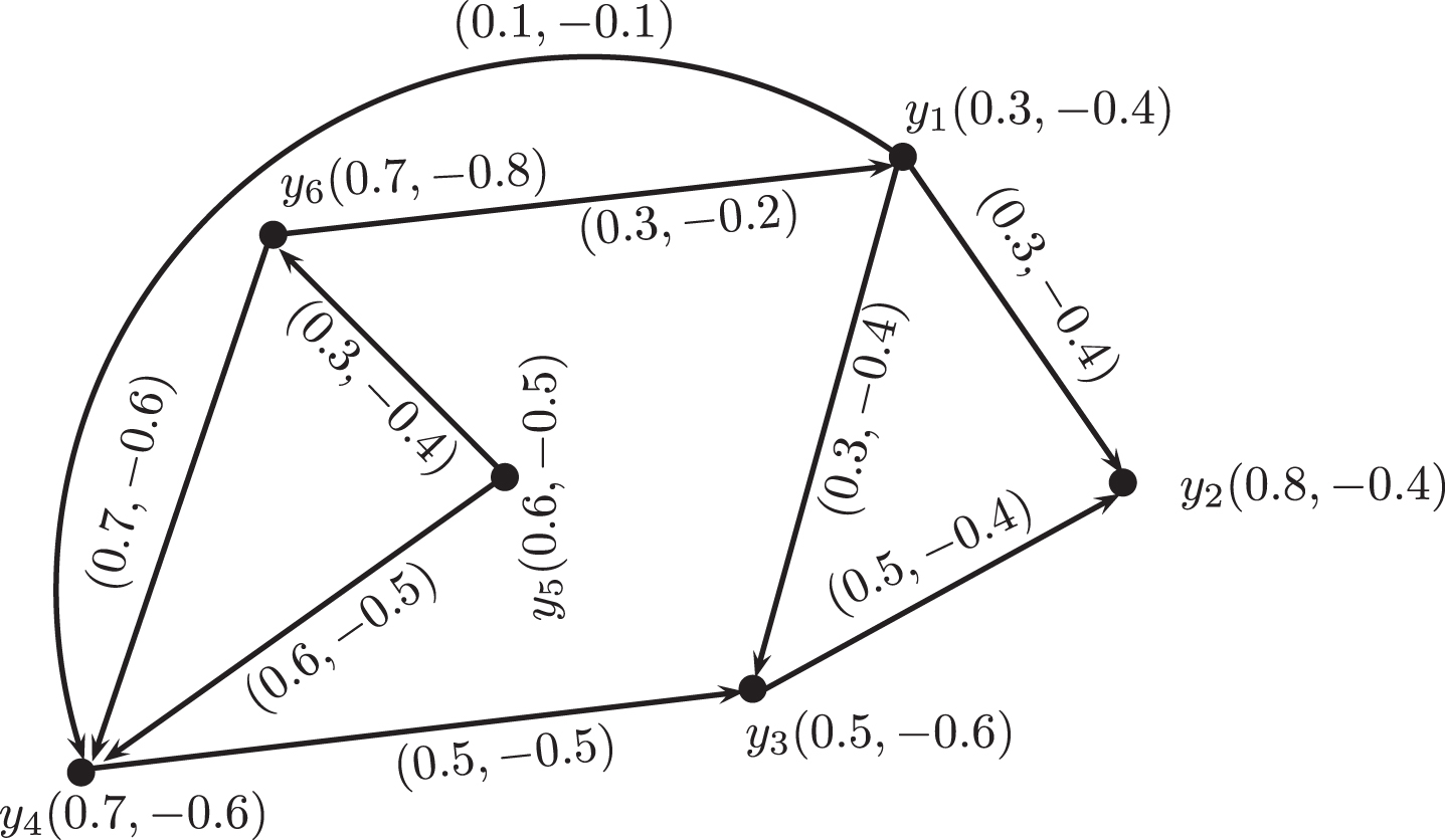
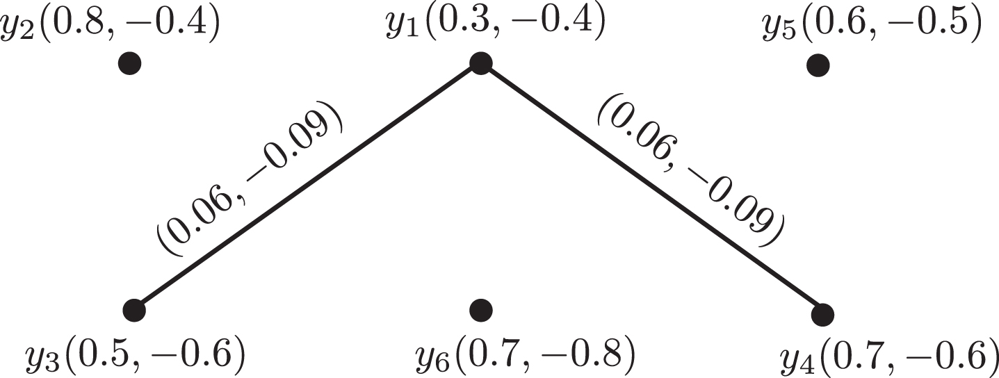
Example 3.2. Consider the set Y = {y₁, y₂, y₃, y₄, y₅, y₆}. Let M is a BF set on Y and $\vec{N}$ is a BF relation in Y as shown in Table 3 and 4, respectively.

Table 3

BF vertex set M

y	$(η_{M}^{+}, η_{M}^{-})$	y	$(η_{M}^{+}, η_{M}^{-})$
y ₁	(0.3, - 0.4)	y ₄	(0.7, - 0.6)
y ₂	(0.8, - 0.4)	y ₅	(0.6, - 0.5)
y ₃	(0.5, - 0.6)	y ₆	(0.7, - 0.8)

Table 4

BF relation $\vec{N}$

y	$(η_{\vec{N}}^{+}, η_{\vec{N}}^{-})$	y	$(η_{\vec{N}}^{+}, η_{\vec{N}}^{-})$
$\vec{y_{1} y_{2}}$	(0.3, - 0.4)	$\vec{y_{1} y_{3}}$	(0.3, - 0.4)
$\vec{y_{1} y_{4}}$	(0.1, - 0.1)	$\vec{y_{3} y_{2}}$	(0.5, - 0.4)
$\vec{y_{4} y_{3}}$	(0.5, - 0.5)	$\vec{y_{5} y_{6}}$	(0.3, - 0.4)
$\vec{y_{5} y_{4}}$	(0.6, - 0.5)	$\vec{y_{6} y_{1}}$	(0.3, - 0.2)
$\vec{y_{6} y_{4}}$	(0.7 - 0.6)

The BF digraph $\vec{J} = (M, \vec{N})$ on Y is given in Figure 3.1.

Fig. 3.1

BF digraph $\vec{J}$

The BF out neighborhood of all vertices in $\vec{J}$ are specified in Table 5.

Table 5

BF out neighborhood of vertices in $\vec{J}$

y ∈ Y	N⁺ (y)
y ₁	{(y₂, 0.3, - 0.4) , (y₃, 0.3, - 0.4) , (y₄, 0.1, - 0.1)}
y ₂	∅
y ₃	{(y₂, 0.5, - 0.4)}
y ₄	{(y₃, 0.5, - 0.5)}
y ₅	{(y₄, 0.6, - 0.5) , (y₆, 0.3, - 0.4)}
y ₆	{(y₁, 0.3, - 0.2) , (y₄, 0.7, - 0.6)}

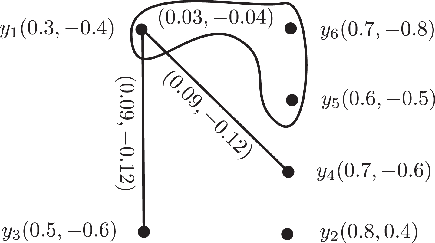
Using Algorithm 3.1, the relation f : Y ⟶ Y is given in Figure 3.2. Using relation given in Figure 3.2, there are three hyperedges f ^-1 (y₂) = E₂ = {y₁, y₃}, f ^-1 (y₃) = E₃ = {y₁, y₄} , and f ^-1 (y₄) = E₄ = {y₁, y₅, y₆} of $CH (\vec{J})$ . Now we calculate the membership grade of each hyperedge of $CH (\vec{J})$ . $\begin{matrix} η_{R}^{+} (E_{2}) & = & [η_{M}^{+} (y_{1}) \land η_{M}^{+} (y_{3})] \times h (N^{+} (y_{1}) \\ \cap N^{+} (y_{3})) = 0.3 \times 0.3 = 0.09, \\ η_{R}^{-} (E_{2}) & = & [η_{M}^{-} (y_{1}) \lor η_{M}^{-} (y_{3})] \times h (N^{+} (y_{1}) \\ \cap N^{+} (y_{3})) = - 0.4 \times 0.3 = - 0.12 . \\ η_{R}^{+} (E_{3}) & = & [η_{M}^{+} (y_{1}) \land η_{M}^{+} (y_{4})] \times h (N^{+} (y_{1}) \\ \cap N^{+} (y_{4})) = 0.3 \times 0.3 = 0.09, \\ η_{R}^{-} (E_{3}) & = & [η_{M}^{-} (y_{1}) \lor η_{M}^{-} (y_{4})] \times h (N^{+} (y_{1}) \\ \cap N^{+} (y_{4})) = - 0.4 \times 0.3 = - 0.12 . \\ η_{R}^{+} (E_{4}) & = & [η_{M}^{+} (y_{1}) \land η_{M}^{+} (y_{5}) \land η_{M}^{+} (y_{6})] \\ \times h (N^{+} (y_{1}) \cap N^{+} (y_{5}) \cap N^{+} (y_{6})) \\ = 0.3 \times 0.1 = 0.03, \\ η_{R}^{-} (E_{4}) & = & [η_{M}^{-} (y_{1}) \lor η_{M}^{-} (y_{5}) \lor η_{M}^{-} (y_{6})] \\ \times h (N^{+} (y_{1}) \cap N^{+} (y_{5}) \cap N^{+} (y_{6})) \\ = - 0.4 \times 0.1 = - 0.04 . \end{matrix}$ The BF competition hypergraph is given in Figure 3.3.

Fig. 3.2

Representation of BF relation in $\vec{J}$

Fig. 3.3

$CH (\vec{J})$

Definition 3.3. Let $\vec{J} = (M, \vec{N})$ be a BF digraph on Y . The BF common enemy hypergraph $CEH (\vec{J}) = (M, S)$ corresponding to $\vec{J}$ containing the BF vertex set same as in BF digraph $\vec{J}$ and E = {y₁, y₂, ⋯ , y_p} ⊆ Y is a hyperedge of $CEH (\vec{J})$ if N ^- (y₁) ∩ N ^- (y₂) ∩ ⋯ ∩ N ^- (y_p) ≠ ∅ . The membership grade of the hyperedge E = {y₁, y₂, ⋯ , y_p} is defined as $\begin{matrix} η_{S}^{+} (E) & = & [η_{M}^{+} (y_{1}) \land η_{M}^{+} (y_{2}) \land \dots \land η_{M}^{+} (y_{p})] \\ \times h (N^{-} (y_{1}) \cap N^{-} (y_{2}) \cap \dots \cap N^{-} (y_{p})), \\ η_{S}^{-} (E) & = & [η_{M}^{-} (y_{1}) \lor η_{M}^{-} (y_{2}) \lor \dots \lor η_{M}^{-} (y_{p})] \\ \times h (N^{-} (y_{1}) \cap N^{-} (y_{2}) \cap \dots \cap N^{-} (y_{p})) . \end{matrix}$

The method for computing BF common enemy hypergraph $CEH (\vec{J})$ of a BF digraph $\vec{J}$ is explained in Algorithm 3.2.

Algorithm 3.2. Method for the construction of BF common enemy hypergraph

Follow first step of Algorithm 3.1.

Define a relation f : Y ⟶ Y by f (y_i)=y_j if $y_{ij}^{+} > 0$ and $y_{ij}^{-} < 0$ .

Determine the family of sets Z = {E_i = f (y_i) : |f (y_i) |≥2, y_i ∈ Y} , where E_i = {y_i
₁, y_i
₂, ⋯ , y_{i
_r}} is a hyperedge of $CEH (\vec{J})$ .

Compute the grade of membership of each hyperedge by using Definition 3.3.

Example 3.4. Consider the BF digraph $\vec{J} = (M, \vec{N})$ as given in Figure 3.1. The BF in neighborhood of all vertices in $\vec{J}$ are given in Table 6.

Table 6

BF in neighborhood of vertices in $\vec{J}$

y ∈ Y	N^- (y)
y ₁	{(y₆, 0.3, - 0.2)}
y ₂	{(y₁, 0.3, - 0.4) , (y₃, 0.5, - 0.4)}
y ₃	{(y₁, 0.3, - 0.4) , (y₄, 0.5, - 0.5)}
y ₄	{(y₁, 0.1, - 0.1) , (y₅, 0.6, - 0.5) , (y₆, 0.7, - 0.6)}
y ₅	∅
y ₆	{(y₅, 0.3, - 0.4)}

By using Algorithm 3.2, there are three hyperedges f (y₁) = E₁ = {y₂, y₃, y₄}, f (y₅) = E₅ = {y₄, y₆} , and f (y₆) = E₆ = {y₁, y₄} of $CEH (\vec{J})$ . Now we calculate the membership grade of each hyperedge of $CEH (\vec{J})$ . $\begin{matrix} η_{S}^{+} (E_{1}) & = & [η_{M}^{+} (y_{2}) \land η_{M}^{+} (y_{3}) \land η_{M}^{+} (y_{4})] \\ \times h (N^{-} (y_{2}) \cap N^{-} (y_{3}) \cap N^{-} (y_{4})) \\ = 0.5 \times 0.1 = 0.05, \\ η_{S}^{-} (E_{1}) & = & [η_{M}^{-} (y_{2}) \lor η_{M}^{-} (y_{3}) \lor η_{M}^{-} (y_{4})] \\ \times h (N^{-} (y_{2}) \cap N^{-} (y_{3}) \cap N^{-} (y_{4})) \\ = - 0.4 \times 0.1 = - 0.04 . \end{matrix}$ Similarly, $η_{S}^{+} (E_{5}) = 0.21$ and $η_{S}^{-} (E_{5}) = - 0.18$ , $η_{S}^{+} (E_{6}) = 0.09$ and $η_{S}^{-} (E_{6}) = - 0.12$ . The BF common enemy hypergraph is given in Figure 3.4.

Fig. 3.4

$CEH (\vec{J})$

Definition 3.5. Let A = [y_ij] _n×n be the adjacency matrix of a BF digraph $\vec{J} = (M, \vec{N})$ on Y . The BF row hypergraph $R \circ H (A) = (M, V)$ containing the vertices correspond to the rows of A and the hyperedge set of $R \circ H (A)$ is defined as {{ $y_{1}, y_{2}, \dots, y_{k}} | A (y_{ij}^{+}) > 0$ and $A (y_{ij}^{-}) < 0, k \geq 2,$ for each 1 ≤ i ≤ k, y_i ∈ Y, for some 1 ≤ j ≤ n}. The membership grade of each hyperedge of $R \circ H (A)$ is defined as $\begin{matrix} η_{V}^{+} ({y_{1}, y_{2}, \dots, y_{k}}) = [η_{M}^{+} (y_{1}) \land η_{M}^{+} (y_{2}) \land \dots \land \\ η_{M}^{+} (y_{k})] \times max_{j} {η_{\vec{N}}^{+} (y_{1} y_{j}) \land η_{\vec{N}}^{+} (y_{2} y_{j}) \land \dots \land \\ η_{\vec{N}}^{+} (y_{k} y_{j})}, \\ η_{V}^{-} ({y_{1}, y_{2}, \dots, y_{k}}) = [η_{M}^{-} (y_{1}) \lor η_{M}^{-} (y_{2}) \lor \dots \lor \\ η_{M}^{-} (y_{k})] \times max_{j} {η_{\vec{N}}^{+} (y_{1} y_{j}) \land η_{\vec{N}}^{+} (y_{2} y_{j}) \land \dots \land \\ η_{\vec{N}}^{+} (y_{k} y_{j})} . \end{matrix}$

The procedure is given in Algorithm 3.3 for computing BF row hypergraph.

Algorithm 3.3. Method for construction of BF row hypergraph

1. Follow 1 step of Algorithm 3.1.

2. Pick a vertex y_j from first j^th column.

3. If $y_{ij}^{+}$ > 0 and $y_{ij}^{-}$ < 0 then yi belongs to the hyperedge E_j.

4. Compute the grade of membership of each hyperedge by using Definition 3.5.

Example 3.6. Consider the BF digraph as shown in Figure 3.1. The adjacency matrix A = [y_ij] _n×n of BF digraph $\vec{J}$ is given in Table 7.

Table 7

Adjacency matrix of BF relation $\vec{N}$

A	y ₁	y ₂	y ₃	y ₄	y ₅	y ₆
y ₁	(0, 0)	(0.3, - 0.4)	(0.3, - 0.4)	(0.1, - 0.1)	(0, 0)	(0, 0)
y ₂	(0, 0)	(0, 0)	(0, 0)	(0, 0)	(0, 0)	(0, 0)
y ₃	(0, 0)	(0.5, - 0.4)	(0, 0)	(0, 0)	(0, 0)	(0, 0)
y ₄	(0, 0)	(0, 0)	(0.5, - 0.5)	(0, 0)	(0, 0)	(0, 0)
y ₅	(0, 0)	(0, 0)	(0, 0)	(0.6, - 0.5)	(0, 0)	(0.3, - 0.4)
y ₆	(0.3, - 0.2)	(0, 0)	(0, 0)	(0.7, - 0.6)	(0, 0)	(0, 0)

The rows of A = [y_ij] _n×n are the vertices of $R \circ H (A) = (M, V)$ . Take a vertex y₂ from 2nd column $y_{12}^{+} > 0$ and $y_{12}^{-} < 0$ so y₁ belong to E₂, $y_{32}^{+} > 0$ and $y_{32}^{-} < 0$ so y₃ belong to E₂. Hence E₂ = {y₁, y₃} is the hyperedge of $R \circ H (A)$ by Algorithm 3.3. Similarly, E₃ = {y₁, y₄} and E₄ = {y₁, y₅, y₆} are hyperedges of $R \circ H (A)$ . Now we calculate the membership grade of each hyperedge. $\begin{matrix} η_{V}^{+} (E_{2}) & = & [η_{M}^{+} (y_{1}) \land η_{M}^{+} (y_{3})] \times [η_{\vec{N}}^{+} (y_{1} y_{2}) \\ \land η_{\vec{N}}^{+} (y_{3} y_{2})] = 0.3 \times 0.3 = 0.09, \\ η_{V}^{-} (E_{2}) & = & [η_{M}^{-} (y_{1}) \lor η_{M}^{-} (y_{3})] \times [η_{\vec{N}}^{+} (y_{1} y_{2}) \\ \land η_{\vec{N}}^{+} (y_{3} y_{2})] = - 0.4 \times 0.3 = - 0.12 . \end{matrix}$ Similarly, $η_{V}^{+} (E_{3}) = 0.09$ and $η_{V}^{-} (E_{3}) = - 0.12$ , $η_{V}^{+} (E_{4}) = 0.03$ and $η_{V}^{-} (E_{4}) = - 0.04$ . The BF row hypergraph is given in Figure 3.5.

Fig. 3.5

$R \circ H (A)$

Figure 3.3 and 3.5 show that $CH (\vec{J})$ and $R \circ H (A)$ are same.

Lemma 3.7. The BF competition hypergraph of a BF digraph $\vec{J}$ is a BF row hypergraph. Proof. Let $\vec{J} = (M, \vec{N})$ be a BF dirgraph. Suppose E = {y₁, y₂, ⋯ , y_p} is any hyperedge of $CH (\vec{J}) = (M, R)$ . Since $\begin{matrix} η_{R}^{+} (E) & = & [η_{M}^{+} (y_{1}) \land η_{M}^{+} (y_{2}) \land \dots \land η_{M}^{+} (y_{p})] \\ \times h (N^{+} (y_{1}) \cap N^{+} (y_{2}) \cap \dots \cap N^{+} (y_{p})), \\ η_{R}^{-} (E) & = & [η_{M}^{-} (y_{1}) \lor η_{M}^{-} (y_{2}) \lor \dots \lor η_{M}^{-} (y_{p})] \\ \times h (N^{+} (y_{1}) \cap N^{+} (y_{2}) \cap \dots \cap N^{+} (y_{p})), \\ = & [η_{M}^{+} (y_{1}) \land η_{M}^{+} (y_{2}) \land \dots \land η_{M}^{+} (y_{p})] \\ \times max_{j} {η_{\vec{N}}^{+} (y_{1} y_{j}) \land η_{\vec{N}}^{+} (y_{2} y_{j}) \land \dots \land \\ η_{\vec{N}}^{+} (y_{p} y_{j})}, \\ = & [η_{M}^{-} (y_{1}) \lor η_{M}^{-} (y_{2}) \lor \dots \lor η_{M}^{-} (y_{p})] \\ \times max_{j} {η_{\vec{N}}^{+} (y_{1} y_{j}) \land η_{\vec{N}}^{+} (y_{2} y_{j}) \land \dots \land \\ η_{\vec{N}}^{+} (y_{p} y_{j})} . \end{matrix}$ By Definition 3.5, $η_{R}^{+} (E) = η_{V}^{+} (E)$ and $η_{R}^{-} (E) = η_{V}^{-} (E)$ . Since the hyperedge E is arbitrary, the result holds for each hyperedge of $CH (\vec{J})$ .

Definition 3.8. Let A = [y_ij] _n×n be the adjacency matrix of a BF digraph $\vec{J} = (M, \vec{N})$ . The BF column hypergraph $C \circ H (A) = (M, X)$ containing the BF vertices correspond to the columns of A and the hyperedge set of $C \circ H (A)$ is defined as {{ $y_{1}, y_{2}, \dots, y_{s}} | A (y_{ij}^{+}) > 0$ and $A (y_{ij}^{-}) < 0, s \geq 2,$ for each 1 ≤ j ≤ k, y_i ∈ Y, for some 1 ≤ i ≤ n}. The grade of membership of each hyperedge of $C \circ H (A)$ is defined as $\begin{matrix} η_{X}^{+} ({y_{1}, y_{2}, \dots, y_{s}}) = [η_{M}^{+} (y_{1}) \land η_{M}^{+} (y_{2}) \land \dots \land \\ η_{M}^{+} (y_{s})] \times max_{j} {η_{\vec{N}}^{+} (y_{j} y_{1}) \land η_{\vec{N}}^{+} (y_{j} y_{2}) \land \dots \land \\ η_{\vec{N}}^{+} (y_{j} y_{s})}, \\ η_{X}^{-} ({y_{1}, y_{2}, \dots, y_{s}}) = [η_{M}^{-} (y_{1}) \lor η_{M}^{-} (y_{2}) \lor \dots \lor \\ η_{M}^{-} (y_{s})] \times max_{j} {η_{\vec{N}}^{+} (y_{j} y_{1}) \land η_{\vec{N}}^{+} (y_{j} y_{2}) \land \dots \land \\ η_{\vec{N}}^{+} (y_{j} y_{s})} . \end{matrix}$

The procedure is given in Algorithm 3.4 for computing BF column hypergraph.

Algorithm 3.4. Method for construction of BF column hypergraph

1. Follow 1 step of Algorithm 3.1.

2. Pick a vertex y_i from first i^th row.

3. If $y_{ij}^{+}$ > 0 and $y_{ij}^{-}$ < 0 then y_j belongs to the hyperedge E_i.

4. Compute the membership grade of each hyperedge by using Definition 3.8.

Example 3.9. Consider the BF digraph $\vec{J} = (M, \vec{N})$ as given in Figure 3.1. The columns of adjacency matrix 7 are vertices of $C \circ H (A)$ . Take a vertex y₁ from 1st row, $y_{12}^{+} > 0$ and $y_{12}^{-} < 0$ so y₂ belong E₁, $y_{13}^{+} > 0$ and $y_{13}^{-} < 0$ so y₃ ∈ E₁, $y_{14}^{+} > 0$ and $y_{14}^{-} < 0$ so y₄ ∈ E₁. Hence E₁ = {y₂, y₃, y₄} is the hyperedge of $C \circ H (A)$ by Algorithm 3.4. Similarly, E₅ = {y₄, y₆} and E₆ = {y₁, y₄} are hyperedges of $C \circ H (A)$ . Now we calculate the membership grade of each hyperedge. $\begin{matrix} η_{X}^{+} (E_{1}) & = & [η_{M}^{+} (y_{2}) \land η_{M}^{+} (y_{3}) \land η_{M}^{+} (y_{4})] \\ \times [η_{\vec{N}}^{+} (y_{12}) \land η_{\vec{N}}^{+} (y_{13}) \land η_{\vec{N}}^{+} (y_{14})] \\ = 0.5 \times 0.1 = 0.05, \\ η_{X}^{-} (E_{1}) & = & [η_{M}^{-} (y_{2}) \lor η_{M}^{-} (y_{3}) \lor η_{M}^{-} (y_{4})] \\ \times [η_{\vec{N}}^{+} (y_{12}) \land η_{\vec{N}}^{+} (y_{13}) \land η_{\vec{N}}^{+} (y_{14})] \\ = - 0.4 \times 0.1 = - 0.04 . \end{matrix}$ Similarly, $η_{X}^{+} (E_{5}) = 0.21$ and $η_{X}^{-} (E_{5}) = - 0.18$ , $η_{X}^{+} (E_{6}) = 0.09$ and $η_{X}^{-} (E_{6}) = - 0.12$ .

The BF column hypergraph is given in Figure 3.6.

Fig. 3.6

$C \circ H (A)$

Figure 3.4 and 3.6 show that $CEH (\vec{J})$ and $C \circ H (A)$ are same.

Lemma 3.10. The BF common enemy hypergraph of a BF digraph $\vec{J}$ is a BF column hypergraph.

We now define the BF competition common enemy hypergraph which is also a called BF double competition hypergraph. Later, we will see that BF double competition hypergraph = BF row hypergraph ∩ BF column hypergraph.

Definition 3.11. Let $\vec{J} = (M, \vec{N})$ be a BF digraph on Y. The BF double competition hypergraph $D C H (\vec{J})$ = (M, W) containing the BF vertex set same as in BF digraph $\vec{J}$ and E = {y₁, y₂, ⋯ , y_p} is the hyperedge of $D C H (\vec{J})$ if N ⁺ (y₁)∩ N ⁺ (y₂) ∩ ⋯ ∩ N ⁺ (y_p) ≠ ∅ and N ^- (y₁)∩ N ^- (y₂) ∩ ⋯ ∩ N ^- (y_p) ≠ ∅. 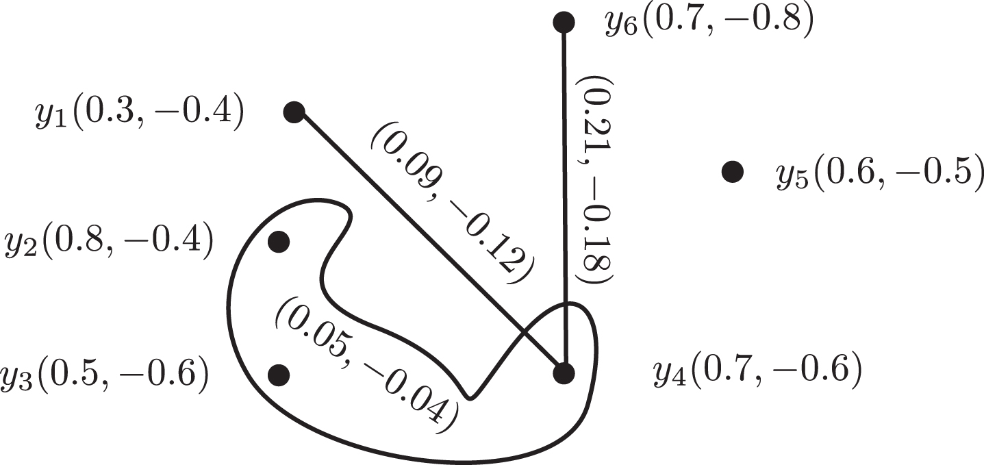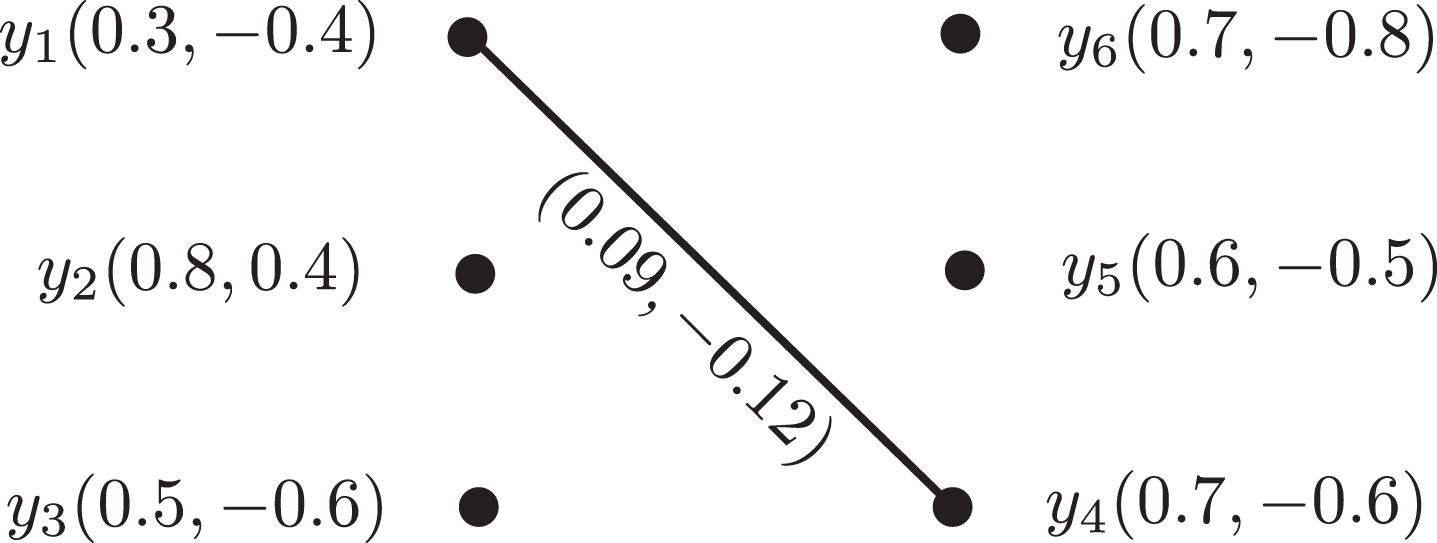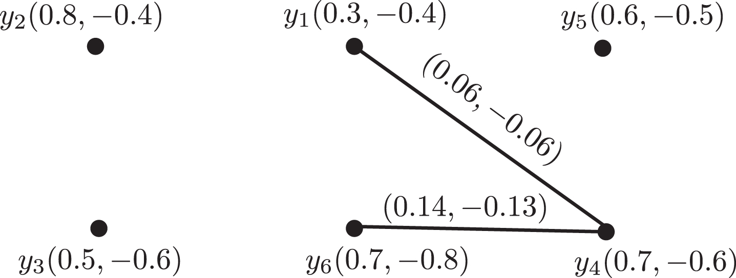The membership grade of the hyperedge E = {y₁, y₂, ⋯ , y_p} is defined as $\begin{matrix} η_{W}^{+} (E) & = & [η_{M}^{+} (y_{1}) \land η_{M}^{+} (y_{2}) \land \dots \land η_{M}^{+} (y_{p})] \times \\ [h (N^{+} (y_{1}) \cap N^{+} (y_{2}) \cap \dots \cap N^{+} (y_{p})) \\ \land h (N^{-} (y_{1}) \cap N^{-} (y_{2}) \cap \dots \cap N^{-} (y_{p}))], \\ η_{W}^{-} (E) & = & [η_{M}^{-} (y_{1}) \lor η_{M}^{-} (y_{2}) \lor \dots \lor η_{M}^{-} (y_{p})] \times \\ [h (N^{+} (y_{1}) \cap N^{+} (y_{2}) \cap \dots \cap N^{+} (y_{p})) \\ \land h (N^{-} (y_{1}) \cap N^{-} (y_{2}) \cap \dots \cap N^{-} (y_{p}))] . \end{matrix}$

Example 3.12. Consider the BF digraph $\vec{J} = (M, \vec{N})$ as given in Figure 3.1. The intersection of the hyperedges of $CH (\vec{J})$ and $CEH (\vec{J})$ are the hyperedges of $DCH (\vec{J})$ . So there is only one hyperedge of $DCH (\vec{J})$ which is {y₁, y₄}. Now we compute the membership grade of this hyperedge. $\begin{matrix} η_{W}^{+} ({y_{1}, y_{4}}) & = & [η_{M}^{+} (y_{1}) \land η_{M}^{+} (y_{4})] \times [h (N^{+} (y_{1}) \\ \cap N^{+} (y_{4})) \land h (N^{-} (y_{1}) \cap N^{-} (y_{4}))] \\ = 0.3 \times 0.3 = 0.09, \\ η_{W}^{-} ({y_{1}, y_{4}}) & = & [η_{M}^{-} (y_{1}) \lor η_{M}^{-} (y_{4})] \times [h (N^{+} (y_{1}) \\ \cap N^{+} (y_{4})) \land h (N^{-} (y_{1}) \cap N^{-} (y_{4}))] \\ = - 0.4 \times 0.3 = - 0.12 . \end{matrix}$

The BF double competition hypergraph is given in Figure 3.7.

Fig. 3.7

$DCH (\vec{J})$

Lemma 3.13. The $DCH (\vec{J})$ is the intersection of $R \circ H (A)$ and $C \circ H (A)$ .

Proof. Let $\vec{J} = (M, \vec{N})$ be a BF digraph on Y. Suppose E = {y₁, y₂, ⋯ , y_p} is any hyperedge of BF double competition hypergraph $DCH (\vec{J})$ = (M, W) .

$\begin{matrix} η_{W}^{+} (E) & = & [η_{M}^{+} (y_{1}) \land η_{M}^{+} (y_{2}) \land \dots \land η_{M}^{+} (y_{p})] \times \\ [h (N^{+} (y_{1}) \cap N^{+} (y_{2}) \cap \dots \cap N^{+} (y_{p})) \\ \land h (N^{-} (y_{1}) \cap N^{-} (y_{2}) \cap \dots \cap N^{-} (y_{p}))], \\ η_{W}^{-} (E) & = & [η_{M}^{-} (y_{1}) \lor η_{M}^{-} (y_{2}) \lor \dots \lor η_{M}^{-} (y_{p})] \times \\ [h (N^{+} (y_{1}) \cap N^{+} (y_{2}) \cap \dots \cap N^{+} (y_{p})) \\ \land h (N^{-} (y_{1}) \cap N^{-} (y_{2}) \cap \dots \cap N^{-} (y_{p}))], \\ \Rightarrow η_{W}^{+} (E) & = & [η_{M}^{+} (y_{1}) \land η_{M}^{+} (y_{2}) \land \dots \land η_{M}^{+} (y_{p})] \\ \times [max_{j} {η_{\vec{N}}^{+} (y_{1} y_{j}) \land η_{\vec{N}}^{+} (y_{2} y_{j}) \land \dots \land \\ η_{\vec{N}}^{+} (y_{p} y_{j})} \land max_{i} {η_{\vec{N}}^{+} (y_{i} y_{1}) \\ \land η_{\vec{N}}^{+} (y_{i} y_{2}) \land \dots \land η_{\vec{N}}^{+} (y_{i} y_{p})}], \\ η_{W}^{-} (E) & = & [η_{M}^{-} (y_{1}) \lor η_{M}^{-} (y_{2}) \lor \dots \lor η_{M}^{-} (y_{p})] \\ \times [max_{j} {η_{\vec{N}}^{+} (y_{1} y_{j}) \land η_{\vec{N}}^{+} (y_{2} y_{j}) \land \dots \\ \land η_{\vec{N}}^{+} (y_{p} y_{j})} \land max_{i} {η_{\vec{N}}^{+} (y_{i} y_{1}) \\ \land η_{\vec{N}}^{+} (y_{i} y_{2}) \land \dots \land η_{\vec{N}}^{+} (y_{i} y_{p})}], \\ \Rightarrow η_{W}^{+} (E) & = & [{η_{M}^{+} (y_{1}) \land η_{M}^{+} (y_{2}) \land \dots \land η_{M}^{+} (y_{p})} \times max_{j} \\ {η_{\vec{N}}^{+} (y_{1} y_{j}) \land η_{\vec{N}}^{+} (y_{2} y_{j}) \land \dots \land η_{\vec{N}}^{+} (y_{p} y_{j})] \\ \land [{η_{M}^{+} (y_{1}) \land η_{M}^{+} (y_{2}) \land \dots \land η_{M}^{+} (y_{p})} \times max_{i} \\ {η_{\vec{N}}^{+} (y_{i} y_{1}) \land η_{\vec{N}}^{+} (y_{i} y_{2}) \land \dots \land η_{\vec{N}}^{+} (y_{i} y_{p})}], \\ η_{W}^{-} (E) & = & [{η_{M}^{-} (y_{1}) \lor η_{M}^{-} (y_{2}) \lor \dots \lor η_{M}^{-} (y_{p})} \times max_{j} \\ {η_{\vec{N}}^{+} (y_{1} y_{j}) \land η_{\vec{N}}^{+} (y_{2} y_{j}) \land \dots \land η_{\vec{N}}^{+} (y_{p} y_{j})] \\ \land [{η_{M}^{-} (y_{1}) \lor η_{M}^{-} (y_{2}) \lor \dots \lor η_{M}^{-} (y_{p})} \times max_{i} \\ {η_{\vec{N}}^{+} (y_{i} y_{1}) η_{\vec{N}}^{+} (y_{i} y_{2}) \land \dots \land η_{\vec{N}}^{+} (y_{i} y_{p})}], \\ \Rightarrow η_{W}^{+} (E) & = & η_{V}^{+} (E) \land η_{X}^{+} (E), \\ η_{W}^{-} (E) & = & η_{V}^{-} (E) \land η_{X}^{-} (E) . \end{matrix}$

Definition 3.14. Let $\vec{J} = (M, \vec{N})$ be a BF digraph on Y . The BF niche hypergraph $N H (\vec{J})$ =(M, B) containing the BF vertex set same as in BF digraph $\vec{J}$ and E = {y₁, y₂, ⋯ , y_p}⊆Y is the hyperedge of $N H (\vec{J})$ if either N ⁺ (y₁)∩ N ⁺ (y₂) ∩ ⋯ ∩ N ⁺ (y_p) ≠ ∅ or N ^- (y₁)∩ N ^- (y₂) ∩ ⋯ ∩ N ^- (y_p) ≠ ∅. The membership grade of the hyperedge E = {y₁, y₂, ⋯ , y_p} is defined as $\begin{matrix} η_{B}^{+} (E) & = & [η_{M}^{+} (y_{1}) \land η_{M}^{+} (y_{2}) \land \dots \land η_{M}^{+} (y_{p})] \times \\ [h (N^{+} (y_{1}) \cap N^{+} (y_{2}) \cap \dots \cap N^{+} (y_{p})) \\ \lor h (N^{-} (y_{1}) \cap N^{-} (y_{2}) \cap \dots \cap N^{-} (y_{p}))], \\ η_{B}^{-} (E) & = & [η_{M}^{-} (y_{1}) \lor η_{M}^{-} (y_{2}) \lor \dots \lor η_{M}^{-} (y_{p})] \times \\ [h (N^{+} (y_{1}) \cap N^{+} (y_{2}) \cap \dots \cap N^{+} (y_{p})) \\ \lor h (N^{-} (y_{1}) \cap N^{-} (y_{2}) \cap \dots \cap N^{-} (y_{p}))] . \end{matrix}$

Example 3.15. Consider the BF digraph $\vec{J} = (M, \vec{N})$ as given in Figure 3.1. The union of the hyperedges of $CH (\vec{J})$ and $CEH (\vec{J})$ are the hyperedges of $NH (\vec{J})$ which are {y₁, y₄} , {y₁, y₃} , {y₁, y₅, y₆} , {y₄, y₆} , and {y₂, y₃, y₄}. For membership grade of these hyperedges see Examples 3.2 and 3.4.

The BF niche hypergraph is given in Figure 3.8.

Fig. 3.8

$NH (\vec{J})$

Lemma 3.16. The $NH (\vec{J})$ is the union of $R \circ H (A)$ and $C \circ H (A)$ .

Remark 3.17. From the above discussion and Figures we can see the following relationships between hypergraphs.

BF double competition hypergraph is the subset of BF competition hypergraph and BF niche hypergraph, and BF competition hypergraph is the subset of BF niche hypergraph. $DCH (\vec{J}) \subseteq CH (\vec{J}) \subseteq NH (\vec{J})$ .

BF double competition hypergraph is the subset of BF common enemy hypergraph and BF niche hypergraph, and BF common enemy hypergraph is the subset of BF niche hypergraph. $DCH (\vec{J}) \subseteq CEH (\vec{J}) \subseteq NH (\vec{J}) .$

Figure 3.9 depicts the relationships among certain types of BF hypergraphs.

Fig. 3.9

Relations among BF hypergraphs

We now discuss an extension of BF competition hypergraphs $CH (\vec{J})$ and BF common enemy hypergraphs $CEH (\vec{J})$ .

Definition 3.18. Let $\vec{J} = (M, \vec{N})$ be a BF digraph on Y and suppose k = (k ⁺, k ^-) , where k ⁺ ∈ [0, 1] and k ^- ∈ [-1, 0]. The BF k -competition hypergraph $C_{k} (\vec{J})$ = (M, O) of a BF digraph $\vec{J}$ containing the BF vertex set same as in BF digraph $\vec{J}$ and E = {y₁, y₂, ⋯ , y_p} ⊆Y is the hyperedge of $C_{k} (\vec{J})$ if $| η_{N^{+} (y_{1}) \cap N^{+} (y_{2}) \cap \dots \cap N^{+} (y_{p})}^{+} |$ > k ⁺ and $| η_{N^{+} (y_{1}) \cap N^{+} (y_{2}) \cap \dots \cap N^{+} (y_{p})}^{-} |$ < k ^- . The membership grade of the hyperedge E = {y₁, y₂, ⋯ , y_p} is defined as

$\begin{matrix} η_{O}^{+} (E) & = & \frac{h^{+} - k^{+}}{h^{+}} [η_{M}^{+} (y_{1}) \land η_{M}^{+} (y_{2}) \land \dots \land η_{M}^{+} (y_{p})] \\ \times h (N^{+} (y_{1}) \cap N^{+} (y_{2}) \cap \dots \cap N^{+} (y_{p})), \\ η_{O}^{-} (E) & = & \frac{h^{-} - k^{-}}{h^{-}} [η_{M}^{-} (y_{1}) \lor η_{M}^{-} (y_{2}) \lor \dots \lor η_{M}^{-} (y_{p})] \\ \times h (N^{+} (y_{1}) \cap N^{+} (y_{2}) \cap \dots \cap N^{+} (y_{p})), \end{matrix}$

where |N ⁺ (y₁) ∩ N ⁺ (y₂) ∩ ⋯ ∩ N ⁺ (y_p) | = (h ⁺, h ^-).

Remark 3.19. At k = 0, the BF k -competition hypergraph $C_{k} (\vec{J})$ is merely BF competition hypergraph $CH (\vec{J})$ . Following given an example of BF (0.1, - 0.1)-competition hypergraph.

Example 3.20. Consider $\vec{J} = (M, \vec{N}$ ) be a BF digraph on Y as shown in Figure 3.1. As E₂ = {y₁, y₃}, E₃ = {y₁, y₄} , and E₄ = {y₁, y₅, y₆} (see Example 3.2). Here $\begin{matrix} N^{+} (y_{1}) \cap N^{+} (y_{3}) & = & {(y_{2}, 0.3, - 0.4)}, \\ | N^{+} (y_{1}) \cap N^{+} (y_{3}) | & = & (h^{+}, h^{-}) = (0.3, - 0.4) . \end{matrix}$ So $| η_{N^{+} (y_{1}) \cap N^{+} (y_{3})}^{+} | = 0.3 > 0.1$ and $| η_{N^{+} (y_{1}) \cap N^{+} (y_{3})}^{-} | = - 0.4 < - 0.1$ and by Definition 3.18, E₂ is the hyperedge of $C_{k} (\vec{J})$ . Now we calculate the membership grade of this hyperedge. $\begin{matrix} η_{O}^{+} (E_{2}) & = & \frac{0.3 - 0.1}{0.3} (η_{M}^{+} (y_{1}) \land η_{M}^{+} (y_{3})) \\ \times h (N^{+} (y_{1}) \cap N^{+} (y_{3})) = 0.06, \\ η_{O}^{-} (E_{2}) & = & \frac{- 0.4 + 0.1}{- 0.4} (η_{M}^{-} (y_{1}) \lor η_{M}^{-} (y_{3})) \\ \times h (N^{+} (y_{1}) \cap N^{+} (y_{3})) = - 0.09 . \end{matrix}$ Similarly, $η_{O}^{+} (E_{3}) = 0.06$ and $η_{O}^{-} (E_{3}) = - 0.09$ . E₄ is not the hyperedge of $C_{k} (\vec{J})$ because $| η_{N^{+} (y_{1}) \cap N^{+} (y_{5}) \cap N^{+} (y_{6})}^{+} | = 0.1 ≯ 0.1$ .

The BF k -competition hypergraph is given in Figure 3.10.

Fig. 3.10

BF (0.1, - 0.1)-competition hypergraph

Definition 3.21. Let $\vec{J} = (M, \vec{N})$ be a BF digraph on Y and suppose k = (k ⁺, k ^-) , where k ⁺ ∈ [0, 1] and k ^- ∈ [-1, 0]. The BF k -common enemy hypergraph $_{C} k E (\vec{J})$ = (M, A) of a BF digarph $\vec{J}$ containing the BF vertex set same as in BF digraph $\vec{J}$ and E = {y₁, y₂, ⋯ , y_p} ⊆Yis the hyperedge of $_{C} k E (\vec{J})$ if $| η_{N^{-} (y_{1}) \cap N^{-} (y_{2}) \cap \dots \cap N^{-} (y_{p})}^{+} |$ > k ⁺ and $| η_{N^{-} (y_{1}) \cap N^{-} (y_{2}) \cap \dots \cap N^{-} (y_{p})}^{-} |$ < k ^- . The membership grade of the hyperedge E = {y₁, y₂, ⋯ , y_p} is defined as

$\begin{matrix} η_{A}^{+} (E) & = & \frac{h^{+} - k^{+}}{h^{+}} [η_{M}^{+} (y_{1}) \land η_{M}^{+} (y_{2}) \land \dots \land η_{M}^{+} (y_{p})] \\ \times h (N^{-} (y_{1}) \cap N^{-} (y_{2}) \cap \dots \cap N^{-} (y_{p})), \\ η_{A}^{-} (E) & = & \frac{h^{-} - k^{-}}{h^{-}} [η_{M}^{-} (y_{1}) \lor η_{M}^{-} (y_{2}) \lor \dots \lor η_{M}^{-} (y_{p})] \\ \times h (N^{-} (y_{1}) \cap N^{-} (y_{2}) \cap \dots \cap N^{-} (y_{p})), \end{matrix}$

where |N ^- (y₁) ∩ N ^- (y₂) ∩ ⋯ ∩ N ^- (y_p) | = (h ⁺, h ^-).

Remark 3.22. At k = 0, the BF k -common enemy hypergraph $_{C} k E (\vec{J})$ is merely BF common enemy hypergraph $CEH (\vec{J})$ . Following given an example of BF (0.1, - 0.1)-common-enemy hypergraph.

Example 3.23. Consider the BF digraph $\vec{J} = (M, \vec{N}$ ) on Y as given in Figure 3.1. As E₅ = {y₄, y₆}, E₆ = {y₁, y₄} , and E₄ = {y₂, y₃, y₄} (see Example 3.4). Here $\begin{matrix} N^{-} (y_{4}) \cap N^{-} (y_{6}) & = & {(y_{5}, 0.3, - 0.4)}, \\ | N^{-} (y_{4}) \cap N^{-} (y_{6}) | & = & (h^{+}, h^{-}) = (0.3, - 0.4) . \end{matrix}$ So $| η_{N^{-} (y_{4}) \cap N^{-} (y_{6})}^{+} | = 0.3 > 0.1$ and $| η_{N^{-} (y_{4}) \cap N^{-} (y_{6})}^{-} | = - 0.4 < - 0.1$ and by Definition 3.21, E₅ is the hyperedge of $_{C} k E (\vec{J})$ . Now we calculate the grade of membership of this hyperedge. $\begin{matrix} η_{A}^{+} (E_{5}) & = & \frac{0.3 - 0.1}{0.3} (η_{M}^{+} (y_{4}) \land η_{M}^{+} (y_{6})) \\ \times h (N^{-} (y_{4}) \cap N^{-} (y_{6})) = 0.14, \\ η_{A}^{-} (E_{5}) & = & \frac{- 0.4 + 0.1}{- 0.4} (η_{M}^{-} (y_{4}) \lor η_{M}^{-} (y_{6})) \\ \times h (N^{-} (y_{4}) \cap N^{-} (y_{6})) = - 0.13 . \end{matrix}$ Similarly, $η_{A}^{+} (E_{6}) = 0.06$ and $η_{A}^{-} (E_{6}) = - 0.06$ . The BF k -common enemy hypergraph is given in Figure 3.11.

Fig. 3.11

BF (0.1, - 0.1)-common enemy hypergraph

Definition 3.24. Let H = (M, R) be a BF hypergraph on Y . A hyperedge E_i={y₁, y₂, ⋯ , y_p} ⊆ Y is called strong if $η_{R}^{+} (E_{i}) \geq \frac{1}{2} ⋀_{k = 1}^{p} η_{M_{i}}^{+} (y_{k})$ and $η_{R}^{-} (E_{i}) \leq \frac{1}{2} ⋁_{k = 1}^{p} η_{M_{i}}^{-} (y_{k})$ .

Theorem 3.25. Let $\vec{J} = (M, \vec{N})$ be a BF digraph on Y . If N⁺ (y₁) ∩ N⁺ (y₂) ∩ ⋯ ∩ N⁺ (y_p) contains only one vertex then the hyperedge E={y₁, y₂, ⋯ , y_p} of $CH (\vec{J})$ is strong iff $| η_{N^{+} (y_{1}) \cap N^{+} (y_{2}) \cap \dots \cap N^{+} (y_{p})}^{+} |$ > $\frac{1}{2}$ and $| η_{N^{+} (y_{1}) \cap N^{+} (y_{2}) \cap \dots \cap N^{+} (y_{p})}^{-} |$ < $\frac{1}{2}$ .

Proof. Let N ⁺ (y₁) ∩ N ⁺ (y₂) ∩ ⋯ ∩ N ⁺ (y_p) = {a, m ⁺, m ^-} , where m ⁺ and m ^- are membership values of a. Thus, |N ⁺ (y₁) ∩ N ⁺ (y₂) ∩ ⋯ ∩ N ⁺ (y_p) | = {m ⁺, m ^-} , where $m^{+} = | η_{N^{+} (y_{1}) \cap N^{+} (y_{2}) \cap \dots \cap N^{+} (y_{p})}^{+} |$ and $m^{-} = | η_{N^{+} (y_{1}) \cap N^{+} (y_{2}) \cap \dots \cap N^{+} (y_{p})}^{-} |$ . Since h (N ⁺ (y₁) ∩ N ⁺ (y₂) ∩ ⋯ ∩ N ⁺ (y_p)) = m ⁺ and $CH (\vec{J})$ = (M, R). So $\begin{matrix} η_{R}^{+} (E) & = & m^{+} \times [η_{M}^{+} (y_{1}) \land η_{M}^{+} (y_{2}) \land \dots \land η_{M}^{+} (y_{p})], \\ η_{R}^{-} (E) & = & m^{+} \times [η_{M}^{-} (y_{1}) \lor η_{M}^{-} (y_{2}) \lor \dots \lor η_{M}^{-} (y_{p})] . \end{matrix}$ Hence the hyperedge E = {y₁, y₂, ⋯ , y_p} in $CH (\vec{J})$ is strong iff m ⁺ > 0.5 and m ^- < 0.5.

Theorem 3.26. Let $\vec{J} = (M, \vec{N})$ be a BF digraph on Y . If N^- (y₁) ∩ N^- (y₂) ∩ ⋯ ∩ N^- (y_p) contains only one vertex then the hyperedge E={y₁, y₂, ⋯ , y_p} of $CEH (\vec{J})$ is strong iff $| η_{N^{-} (y_{1}) \cap N^{-} (y_{2}) \cap \dots \cap N^{-} (y_{p})}^{+} |$ > $\frac{1}{2}$ and $| η_{N^{-} (y_{1}) \cap N^{-} (y_{2}) \cap \dots \cap N^{-} (y_{p})}^{-} |$ < $\frac{1}{2}$ .

Theorem 3.27. Let $\vec{J} = (M, \vec{N})$ be a BF digraph on a non-void set Y . If h (N⁺ (y₁) ∩ N⁺ (y₂) ∩ ⋯ N⁺ (y_p)) =1, $| η_{N^{+} (y_{1}) \cap N^{+} (y_{2}) \cap \dots N^{+} (y_{p})}^{+} |$ > 2k⁺, and $| η_{N^{+} (y_{1}) \cap N^{+} (y_{2}) \cap \dots N^{+} (y_{p})}^{-} |$ < 2k^- for some y₁, y₂, ⋯ , y_p ∈ Y then the hyperedge E = {y₁, y₂, ⋯ , y_p} is strong in $C_{k} (\vec{J})$ .

Proof. Let $C_{k} (\vec{J})$ = (M, O) be a BF k-competition hypergraph corresponding to the $\vec{J} = (M, \vec{N})$ . Let h (N ⁺ (y₁) ∩ N ⁺ (y₂) ∩ ⋯ N ⁺ (y_p)) =1, $| η_{N^{+} (y_{1}) \cap N^{+} (y_{2}) \cap \dots N^{+} (y_{p})}^{+} |$ >2k ⁺, and $| η_{N^{+} (y_{1}) \cap N^{+} (y_{2}) \cap \dots N^{+} (y_{p})}^{-} |$ <2k ^- . Suppose E = {y₁, y₂, ⋯ , y_p} is any hyperedge of $C_{k} (\vec{J})$ and |N ⁺ (y₁) ∩ N ⁺ (y₂) ∩ ⋯ N ⁺ (y_p) |= (h ⁺, h ^-). Now

Since h (N ⁺ (y₁) ∩ N ⁺ (y₂) ∩ ⋯ N ⁺ (y_p)) =1 .

$\begin{matrix} η_{O}^{+} (E) & = & \frac{h^{+} - k^{+}}{h^{+}} (η_{M}^{+} (y_{1}) \land η_{M}^{+} (y_{2}) \land \dots \land η_{M}^{+} (y_{p})), \\ η_{O}^{-} (E) & = & \frac{h^{-} - k^{-}}{h^{-}} (η_{M}^{-} (y_{1}) \lor η_{M}^{-} (y_{2}) \lor \dots \lor η_{M}^{-} (y_{p})), \\ η_{O}^{+} (E) & > & \frac{1}{2} (η_{M}^{+} (y_{1}) \land η_{M}^{+} (y_{2}) \land \dots \land η_{M}^{+} (y_{p})), \\ η_{O}^{-} (E) & < & \frac{1}{2} (η_{M}^{-} (y_{1}) \lor η_{M}^{-} (y_{2}) \lor \dots \lor η_{M}^{-} (y_{p})) . \end{matrix}$

Hence the hyperedge E of $C_{k} (\vec{J})$ is strong.

Theorem 3.28. Let $\vec{J} = (M, \vec{N})$ be a BF digraph on a non-void set Y . If h (N^- (y₁) ∩ N^- (y₂) ∩ ⋯ N^- (y_p)) =1, $| η_{N^{-} (y_{1}) \cap N^{-} (y_{2}) \cap \dots N^{-} (y_{p})}^{+} |$ >2k⁺, and $| η_{N^{-} (y_{1}) \cap N^{-} (y_{2}) \cap \dots N^{-} (y_{p})}^{-} |$ <2k^- for some y₁, y₂, ⋯ , y_p ∈ Y then the hyperedge E = {y₁, y₂, ⋯ , y_p} is strong in $C_{k} E (\vec{J}) .$

4 Bipolar fuzzy neighborhood hypergraphs

Now we define the notions of BF open neighborhood hypergraphs, BF closed neighborhood hypergraphs, BF (k)-competition hypergraphs and BF [k]-competition hypergraphs.

Definition 4.1. Let $J = (M, N)$ be a BF graph on a non-empty Z. The BF open-neighborhood hypergraph $N (J) = (M, P)$ of $J$ containing the BF vertex set same as in BF graph $J$ and E = {z₁, z₂, ⋯ , z_p} ⊆Z is the hyperedge of $N (J)$ if N (z₁)∩ N (z₂) ∩ ⋯ ∩ N (z_p) ≠ ∅. The grade of membership of the hyperedge E = {z₁, z₂, ⋯ , z_p} is defined as $\begin{matrix} η_{P}^{+} (E) & = & [η_{M}^{+} (z_{1}) \land η_{M}^{+} (z_{2}) \land \dots \land η_{M}^{+} (z_{p})] \\ \times h (N (z_{1}) \cap N (z_{2}) \cap \dots \cap N (z_{p})), \\ η_{P}^{-} (E) & = & [η_{M}^{-} (z_{1}) \lor η_{M}^{-} (z_{2}) \lor \dots \lor η_{M}^{-} (z_{p})] \\ \times h (N (z_{1}) \cap N (z_{2}) \cap \dots \cap N (z_{p})) . \end{matrix}$

The procedure is given in Algorithm 4.1 for computing BF open neighborhood hypergraph $N (J)$ of a BF graph $J$ .

Algorithm 4.1. Method for construction of BF open neighborhood hypergraph

Compute the BF open neighborhood of each vertex in BF graph $J = (M, N)$ .

Define a relationship f : Z ⟶ Z by f (z_i)=z_j if z_j ∈ supp (N (z_i)).

Determine the category of sets X = {E_i = f^-1 (z_i) : |f^-1 (z_i) |≥2, z_i ∈ Z}, where E_i = {z_i
₁, z_i
₂, ⋯ , z_{i
_r}} is a hyperedge of $N (J)$ .

Compute the grade of membership of each hyperedge by using Definition 4.1.

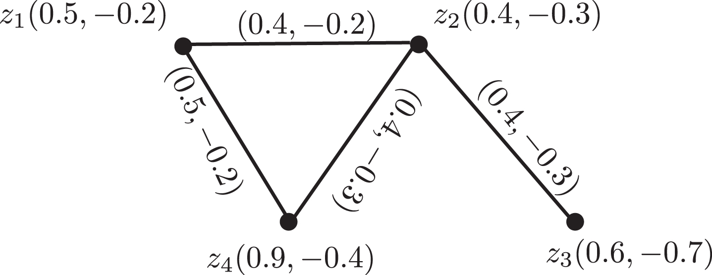
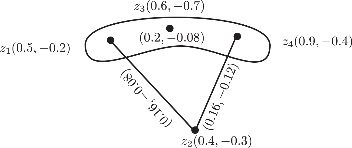
Example 4.2. Consider the BF graph $J = (M, N)$ on Z = {z₁, z₂, z₃, z₄} as shown in Figure 4.1.

Fig. 4.1

BF graph $J$

The BF open neighborhood of each vertex in $J$ is specified in Table 8.

Table 8

BF open neighborhood of vertices in $J$

z ∈ Z	N (z)
z ₁	{(z₂, 0.4, - 0.2) , (z₄, 0.5, - 0.2)}
z ₂	{(z₁, 0.4, - 0.2) , (z₃, 0.4, - 0.3) , (z₄, 0.4, - 0.3)}
z ₃	{(z₂, 0.4, - 0.3)}
z ₄	{(z₁, 0.5, - 0.2) , (z₂, 0.4, - 0.3)}

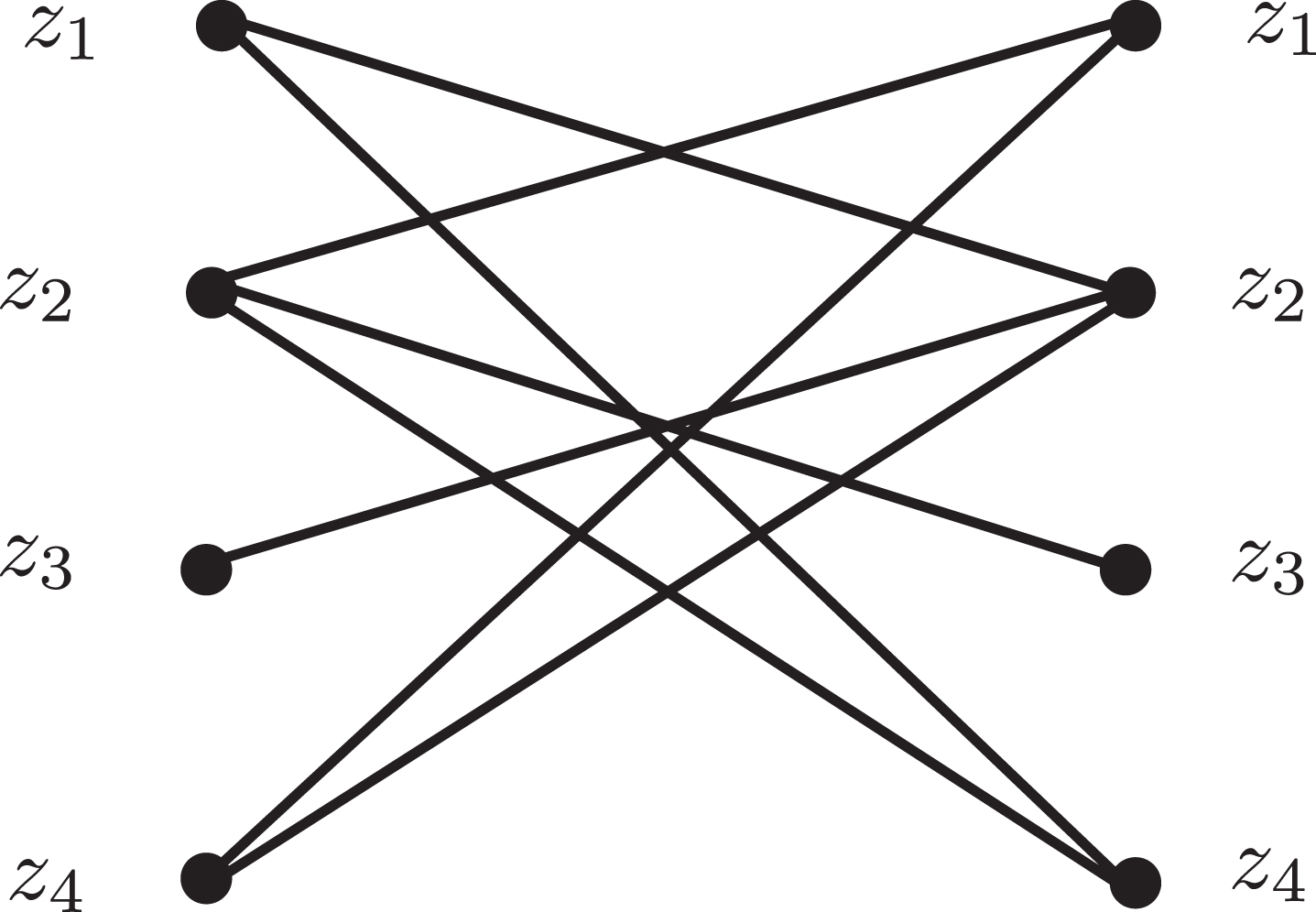
Using Algorithm 4.1, the relationship f : Z ⟶ Z is given in Figure 4.2.

Fig. 4.2

Representation of BF relation in $J$

By using relation 4.2, there are three hyperedges f ^-1 (z₁) = E₁ = {z₂, z₄}, f ^-1 (z₂) = E₂ = {z₁, z₃, z₄} and f ^-1 (z₄) = E₄ = {z₁, z₂} of $N (J)$ . Now we calculate the membership grade of each hyperedge of $N (J)$ . $\begin{matrix} η_{P}^{+} (E_{2}) & = & [η_{M}^{+} (z_{1}) \land η_{M}^{+} (z_{3}) \land η_{M}^{+} (z_{4})] \\ \times h (N (z_{1}) \cap N (z_{3}) \cap N (z_{4})) \\ = 0.5 \times 0.4 = 0.2, \\ η_{P}^{-} (E_{2}) & = & [η_{M}^{-} (z_{1}) \lor η_{M}^{-} (z_{3}) \lor η_{M}^{-} (z_{4})] \\ \times h (N (z_{1}) \cap N (z_{3}) \cap N (z_{4})) \\ = - 0.2 \times 0.4 = - 0.08 . \end{matrix}$ Similarly, $η_{P}^{+} (E_{4}) = 0.16$ and $η_{P}^{-} (E_{4}) = - 0.08$ , $η_{P}^{+} (E_{1}) = 0.16$ and $η_{P}^{-} (E_{1}) = - 0.12$ .

The BF open neighborhood hypergraph is given in Figure 4.3.

Fig. 4.3

$N (J)$

Definition 4.3. Let $J = (M, N)$ be a BF graph on Z. The BF closed-neighborhood hypergraph $N = (M, T)$ on Z containing the BF vertex set same as in BF graph $J$ and E = {z₁, z₂, ⋯ , z_p} is the hyperedge of $N [J]$ if N [z₁]∩ N [z₂] ∩ ⋯ ∩ N [z_p] ≠ ∅. The membership grade of the hyperedge E = {z₁, z₂, ⋯ , z_p} is defined as $\begin{matrix} η_{T}^{+} (E) & = & [η_{M}^{+} (z_{1}) \land η_{M}^{+} (z_{2}) \land \dots \land η_{M}^{+} (z_{p})] \\ \times h (N [z_{1}] \cap N [z_{2}] \cap \dots \cap N [z_{p}]), \\ η_{T}^{-} (E) & = & [η_{M}^{-} (z_{1}) \lor η_{M}^{-} (z_{2}) \lor \dots \lor η_{M}^{-} (z_{p})] \\ \times h (N [z_{1}] \cap N [z_{2}] \cap \dots \cap N [z_{p}]) . \end{matrix}$

Definition 4.4. Let $J = (M, N)$ be a BF graph on Z and k = (k ⁺, k ^-) where, k ⁺ ∈ [0, 1] and k ^- ∈ [-1, 0]. The BF (k)-competition hypergraph $_{N} k (J)$ = (M, D) of $J$ containing the BF vertex set same as in BF graph $J$ and E = {y₁, y₂, ⋯ , y_p} ⊆Z is the hyperedge of $_{N} k (J)$ if $| η_{N (y_{1}) \cap N (y_{2}) \cap \dots \cap N (y_{p})}^{+} | > k^{+}$ and $| η_{N (y_{1}) \cap N (y_{2}) \cap \dots \cap N (y_{p})}^{-} | < k^{-} .$ The membership grade of the hyperedge E = {y₁, y₂, ⋯ , y_p} is defined as $\begin{matrix} η_{D}^{+} (E) & = & \frac{h^{+} - k^{+}}{h^{+}} [η_{M}^{+} (y_{1}) \land η_{M}^{+} (y_{2}) \land \dots \land η_{M}^{+} \\ (y_{p})] \times h (N (y_{1}) \cap N (y_{2}) \cap \dots \cap N (y_{p})), \\ η_{D}^{-} (E) & = & \frac{h^{-} - k^{-}}{h^{-}} [η_{M}^{-} (y_{1}) \lor η_{M}^{-} (y_{2}) \lor \dots \lor η_{M}^{-} \\ (y_{p})] \times h (N (y_{1}) \cap N (y_{2}) \cap \dots \cap N (y_{p})), \end{matrix}$

where |N (y₁) ∩ N (y₂) ∩ ⋯ ∩ N (y_p) | = (h ⁺, h ^-).

Definition 4.5. Let $J = (M, N)$ be a BF graph on Z and k = (k ⁺, k ^-) where, k ⁺ ∈ [0, 1] and k ^- ∈ [-1, 0]. The BF [k]-competition hypergraph $_{N} k [J]$ = (M, C) of $J$ containing the BF vertex set same as in BF graph $J$ and E = {y₁, y₂, ⋯ , y_p} ⊆Z is the hyperedge of $_{N} k [J]$ if $| η_{N [y_{1}] \cap N [y_{2}] \cap \dots \cap N [y_{p}]}^{+} |$ >k ⁺ and $| η_{N [y_{1}] \cap N [y_{2}] \cap \dots \cap N [y_{p}]}^{-} |$ <k ^- . The membership grade of the hyperedge E = {y₁, y₂, ⋯ , y_p} is defined as $\begin{matrix} η_{C}^{+} (E) & = & \frac{h^{+} - k^{+}}{h^{+}} [η_{M}^{+} (y_{1}) \land η_{M}^{+} (y_{2}) \land \dots \land η_{M}^{+} \\ (y_{p})] \times h (N [y_{1}] \cap N [y_{2}] \cap \dots \cap N [y_{p}]), \\ η_{C}^{-} (E) & = & \frac{h^{-} - k^{-}}{h^{-}} [η_{M}^{-} (y_{1}) \lor η_{M}^{-} (y_{2}) \lor \dots \lor η_{M}^{-} \\ (y_{p})] \times h (N [y_{1}] \cap N [y_{2}] \cap \dots \cap N [y_{p}]), \end{matrix}$ where |N [y₁] ∩ N [y₂] ∩ ⋯ ∩ N [y_p] | = (h ⁺, h ^-).

Remark 4.6. At k = 0, both BF (k)-competition hypergraph and BF [k]-competition hypergraph are BF open-neighborhood hypergraph and BF closed-neighborhood hypergraph, respectively.

The relations between BF neighborhood hypergraphs and BF k -competition hypergraphs are given in the following theorems.

Theorem 4.7. Let $\vec{J} = (M, \vec{N})$ be a symmetric BF digraph on Y without any loops then $C_{k} (\vec{J})$ = $N_{k} (U (\vec{J}))$ .

Proof Let $U (\vec{J}) = (M, N)$ be an underlying BF graph of a symmetric BF digraph $\vec{J} = (M, \vec{N})$ . Let $N_{k} (U (\vec{J})) = (M, D)$ and $C_{k} (\vec{J}) = (M, O)$ . The $C_{k} (\vec{J})$ and the underlying BF graph $U (\vec{J})$ have the same vertex set as in $\vec{J .}$ Hence $N_{k} (U (\vec{J}))$ has the same vertex set as in $\vec{J .}$ Now we want to show that O ({y₁, y₂, ⋯ , y_p}) = D ({y₁, y₂, ⋯ , y_p}) for every y₁, y₂, ⋯ , y_p ∈ Y .

Case 1: If $O ({y_{1}, y_{2}, \dots, y_{p}}) = (η_{O}^{+} ({y_{1}, y_{2}, \dots, y_{p}}), η_{O}^{-} ({y_{1}, y_{2}, \dots, y_{p}})) = (0, 0)$ in $C_{k} (\vec{J})$ then either $| η_{N^{+} (y_{1}) \cap N^{+} (y_{2}) \cap \dots \cap N^{+} (y_{p})}^{+} | ≯ k^{+}$ or $| η_{N^{+} (y_{1}) \cap N^{+} (y_{2}) \cap \dots \cap N^{+} (y_{p})}^{-} | ≮ k^{-}$ Since $\vec{J}$ is a symmetric BF digraph, either $| η_{N (y_{1}) \cap N (y_{2}) \cap \dots \cap N (y_{p})}^{+} | ≯ k^{+}$ or $| η_{N (y_{1}) \cap N (y_{2}) \cap \dots \cap N (y_{p})}^{-} | ≮ k^{-}$ in $U (\vec{J})$ . Consequently, $D ({y_{1}, y_{2}, \dots, y_{p}}) = (η_{D}^{+} ({y_{1}, y_{2}, \dots, y_{p}}), η_{D}^{-} ({y_{1}, y_{2}, \dots, y_{p}})) = (0, 0)$ .

Case 2: If O ({y₁, y₂, ⋯ , y_p}) = $(η_{O}^{+} ({y_{1}, y_{2}, \dots, y_{p}}), η_{O}^{-} ({y_{1}, y_{2}, \dots, y_{p}})) \neq (0, 0)$ in BF k-competition hypergraph $C_{k} (\vec{J})$ then $| η_{N^{+} (y_{1}) \cap N^{+} (y_{2}) \cap \dots \cap N^{+} (y_{p})}^{+} | > k^{+}$ and $| η_{N^{+} (y_{1}) \cap N^{+} (y_{2}) \cap \dots \cap N^{+} (y_{p})}^{-} | < k^{-} .$ Since $\vec{J}$ is symmetric BF digraph, h (N (y₁) ∩ N (y₂) ∩ ⋯ ∩ N (y_p)) = h (N ⁺ (y₁) ∩ N ⁺ (y₂) ∩ ⋯ ∩ N ⁺ (y_p)). So $\begin{matrix} η_{O}^{+} ({y_{1}, y_{2}, \dots, y_{p}}) \\ = \frac{h^{+} - k^{+}}{h^{+}} (η_{M}^{+} (y_{1}) \land η_{M}^{+} (y_{2}) \land \dots \land η_{M}^{+} (y_{P})) \\ \times h (N^{+} (y_{1}) \cap N^{+} (y_{2}) \cap \dots \cap N^{+} (y_{p})) \\ = η_{D}^{+} ({y_{1}, y_{2}, \dots, y_{p}}), \\ η_{O}^{-} ({y_{1}, y_{2}, \dots, y_{p}}) \\ = \frac{h^{-} - k^{+}}{h^{-}} (η_{M}^{-} (y_{1}) \lor η_{M}^{-} (y_{2}) \lor \dots \lor η_{M}^{-} (y_{P})) \\ \times h (N^{+} (y_{1}) \cap N^{+} (y_{2}) \cap \dots \cap N^{+} (y_{p})) \\ = η_{D}^{-} ({y_{1}, y_{2}, \dots, y_{p}}) . \end{matrix}$ Hence O ({y₁, y₂, ⋯ , y_p}) = D ({y₁, y₂, ⋯ , y_p}) for all y₁, y₂, ⋯ , y_p.

Theorem 4.8. Let $\vec{J} = (M, \vec{N})$ be a symmetric BF digraph having loops at every vertex then $C_{k} (\vec{J})$ = $N_{k} [U (\vec{J})]$ . Proof. Let $U (\vec{J}) = (M, N)$ be an underlying BF graph of $\vec{J} = (M, \vec{N}) .$ Also, let $N_{k} [U (\vec{J})] = (M, C)$ and $C_{k} (\vec{J}) = (M, O) .$ The $C_{k} (\vec{J})$ and the underlying BF graph $U (\vec{J})$ have the same vertex set as in $\vec{J .}$ Hence $N_{k} [U (\vec{J})]$ has the same vertex set as in $\vec{J .}$ Now we want to show that O ({y₁, y₂, ⋯ , y_p}) = C ({y₁, y₂, ⋯ , y_p}) for every y₁, y₂, ⋯ , y_p ∈ Y . As the $\vec{J}$ has a loop at every vertex so the BF out neighborhood contains the vertex itself.

Case 1: If $O ({y_{1}, y_{2}, \dots, y_{p}}) = (η_{O}^{+} ({y_{1}, y_{2}, \dots, y_{p}}), η_{O}^{-} ({y_{1}, y_{2}, \dots, y_{p}})) = (0, 0)$ in $C_{k} (\vec{J})$ then either $| η_{N^{+} (y_{1}) \cap N^{+} (y_{2}) \cap \dots \cap N^{+} (y_{p})}^{+} | ≯ k^{+}$ or $| η_{N^{+} (y_{1}) \cap N^{+} (y_{2}) \cap \dots \cap N^{+} (y_{p})}^{-} | ≮ k^{-} .$ Since $\vec{J}$ is a symmetric BF digraph, either $| η_{N [y_{1}] \cap N [y_{2}] \cap \dots \cap N [y_{p}]}^{+} | ≯ k^{+}$ or $| η_{N [y_{1}] \cap N [y_{2}] \cap \dots \cap N [y_{p}]}^{-} | ≮ k^{-}$ in $U (\vec{J}) .$ Consequently, $C ({y_{1}, y_{2}, \dots, y_{p}}) = (η_{C}^{+} ({y_{1}, y_{2}, \dots, y_{p}}), η_{C}^{-} ({y_{1}, y_{2}, \dots, y_{p}})) = (0, 0) .$

Case 2: If $O ({y_{1}, y_{2}, \dots, y_{p}}) = (η_{O}^{+} ({y_{1}, y_{2}, \dots, y_{p}}), η_{O}^{-} ({y_{1}, y_{2}, \dots, y_{p}})) \neq (0, 0)$ in BF k-competition hypergraph $C_{k} (\vec{J})$ then $| η_{N^{+} (y_{1}) \cap N^{+} (y_{2}) \cap \dots \cap N^{+} (y_{p})}^{+} | > k^{+}$ and $| η_{N^{+} (y_{1}) \cap N^{+} (y_{2}) \cap \dots \cap N^{+} (y_{p})}^{-} | < k^{-} .$ Since $\vec{J}$ is symmetric BF digraph with loops, |N [y₁] ∩ N [y₂] ∩ ⋯ ∩ N [y_p] | = |N ⁺ (y₁) ∩ N ⁺ (y₂) ∩ ⋯ ∩ N ⁺ (y_p) | and h (N [y₁] ∩ N [y₂] ∩ ⋯ ∩ N [y_p]) = h (N ⁺ (y₁) ∩ N ⁺ (y₂) ∩ ⋯ ∩ N ⁺ (y_p)) . So $\begin{matrix} η_{O}^{+} ({y_{1}, y_{2}, \dots, y_{p}}) \\ = \frac{h^{+} - k^{+}}{h^{+}} (η_{M}^{+} (y_{1}) \land η_{M}^{+} (y_{2}) \land \dots \land η_{M}^{+} (y_{P})) \\ \times h (N^{+} (y_{1}) \cap N^{+} (y_{2}) \cap \dots \cap N^{+} (y_{p})) \\ = η_{C}^{+} ({y_{1}, y_{2} \dots y_{p}}), \\ η_{O}^{-} ({y_{1}, y_{2}, \dots, y_{p}}) \\ = \frac{h^{-} - k^{+}}{h^{-}} (η_{M}^{-} (y_{1}) \lor η_{M}^{-} (y_{2}) \lor \dots \lor η_{M}^{-} (y_{P})) \\ \times h (N^{+} (y_{1}) \cap N^{+} (y_{2}) \cap \dots \cap N^{+} (y_{p})) \\ = η_{C}^{-} ({y_{1}, y_{2}, \dots, y_{p}}) . \end{matrix}$ Hence O ({y₁, y₂, ⋯ , y_p}) = C ({y₁, y₂, ⋯ , y_p}) for all y₁, y₂, ⋯ , y_p .

5 Application of bipolar fuzzy competition hypergraphs

Business competition is the contest or conflict among business rivals that are competing in the same domain. There are multiples companies/brands which sell the same products to trades and various companies. In this competitive domain, every company makes an effort to captivate client attention to its products. Hypergraph theory is a fundamental technique to study the competition between buyer and seller using the structure of hypergraphs. But in all this theory, it is estimated that the nodes and edges of the graphs are explicitly defined. But in real life, these formations cannot be defined explicitly. For instance, companies are distinct according to annual advantages and disadvantages. So to solve these types of bipolar fuzziness problems (advantages and disadvantages are bipolar facts) we need the theory of BF competition hypergraphs.

We now discuss an example application of BF competition hypergraphs in the business market and study how to apply the notion of BF competition hypergraphs in the business market. A technique is given in Algorithm 5.1 which indicates the competitive significance of each company inside the business market.

Algorithm 5.1. Method to calculate the strength of competition in business trade

Input the BF set $M = (η_{M}^{+}, η_{M}^{-})$ of n companies y₁, y₂, ⋯ , y_n.

Define a BF relation $\vec{N}$ = $(η_{\vec{N}}^{+}, η_{\vec{N}}^{-})$ in n companies y₁, y₂, ⋯ , y_n.

Calculate the BF out neighborhood of each company.

Calculate the BF competition hypergraph $CH (\vec{J}) = (M, R)$ by using Algorithm 3.1, where $\vec{J}$ is a BF digraph of n companies.

Evaluate the degree of all vertex y_i as $\begin{matrix} (\deg^{+} (y_{i}), \deg^{-} (y_{i})) & = & \sum_{y_{i} \in E} (η_{R}^{+} (E), η_{R}^{-} (E)), \end{matrix}$ where E is a hyperedge of BF competition hypergraph.

Using the following formula to compute the strength of competition of all companies: $S (y_{i}) = \frac{\deg^{+} (y_{i}) + 1 + \deg^{-} (y_{i})}{2}$ , where 1 ≤ i ≤ n.

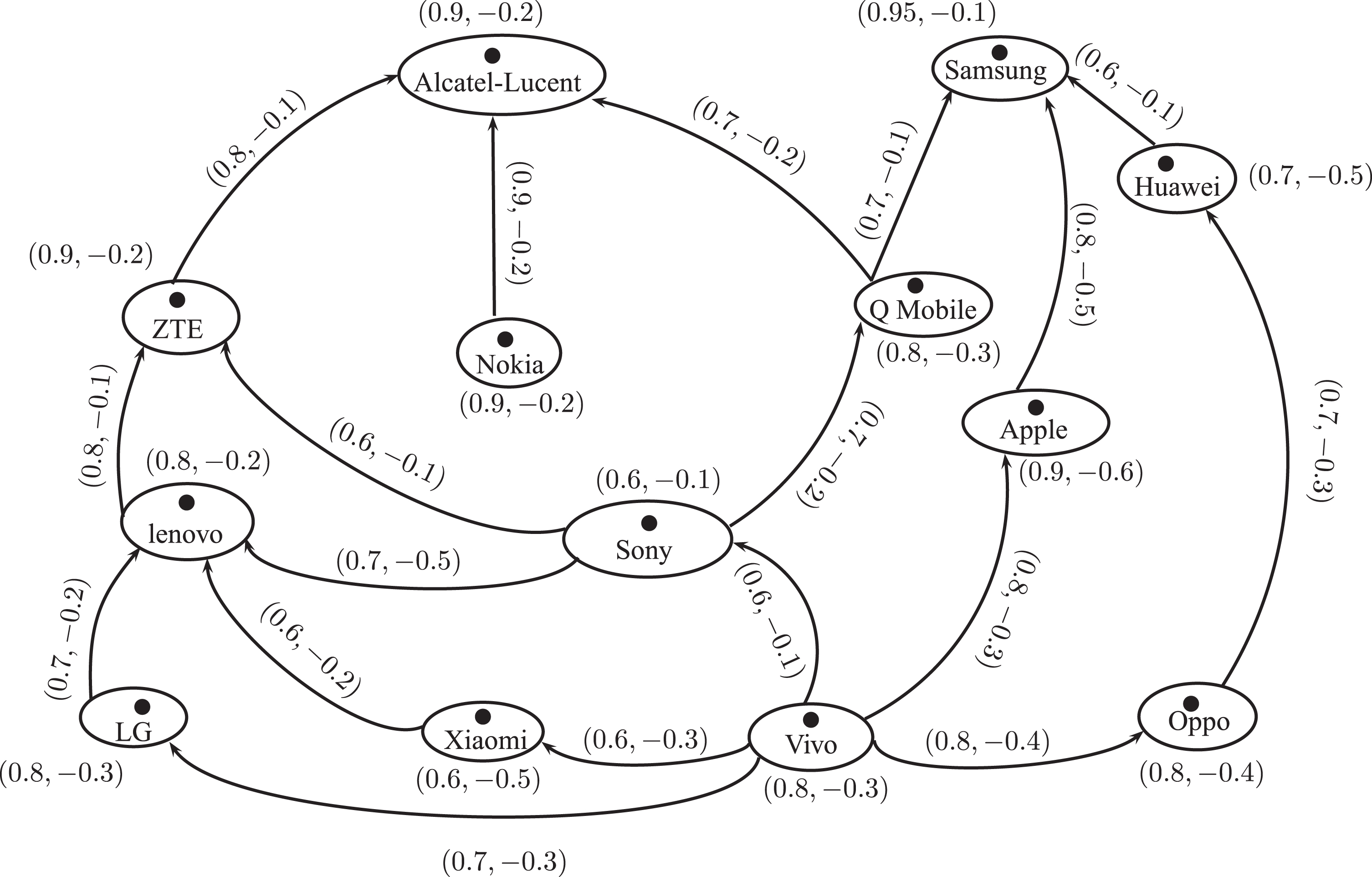
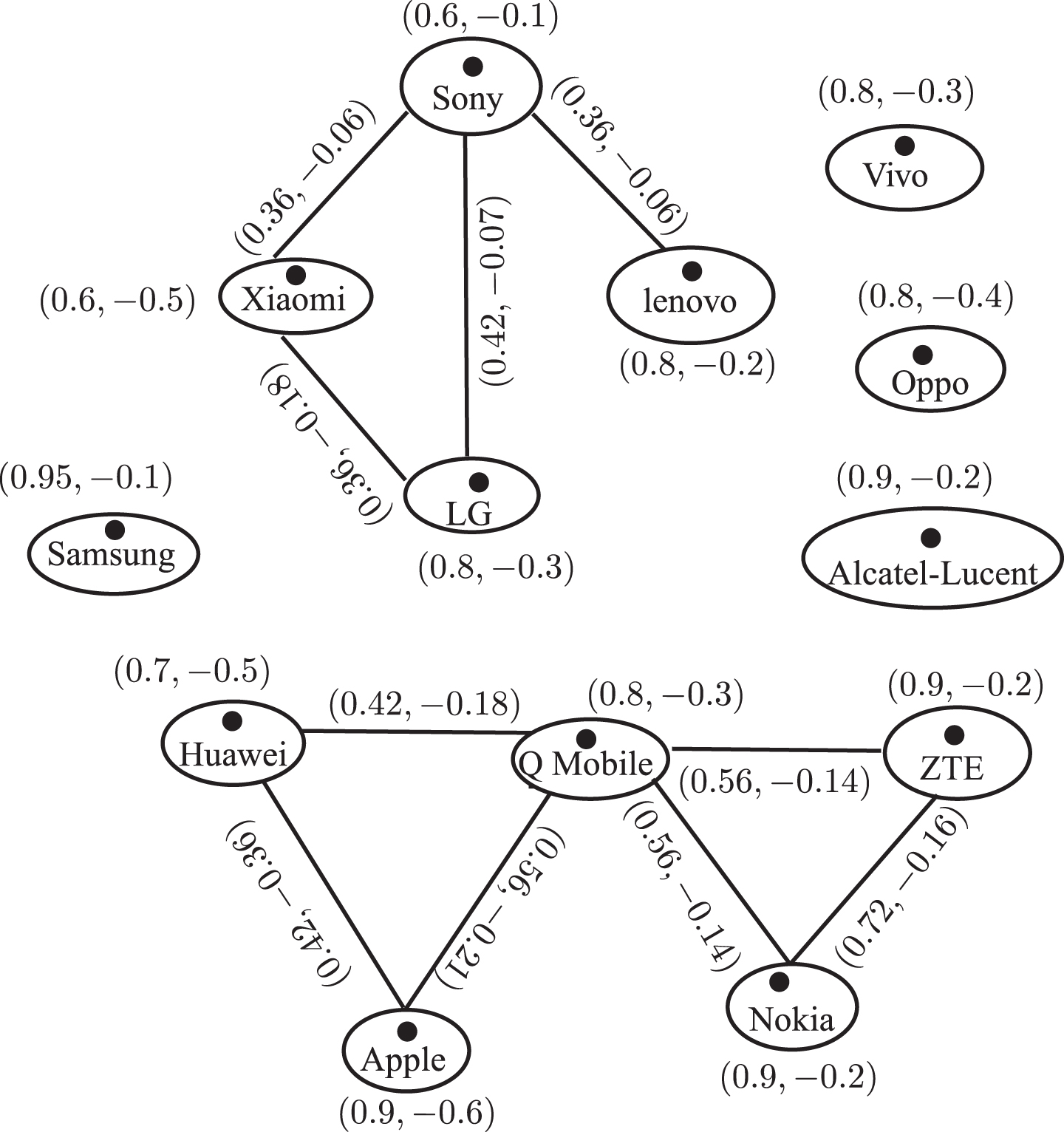
Consider the top 13 world largest mobile companies Samsung, Apple, Huawei, Nokia, Oppo, Q Mobile, LG, Vivo, Xiaomi, Lenovo, ZTE, Alcatel-Lucent, and Sony. Suppose y₁, y₂, ⋯ , y_n indicates the n mobile companies. Consider $\begin{matrix} M & = & {(y_{1} = Samsung, 0.95, - 0.1), (y_{2} = Apple, \\ 0.9, 0.6), (y_{3} = Huawei, 0.7, - 0.5), (y_{4} = \\ Nokia, 0.9, 0.2), (y_{5} = Oppo, 0.8, - 0.4), \\ (y_{6} = QMobile, 0.8, - 0.3), (y_{7} = LG, 0.8, \\ - 0.3), (y_{8} = Vivo, 0.8, - 0.3), (y_{9} = Xiaomi, \\ 0.6, - 0.5), (y_{10} = Levono, 0.8, - 0.2), (y_{11} \\ = ZTE, 0.9, - 0.2), (y_{12} = Alcatel - Lucent, \\ 0.9, - 0.2), (y_{13} = Sony, 0.6, - 0.1)}, \\ \vec{N} & = & {(\vec{y_{2} y_{1}}, 0.8, - 0.5), (\vec{y_{3} y_{1}}, 0.6, - 0.1), (\vec{y_{4} y_{12}}, \\ 0.9, - 0.2), (\vec{y_{5} y_{3}}, 0.7, - 0.3), (\vec{y_{6} y_{1}}, 0.7, \\ - 0.1), (\vec{y_{8} y_{5}}, 0.8, - 0.4), (\vec{y_{8} y_{2}}, 0.8, - 0.3), \\ (\vec{y_{8} y_{13}}, 0.6, - 0.1), (\vec{y_{13} y_{6}}, 0.7, - 0.2), (\vec{y_{8} y_{9}}, \\ 0.6, - 0.3), (\vec{y_{8} y_{7}}, 0.7, - 0.3), (\vec{y_{9} y_{10}}, 0.6, \\ - 0.2), (\vec{y_{7} y_{10}}, 0.7, - 0.2), (\vec{y_{13} y_{10}}, 0.7, \\ - 0.5), (\vec{y_{6} y_{12}}, 0.7, - 0.2), (\vec{y_{11} y_{12}}, 0.8, - 0.1), \\ (\vec{y_{13} y_{11}}, 0.6, - 0.1), (\vec{y_{10} y_{11}}, 0.8, - 0.1)} . \end{matrix}$ The positive grade of membership of each mobile company indicates the degree of annual advantage and the negative grade of membership indicates the degree of annual disadvantage at every year. In a set form these attributes can be represented as {annual advantage, annual disadvantage}.

This is an acyclic BF marketing digraph $\vec{J} = (M, \vec{N})$ as shown in Figure 5.1. The positive and negative grade of membership of each directed edge $\vec{y_{3} y_{1}}$ indicates the degree of import purchased and import decline by the company y₁ from y₃, respectively. In a set form these membership characteristics can be stated as {import purchased, import declined}.

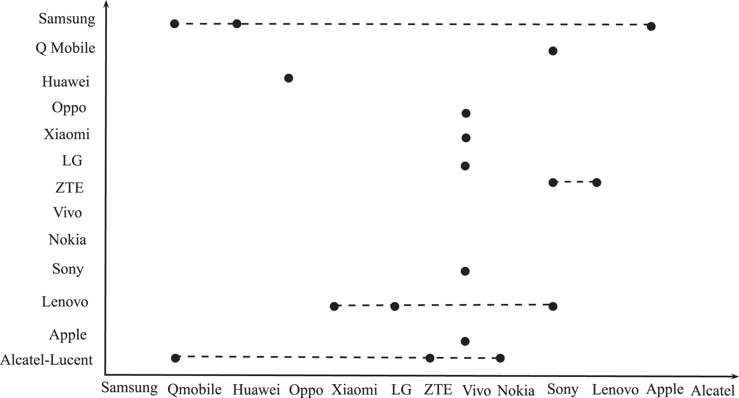
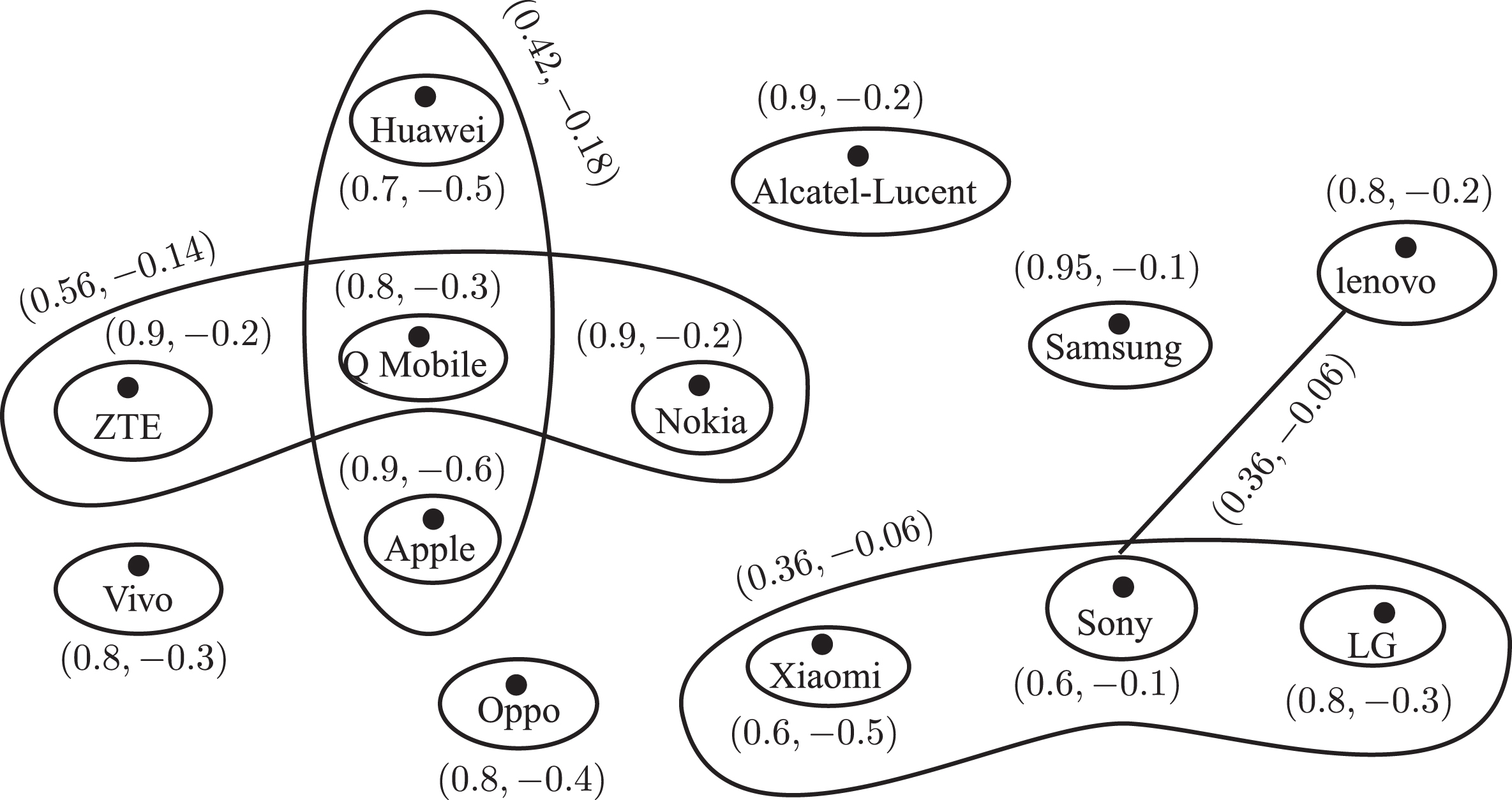
For example, the grade of membership of Samsung is (0.95, - 0.1) which indicates that 90% profit and 10% loss to Samsung company at every year. The directed arrow between Huawei and Samsung has a membership grade (0.6, - 0.1) which indicates that 60% import purchased and 10% import decline of Huawei by Samsung. The BF out neighborhood of each company is given in Table 9. Using Algorithm 3.1, the relationship between companies is given in Figure 5.2. By using relation 5.2, we compute the hyperedges of BF competition hypergraph also called BF rivalry hypergraph. Following are the hyperedges of BF competition hypergraph $CH (\vec{J})$ . f ^-1(Alcatel-Lucent) = {ZTE, Q Mobile, Nokia}, f ^-1(ZTE) = {Sony, Lenovo},

f ^-1(Lenovo) = {Xiaomi, Sony, LG}, f ^-1(Samsung) = {Huawei, Q Mobile, Apple}.

Table 9
BF out neighborhood of companies

Company N⁺ (y):y is company

Samsung ∅

Apple {Samsung, 0.8, -0.5}

Huawei {(Samsung, 0.6, -0.1)}

Oppo {(Huawei, 0.7, -0.3)}

Vivo {(Oppo, 0.8, -0.4),(Apple, 0.8, -0.3), (Sony, 0.6, -0.1), (LG, 0.7, -0.3), (Xiaomi, 0.6, -0.3)}

Xiaomi {(Lenovo, 0.6, -0.2)}

LG {(Lenovo, 0.7, -0.2)}

ZTE { (Alcatel-Lucent, 0.8, -0.1)}

Alcatel-Lucent ∅

Nokia {(Alcatel-Lucent,0.9, -0.2)}

Q Mobile { (Alcatel-Lucent, 0.7, -0.2), (Samsung, 0.7, -0.1)}

Sony {(Q Mobile, 0.7, -0.2), (ZTE, 0.6, -0.1), (Lenovo, 0.7, -0.5)}

Lenovo {(ZTE, 0.8, -0.1)}

Company	N⁺ (y):y is company
Samsung	∅
Apple	{Samsung, 0.8, -0.5}
Huawei	{(Samsung, 0.6, -0.1)}
Oppo	{(Huawei, 0.7, -0.3)}
Vivo	{(Oppo, 0.8, -0.4),(Apple, 0.8, -0.3), (Sony, 0.6, -0.1), (LG, 0.7, -0.3), (Xiaomi, 0.6, -0.3)}
Xiaomi	{(Lenovo, 0.6, -0.2)}
LG	{(Lenovo, 0.7, -0.2)}
ZTE	{ (Alcatel-Lucent, 0.8, -0.1)}
Alcatel-Lucent	∅
Nokia	{(Alcatel-Lucent,0.9, -0.2)}
Q Mobile	{ (Alcatel-Lucent, 0.7, -0.2), (Samsung, 0.7, -0.1)}
Sony	{(Q Mobile, 0.7, -0.2), (ZTE, 0.6, -0.1), (Lenovo, 0.7, -0.5)}
Lenovo	{(ZTE, 0.8, -0.1)}

The grade of membership of these hyperedges can be calculated by using Definition 3.1. The BF rivalry hypergraph is given in Figure 5.3. The grade of membership of each hyperedge among companies indicates the strength of competition among companies for purchase and decline of their products.

Now we discuss the strength of competition of each mobile company by using BF rivalry hypergraph. The strength of the competition of each mobile company is computed in Table 10 which indicates its competitive significance in the market. However, Table 10 indicates that Q Mobile is the most competitive mobile company in the business market.

Table 10

Strength of competition among companies

Company	Degree of Company	Strength of competition
ZTE	(0.56, - 0.14)	0.71
Nokia	(0.56, - 0.14)	0.71
Q Mobile	(0.98, - 0.32)	0.83
Apple	(0.42, - 0.18)	0.62
Huawei	(0.42, - 0.18)	0.62
Xiaomi	(0.36, - 0.06)	0.65
Sony	(0.72, - 0.12)	0.8
LG	(0.36, - 0.06)	0.65
Lenovo	(0.36, - 0.06)	0.65

Table 11

Strength of competition among companies

Company	Degree of Company	Strength of competition
ZTE	(1.28, - 0.3)	0.99
Nokia	(1.28, - 0.3)	0.99
Q Mobile	(2.1, - 0.67)	1.215
Apple	(0.98, - 0.51)	0.735
Huawei	(0.84, - 0.48)	0.68
Xiaomi	(0.72, - 0.24)	0.74
Sony	(1.14, - 0.19)	0.975
LG	(0.78, - 0.25)	0.765
Lenovo	(0.36, - 0.06)	0.65

Merits of the Proposed Model

The merits of the proposed model are as follows:

The proposed BF competition hypergraphs are a generalized case of BF competition graphs [5] and fuzzy competition hyperggraphs [24] to deal with bipolar competition in the form of BF hypergraphs instead of BF graphs. As, in BF graph, we usually miss some information that whether two or more objects satisfy a common competition and, in fuzzy competition hypergraphs, we miss the bipolar information of objects.

BF competition hypergraphs are used to compute the degree of competition, influence or power in any BF network and these degrees can be used to rank the objects in ascending or descending order.

The proposed BF competition hypergraphs can be extended to BF double competition hypergraphs to study the conflict and interest simultaneously in a single mathematical structure under BF environment.

6 Comparison analysis

In this section, we discuss the comparison of BF competition hypergraphs with BF competition graphs and fuzzy competition hypergraphs.

6.1 Comparison with bipolar fuzzy competition graphs

The idea of BF competition graphs successfully utilized in different real-world problems such as food webs, business trading, politics, wireless communication, and many others. But in all these applications, we consistently study pair-wise competition between objects. For instance, the BF competition graph of Figure 5.1 is given in Figure 6.1 which indicates the competition between two companies only. For a more detailed description of BF competition graphs we refer the readers to read [5 , 23].

Fig. 5.1

BF marketing digraph $\vec{J}$

Fig. 5.2

Representation of BF relation $\vec{N}$ of companies

Fig. 5.3

BF rivalry hypergraph

Fig. 6.1

BF rivalry graph

Fig. 6.2

BF food web digraphs

Using BF competition graph 6.1, we compute the strength of competition of each mobile company. In Table 11 numerical value of each company show its significant worth within business market. However, Table 11 indicates that Q Mobile is the most competitive mobile company in the business market.

Table 12 indicates the comparison between BF competition graph (existing model) and BF competition hypergraph (proposed model). It shows the same ranking of results through different techniques but the priorities of the proposed method are described as follows. In existing model, we discuss pairwise competition, relations, and influences among objects, and the ranking results of each object show its competitive worth just in pairwise rivalries. However, this model neglect some information whether there is a conflict or relation among more than two objects and also fails to tell the strength of competition of each object in group-wise rivalries. Thus, the existing model lacks a lot of important information and hides many errors and flaws. The proposed model permits handling this diversity and assist to approach such decision-making problems not only pair-wise but also in group-wise rivalries and relations. The other main reason to prefer the proposed model over existing model is that proposed model not only generalizes the existing model but also gives more accurate, precise, and error-free results regarding bipolarity. It shows the validity of the proposed method.

Table 12

Comparison of results of two different models

Company	BF competition graph [23]		Proposed model
	Degree of Company	Strength of competition	Degree of Company	Strength of competition
ZTE	(1.28, - 0.3)	0.99	(0.56, - 0.14)	0.71
Nokia	(1.28, - 0.3)	0.99	(0.56, - 0.14)	0.71
Q Mobile	(2.1, - 0.67)	1.215	(0.98, - 0.32)	0.83
Apple	(0.98, - 0.51)	0.735	(0.42, - 0.18)	0.62
Huawei	(0.84, - 0.48)	0.68	(0.42, - 0.18)	0.62
Xiaomi	(0.72, - 0.24)	0.74	(0.36, - 0.06)	0.65
Sony	(1.14, - 0.19)	0.975	(0.72, - 0.12)	0.8
LG	(0.78, - 0.25)	0.765	(0.36, - 0.06)	0.65
Lenovo	(0.36, - 0.06)	0.65	(0.36, - 0.06)	0.65

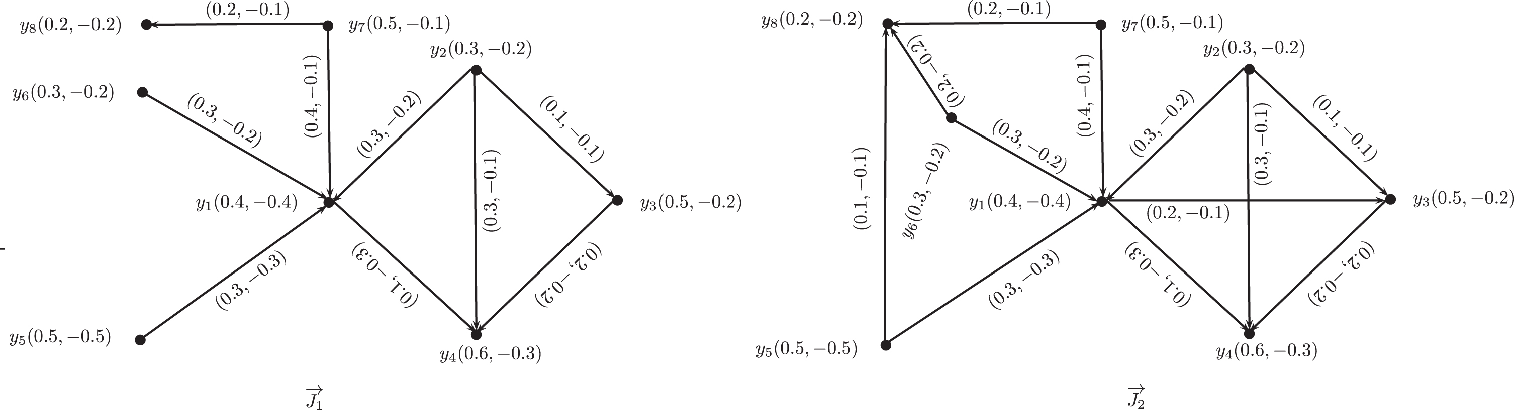
This example illustrates that BF competition hypergraphs yield a more detailed description than BF competition graphs in some cases. Consider the two different food webs $\vec{j_{1}}$ and $\vec{j_{2}} = \vec{j_{1}} + (\vec{1, 3}) + (\vec{5, 8}) + (\vec{6, 8})$ as shown in Figure 6.2. Suppose vertices of both BF digraphs represent the species and edge between two vertices $\vec{y_{2} y_{1}}$ represents y₂ preys y₁. The grade of membership of both BF digraphs indicate that species are healthy and unhealthy, respectively.

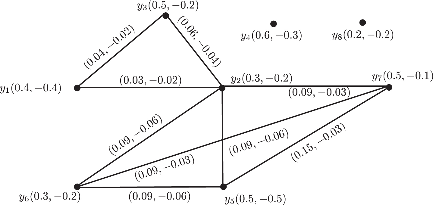
To compute the BF competition graphs of both $\vec{j_{1}}$ and $\vec{j_{2}}$ we refer the reader to [23]. The BF competition graphs of both $\vec{j_{1}}$ and $\vec{j_{2}}$ are same $C (\vec{j_{1}}) = C (\vec{j_{1}})$ as shown in Figure 6.3.

Fig. 6.3

BF competition graph

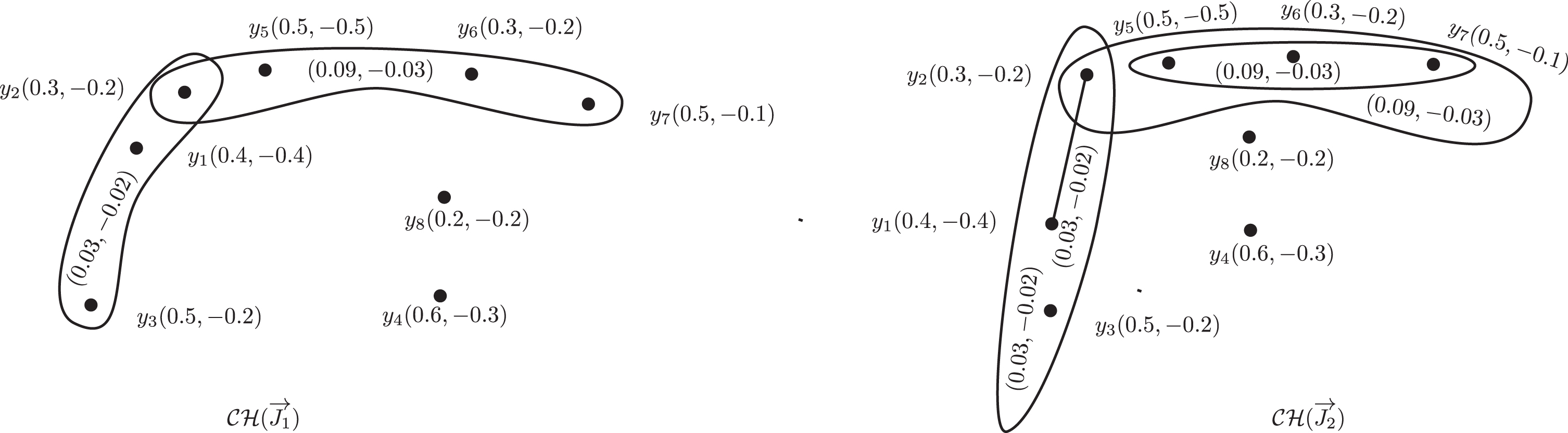
The edge between y₁ and y₂ shows that both species y₁ and y₂ have common prey y₄. After some variations in $\vec{J_{1}}$ (e.g y₅ preys y₈ in $\vec{J_{2}}$ but not in $\vec{J_{1}}$ and so on) there is no change in the BF competition graph corresponding to $\vec{J_{2}}$ . Consequently, the competition among species remains the same in both cases. On the other hand, BF competition hypergraphs corresponding to both $\vec{j_{1}}$ and $\vec{j_{2}}$ are different as shown in Figure 6.4. Both $CH (\vec{J_{1}})$ and $CH (\vec{J_{2}})$ yields different information. For instance, the hyperedge {y₂, y₅, y₆, y₇} of $CH (\vec{J_{1}})$ shows that there is a competition between four species y₂, y₅, y₆, and y₇ for common prey y₁. Furthermore, in $CH (\vec{J_{2}})$ the hyperedge {y₂, y₅, y₆, y₇} indicates that these species compete for y₁ and {y₅, y₆, y₇} compete for y₈. Consequently, in $CH (\vec{J_{1}})$ the species y₅, y₆, and y₇ compete only for one prey y₁ but in $CH (\vec{J_{2}})$ the species y₅, y₆, and y₇ compete for two different preys y₁ and y₈. Hence BF competition hypergraphs produced different results in different cases but BF competition graphs give the same result in different cases.

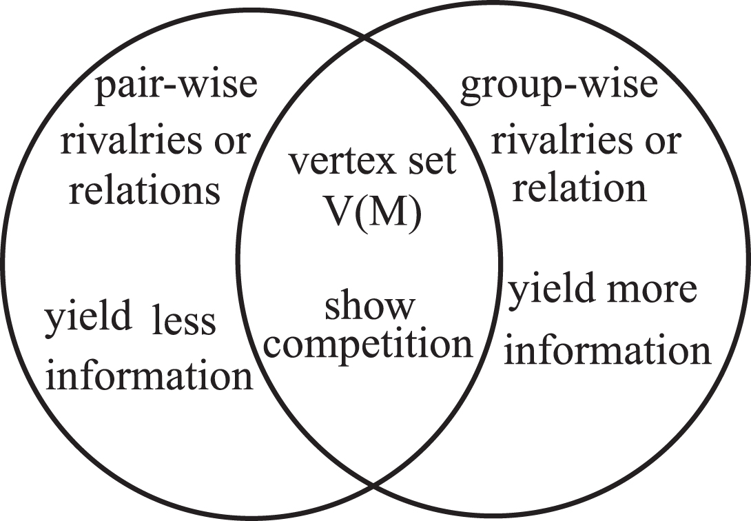
Following Figure 6.5 shows the similarities and differences between BF competition hypergraphs and BF competition graphs.

Fig. 6.4

BF competition hypergraphs

Fig. 6.5

$C (\vec{J})$ vs $CH (\vec{J})$

The vertex sets of both $C (\vec{J})$ and $CH (\vec{J})$ are same and both show the competition between objects. BF competition graphs manifest competition between only two objects, however, BF competition hypergraphs demonstrate the competition between three, four, and more objects. It is obvious that BF competition hypergraphs are generalized form of BF competition graphs. From above discussion, we can see that in some cases $C (\vec{J})$ gives the same information and results but $CH (\vec{J})$ provides different information and consequences in different cases. So in some cases, $C (\vec{J})$ yields less information in comparison with $CH (\vec{J})$ .

6.2 Comparison with fuzzy competition hypergraphs

Fuzzy competition hypergraph [24] is an efficient model for dealing with competitions and conflicts among objects based on uncertainty. Fuzzy competition hypergraphs have played an important role for solving decision-making problems including predator-prey relations in ecological niche, social networks, and business marketing. But in all these problems, the uncertainty was considered only in one direction. For instance, in competition among mobile companies, we can only represent the purchase or decline of their products by a common company through fuzzy numbers. These models lack some information regarding the double-sided thinking about the given situation. To deal with purchase as well as decline of their products by a common company, the proposed model provides a better illustration in form of positive and negative membership degrees.

7 Conclusions and future directions

The mathematical modeling based on bipolar fuzziness is an extremely useful tool and provides more flexible and accurate results as compared to the existing classical and fuzzy models. In this article, the concept of BF hypergraph is introduced to generalize the existing notions of fuzzy hypergraphs and BF competition graphs. The construction methods of BF competition hypergraphs and various new types of it by imposing appropriate conditions are defined and studied in detail. Certain novel concepts including BF open neighborhoods hypergraphs, BF closed neighborhoods hypergraphs, BF k -competition hypergraphs are discussed with certain interesting properties. The notion of BF competition hypergraph is illustrated with a real-world problem in business marketing and an algorithm is designed to show the strength of competition among vertices. This research work can be further extended to (i) Single-valued neutrosophic rough hyper graphs; (ii) q-rung orthopair fuzzy rough competition hypergraphs; (iii) Rough bipolar neutrosophic competition graphs.

Conflicts of Interest: The authors declare no conflict of interest.

Ethical approval: This article does not contain any studies with human participants or animals performed by any of the authors.

References

Akram

and Luqman

, Certain concepts of bipolar fuzzy directed hypergraphs, Mathematics 5(1) (2017), 1–18.

Akram

, Bipolar fuzzy graphs, Information Sciences 181(24) (2011), 5548–5564.

Akram

, Sarwar

and Dudek

W.A.

, Graphs for the analysis of bipolar fuzzy information, Studies in Fuzziness and Soft Computing, Springer, (2021). DOI:10.1007/978-981-15-8756-6.

Akram

and Luqman

, Fuzzy hypergraphs and related extensions, Studies in Fuzziness and Soft Computing, Springer, (2020). DOI: 10.1007/978-981-15-2403-5.

Al-shehri

N.O.

and Akram

, Bipolar fuzzy competition graphs, Ars Comb 121 (2015), 385–402.

Bhattacharya

, Some remarks on fuzzy graphs, Pattern Recognition Letters 6(5) (1987), 297–302.

Cohen

J.E.

, Interval graphs and food webs: a finding and a problem. Document 17696-PR, RAND Corporation, Santa Monica. (1968).

Dubois

and Prade

, Rough fuzzy sets and fuzzy rough sets, International Journal of General Systems 17(2-3) (1990), 191–209.

Garske

, Sonntag

and Teichert

H.M.

, Niche hypergraphs, Discussiones Mathematicae Graph Theory 36(4) (2016), 819–832.

10.

Kaufmann

, Introduction la thorie des sous-ensembles flous lusage des ingnieurs (Fuzzy sets theory). Paris: Masson. (1973).

11.

Lee-Kwang

and Lee

K.M.

, Fuzzy hypergraph and fuzzy partition. IEEE Transactions on Systems, Man and Cybernetics 25(1) (1995), 96–102.

12.

Lundgren

J.R.

, Food webs, competition graphs, competition-common enemy graphs, and niche graphs. In Applications of Combinatorics and Graph Theory to the Biological and Social Sciences, Springer, New York, NY, (1989), 221–243.

13.

Mordeson

J.N.

and Nair

P.S.

, Fuzzy graphs and fuzzy hypergraphs, Physica Verlag, Heidelberg, 1998; (2012). Second Edition 2001.

14.

Pawlak

, Rough sets, International Journal of Computer and Information Sciences 11(5) (1982), 341–356.

15.

Park

and Sano

, The double competition hypergraph of a digraph, Discrete Applied Mathematics 195 (2015), 110–113.

16.

Rashmanlou

, Samanta

, Pal

and Borzooei

R.A.

, A study on bipolar fuzzy graphs, Journal of Intelligent and Fuzzy Systems 28(2) (2015), 571–580.

17.

Rosenfeld

, Fuzzy Graphs; Fuzzy Sets and Their Applications, Academic Press: New York, NY, USA, (1975), 77–95.

18.

Samanta

and Pal

, Fuzzy k-competition graphs and p-competition fuzzy graphs, Fuzzy Information and Engineering 5(2) (2013), 191–204.

19.

Samanta

, Pal

and Pal

, Some more results on bipolar fuzzy sets and bipolar fuzzy intersection graphs, The Journal of Fuzzy Mathematics 22(2) (2014), 253–262.

20.

Samanta

, Akram

and Pal

, m-Step fuzzy competition graphs, Journal of Applied Mathe-matics and Computing 47(1-2) (2015), 461–472.

21.

Samanta

and Pal

, Bipolar fuzzy hypergraphs, International Journal of Fuzzy Logic Systems 2(1) (2012), 17–28.

22.

Sarwar

and Akram

, Certain algorithms for computing strength of competition in bipolar fuzzy graphs, International Journal of Uncertainty, Fuzziness and Knowledge-Based Systems 25(06) (2017), 877–896.

23.

Sarwar

and Akram

, Novel concepts of bipolar fuzzy competition graphs, Journal of Applied Mathematics and Computing 54(1) (2017), 511–547.

24.

Sarwar

, Akram

and Alshehri

N.O.

, A new method to decision-making with fuzzy competition hypergraphs, Symmetry 10(9) (2018), 404.

25.

Scott

D.D.

, The competition-common enemy graph of a digraph, Discrete Applied Mathematics 17(3) (1987), 269–280.

26.

Sonntag

and Teichert

H.M.

, Competition hypergraphs, Discrete Applied Mathematics 143(1-3) (2004), 324–329.

27.

Sonntag

and Teichert

H.M.

, Competition hypergraphs of digraphs with certain properties II. Hamiltonicity, Discussiones Mathematicae Graph Theory 28(1) (2008), 23–34.

28.

Wang

, Ma

, Xu

and Zhan

, Three-way multi-attribute decision making under hesitant fuzzy environments, Information Sciences 552 (2021), 328–351.

29.

, Zhan

, Ding

and Fujita

, A novel fuzzy rough set model with fuzzy neighborhood operators, Information Sciences 544 (2021), 266–297.

30.

Zadeh

L.A.

, Fuzzy sets, Information and Control 8(3) (1965), 338–353.

31.

Zadeh

L.A.

, Similarity relations and fuzzy orderings, Information Sciences 3(2) (1971), 177–200.

32.

Zhang

W.R.

, Bipolar fuzzy sets and relations: a computational framework for cognitive modeling and multiagent decision analysis. In NAFIPS/IFIS/NASA’94. Proceedings of the First International Joint Conference of The North American Fuzzy Information Processing Society Biannual Conference. The Industrial Fuzzy Control and Intellige (1994), (pp. 305–309). IEEE.

33.

Zhang

W.R.

, Bipolar fuzzy sets. In 1998 IEEE International Conference on Fuzzy Systems Proceedings, IEEE World Congress on Computational Intelligence (Cat. No. 98CH36228) (1998), (Vol. 1, pp. 835–840). IEEE.

34.

Zhang

, Zhan

and Wu

W.Z.

, On multi-criteria decision-making method based on a fuzzy rough set model with fuzzy alpha-neighborhoods, IEEE Transactions on Fuzzy Systems, (2020). DOI: 10.1109/TFUZZ.2020.3001670.

35.

Zhan

, Jiang

and Yao

, Three-way multi-attribute decision-making based on outranking relations, IEEE Transactions on Fuzzy Systems, (2020). DOI: 10.1109/TFUZZ.2020.3007423.

A framework of decision making based on bipolar fuzzy competition hypergraphs

Abstract

Keywords

1 Introduction

2 Preliminaries

Table 2 Adjacency matrix A y 1 y 2 ⋯ y n y 1 ( y 11 + , y 11 - ) ( y 12 + , y 12 - ) ⋯ ( y 1 n + , y 1 n - ) y 2 ( y 21 + , y 21 - ) ( y 22 + , y 22 - ) ⋯ ( y 2 n + , y 2 n - ) ⋮ ⋮ ⋮ ⋱ ⋮ y n ( y n 1 + , y n 1 - ) ( y n 2 + , y n 2 - ) ⋯ ( y nn + , y nn - )

6.1 Comparison with bipolar fuzzy competition graphs

7 Conclusions and future directions

References