Particle swarm optimization for the shortest path problem

Abstract

Solving the shortest path problem is very difficult in situations such as emergency rescue after a typhoon: road-damage caused by a typhoon causes the weight of the rescue path to be uncertain and impossible to represent using single, precise numbers. In such uncertain environments, neutrosophic numbers can express the edge distance more effectively: membership in a neutrosophic set has different degrees of truth, indeterminacy, and falsity. This paper proposes a shortest path solution method for interval-valued neutrosophic graphs using the particle swarm optimization algorithm. Furthermore, by comparing the proposed algorithm with the Dijkstra, Bellman, and ant colony algorithms, potential shortcomings and advantages of the proposed method are deeply explored, and its effectiveness is verified. Sensitivity analysis performed using a 2020 typhoon as a case study is presented, as well as an investigation on the efficiency of the algorithm under different parameter settings to determine the most reasonable settings. Particle swarm optimization is a promising method for dealing with neutrosophic graphs and thus with uncertain real-world situations.

Keywords

Interval-valued neutrosophic numbers neutrosophic graph particle swarm optimization algorithm shortest path problem

1 Introduction

The shortest path problem (SPP) is a fundamental combinatorial problem that appears in various scientific and engineering fields. The purpose of the SPP is to find the shortest path, i.e., the smallest weighted distance between the start and end points in a graph [1, 2]. In applications, the lengths and weights of the edges represent features such as time and cost. In the classic SPP, the distances between the nodes in the network are usually regarded as deterministic and represented by precise numbers. However, in most practical problems, the length and weight of an edge cannot be assigned exact values. An example is the network of routes used in rescue operations after a typhoon. Residents of coastal areas of China, one of the countries most affected by typhoons in the world, often face the threat of loss of life and property owing to severe storms and heavy rains and sometimes require rescue. Washed-out bridges and roads that are flooded and blocked by trees and debris mean that the rescue path after a disaster has many uncertain variables. The length of the rescue path cannot be given a definite value because of typhoon damage. This situation is a typical example of an SPP with inexact weight on the edges of the network graph, a problem that has attracted increasing attention from scholars all over the world.

Buckley and Jowers [3] introduced the concept of fuzzy logic into such SPPs. Subsequently, Deng et al. [4] proposed a fuzzy Dijkstra algorithm for SPPs in inaccurate environments and defined addition and sorting methods for fuzzy edge weights. Further, Biswas et al. [5] introduced an algorithm for finding the shortest path in intuitionistic fuzzy environments. Hu and Sotirov [6] derived several semidefinite programming relaxations for the quadratic SPP and proposed branch-and-bound algorithms to solve the SPP. Later, Zhang et al. [7] proposed a robust shortest path model that only requires partial distribution information about travel times, including the support set, mean, variance, and correlation matrix.

A neutrosophic set (NS) is an extension of an intuitionistic fuzzy set [8], which considers uncertainty and describes practical problems in more detail. In 1998, Smarandache [9] introduced neutrosophy. The NS concept involves three degrees of independence: true membership (T), uncertain membership (I), and false membership (F). Subsequently, the NS theoretical framework was gradually enriched. Ye [10] proposed the single-valued neutrosophic hesitant fuzzy set as a further generalization of the concepts of fuzzy, intuitionistic fuzzy, single-valued neutrosophic, hesitant fuzzy, and dual hesitant fuzzy sets. Wang et al. [11] described interval-valued NSs and logic in detail. Later, Peng [12] introduced the operations of multi-valued NSs and developed a comparison method based on related research of hesitant fuzzy sets and intuitionistic fuzzy sets. Meanwhile, Ye [13] proposed a trapezoidal NS, several operational rules, and score and accuracy functions for trapezoidal neutrosophic numbers (NNs). Nancy and Garg [14] proposed an improved score function for ranking NSs and applied it to decision-making process. More recently, Smarandache [15] proposed NeutroAlgebra, a generalization of partial algebra with uncertain opposites, and Mohanta et al [16]. presented an m-polar neutrosophic graph model. Son et al. [17] established some basic arithmetic operations of single-valued NNs. Meanwhile, Tey et al. [18] proposed a multi-criteria decision making method called the neutrosophic data analytical hierarchy process for the single-valued NS, and Dat et al. [19] introduced single-valued linguistic interval complex NS (ICNS) and interval linguistic ICNS and designed their operational rules. Further, Edalatpanah et al. [20] presented a new concept in NSs called the neutrosophic structured element.

Owing to the enrichment of NS theory, it is being increasingly used by many scholars to solve problems in their respective fields. For instance, Ridvan et al. [21] developed a method of solving multiple-attribute decision-making problems using single-valued or interval neutrosophic information, and Deli et al. [22] investigated multiple attribute decision-making problems in which both the attribute values and attribute weights of the alternatives are single-valued trapezoidal NNs. Broumi et al. [23] proposed an algorithm for finding the minimum spanning tree of an undirected neutrosophic weighted connected graph in which the edge weights are represented by interval-valued bipolar NNs. Meanwhile, Peng and Dai [24] presented an interval algorithm for decision making in a neutrosophic environment, and Deli et al. [25] proposed a ranking method for a single-valued NN and applied it to decision-making problems. Garg and Nancy [26] developed a nonlinear programming model based on the technique for order preference by similarity to ideal solution in an interval-valued neutrosophic environment. Faruk and Khizar [27] introduced some novel operations on neutrosophic matrices, and Bolturk and Kahraman [28] proposed a new interval-valued neutrosophic analytic hierarchy process with a cosine similarity measure. Meanwhile, Pramanik et al. [29] extended the VIseKriterijumska Optimizacija I Kompromisno Resenje strategy for multi-attribute decision-making problems to a trapezoidal NN environment. Deli [30] proposed a new method of expanding and reducing classical neutrosophic soft sets based on linguistic modifiers and gave an example of the application of the method. Deli [31] also proposed single-valued trapezoidal neutrosophic operators and applied them to decision-making problems, and Deli and Suba [32] together applied a weighted geometric operator with single-valued NNs to decision-making problems. Basset et al. [33] proposed a decision-making technology to enable decision makers to select the most appropriate projects and to check for consistency and calculate the degree of consensus among expert opinions in a neutrosophic environment. Recently, Fu and Ye [34] developed a PC risk assessment approach in an interval-valued neutrosophic environment. Schweizer [35] proposed the uncertain factors that can be considered in the process of establishing models and presented a formula to transform models into neutrosophic representations. Edalatpanah [36] developed a direct algorithm for solving neutrosophic linear-programming problems, in which the variables and right side are represented by a triangular NNs. Further, Dey et al. [37] proposed a new genetic algorithm to solve the fuzzy minimum spanning tree problem. Son et al. [38] studied the optimal control problem using fractional and partial differential equations in a minimum quadratic objective function in the framework of a neutrosophic environment and granular computing. Thong et al. [39] developed some operators and a technique for order of preference by similarity to ideal solution method to address simultaneous changes in criteria, alternatives, and decision-makers by time based on an extension of dynamic internal-valued NSs. Further, Can et al. [40] proposed a new method of classifying harmful domain names using NSs and highlighted the importance of neutrosophication of statistical data in study to assess the symptoms related to reproductive tract infections or sexually transmitted infections among women by sampling estimation [41]. In medicine, Basset et al. [42] proposed a novel framework based on computer supported diagnosis and the Internet of Things to detect and monitor heart failure patients. Jha et al. [43] put forth a novel image segmentation concept using NSs. Long et al. [44] presented a fuzzy clustering algorithm utilizing a neutrosophic association matrix. Meanwhile, Edalatpanah et al. [45] proposed an input-oriented data envelopment analysis model with simplified NNs and present a new strategy to solve it. More recently, Yang et al. [46] introduced a model of data envelopment analysis in the context of NSs and sketched an innovative process to solve it.

In practical applications, the edge weights in the SPP also encounter uncertain situations. NS theory is increasingly used by many scholars to solve the SPP. For instance, Broumi et al. [47] solved the SPP on a single-valued neutrosophic graph. Yang et al. [48] proposed a fuzzy reliable SPP under a mixed fuzzy environment; however, Kumar et al. [49] noted that Yang et al. had used some mathematically incorrect assumptions in the mixed fuzzy domain, which are not true in fuzzy environments. Kumar et al. [50] also presented an SPP model with various arrangements of integer-valued trapezoidal and triangular NNs. Smarandache [51] used trapezoidal fuzzy NNs to determine the shortest path, and Kumar et al. [52] proposed an algorithm for solving the SPP in a trapezoidal fuzzy neutrosophic environment. Broumi et al. [53] presented an extended version of the Dijkstra algorithm to find the shortest path in a network in which the edge weights are characterized by interval-valued NNs. Later, Tan et al. [54] proposed an extended dynamic programming method for solving the SPP to obtain the shortest path and shortest path length, and Broumi et al. [55] proposed a score function for interval-valued NNs and used it to solve the SPP. Moreover, they considered the SPP with the Bellman algorithm for a network using interval-valued NNs. The dynamic programming algorithm is similar to the Bellman algorithm, starting from the ending and starting point of the path, but the time cost is higher than Dijkstra algorithm. Chakraborty [56] applied the development score and accuracy functions of a pentagonal neural network to the SPP. Recently, Yang et al. [57, 58] proposed the use of circle-breaking and the ant colony algorithm to solve the SPP of interval neutrosophic graphs and employed various scoring functions to verify the stability of the algorithm. The ant colony algorithm is robust; however, the iteration process is relatively long: for a complex neutrosophic graph, hundreds of iterations are usually required to obtain the optimal solution.

In this paper, particle swarm optimization (PSO) was used to solve the SPP of an interval-valued neutrosophic graph. PSO [59] is a random search algorithm based on group cooperation developed by simulating the foraging behavior of birds. It is a kind of uncertain algorithm that embodies the biological mechanisms of natural creatures [60]. Compared with traditional algorithms, it is more suitable for solving the SPP in the case of no human intervention after a typhoon disaster. In addition, PSO uses a mechanism through which all particles share information [61 –63]. Compared with the mechanism of ants that do not share information with one another in the ant colony algorithm [58], PSO has a higher convergence efficiency.

The remainder of this paper is organized as follows. Section 2 briefly introduces some basic definitions and operation rules of NS, single-valued NNs, and interval-valued NNs. Section 3 describes the SPP in the context of emergency rescue. Section 4 presents the quantification process of an interval-valued neutrosophic graph, and Section 5 provides the detailed calculation steps of PSO. Section 6 discusses a typhoon disaster rescue example to illustrate the applicability of the proposed method and provides a comparative analysis to verity the advantages of the proposed method. Finally, Section 7 summarizes the conclusions.

2 Theoretical basis

This section briefly introduces some basic concepts of NSs, as well as the four arithmetic operations, scoring functions, and ranking methods of interval-valued NNs.

2.1 NS

Definition 1. ([9]) Let X be an object set, and x be any element in X; an NS A on X can be represented by the truth membership T_A (x), indeterminacy membership I_A (x), and falsity membership F_A (x), where T_A (x), I_A (x), and F_A (x) are standard or non-standard real subsets of [0, 1], and 0^- ≤ sup T_A (x) + sup I_A (x) + sup F_A (x) ≤3⁺.

2.2 Interval-valued NNs

Definition 2. ([10]) Let X be a domain; then, a single-valued NN $\tilde{N}$ in X can be expressed as

$\tilde{N} = {〈 x, T_{\tilde{N}} (x), I_{\tilde{N}} (x), F_{\tilde{N}} (x) 〉 | x \in X},$ (1) where $T_{\tilde{N}} (x) \in [0, 1]$ , $I_{\tilde{N}} (x) \in [0, 1],$ and $F_{\tilde{N}} (x) \in [0, 1]$ .

Definition 3. ([11]) If X is a domain, then an interval-valued NN $\tilde{N}$ in X can be expressed as

$\tilde{N} = {〈 x, T_{\tilde{N}} (x), I_{\tilde{N}} (x), F_{\tilde{N}} (x) 〉 | x \in X},$ (2) where $T_{\tilde{N}} (x) \subseteq [0, 1]$ , $I_{\tilde{N}} (x) \subseteq [0, 1]$ , and $F_{\tilde{N}} (x) \subseteq [0, 1]$ are interval numbers. Now let $T_{\tilde{N}} (x) = [T_{\tilde{N}}^{L} (x)$ , $T_{\tilde{N}}^{U} (x)]$ , where $0 \leq T_{\tilde{N}}^{L} (x) ≺ T_{\tilde{N}}^{U} (x) \leq 1$ . Similarly, $I_{\tilde{N}} (x) = [I_{\tilde{N}}^{L} (x), I_{\tilde{N}}^{U} (x)]$ , where $0 \leq I_{\tilde{N}}^{L} (x) ≺ I_{\tilde{N}}^{U} (x) \leq 1$ , and $F_{\tilde{N}} (x) = [F_{\tilde{N}}^{L} (x), F_{\tilde{N}}^{U} (x)]$ , where $0 \leq F_{\tilde{N}}^{L} (x) ≺ F_{\tilde{N}}^{U} (x) \leq 1$ .

Definition 4. ([11]) If ${\tilde{N}}_{1} = 〈 [a_{1}, a_{2}], [b_{1}, b_{2}], [c_{1}, c_{2}] 〉$ and ${\tilde{N}}_{2} = 〈 [d_{1}, d_{2}], [e_{1}, e_{2}], [f_{1}, f_{2}] 〉$ are two interval-valued NNs; then, ${\tilde{N}}_{1} \oplus {\tilde{N}}_{2} = 〈 \begin{matrix} [\begin{matrix} a_{1} + d_{1} - a_{1} d_{1}, \\ a_{2} + d_{2} - a_{2} d_{2} \end{matrix}], \\ [b_{1} e_{1}, b_{2} e_{2}], \\ [c_{1} f_{1}, c_{2} f_{2}] \end{matrix} 〉$ (3) ${\tilde{N}}_{1} \otimes {\tilde{N}}_{2} = 〈 \begin{matrix} [a_{1} d_{1}, a_{2} d_{2}], \\ [\begin{matrix} b_{1} + e_{1} - b_{1} e_{1}, \\ b_{2} + e_{2} - b_{2} e_{2} \end{matrix}], \\ [\begin{matrix} c_{1} + f_{1} - c_{1} f_{1}, \\ c_{2} + f_{2} - c_{2} f_{2} \end{matrix}] \end{matrix} 〉$ (4) $λ {\tilde{N}}_{1} = 〈 \begin{matrix} [\begin{matrix} 1 - (1 - a_{1})^{λ}, \\ 1 - (1 - a_{2})^{λ} \end{matrix}], \\ [b_{1}^{λ}, b_{2}^{λ}], \\ [c_{1}^{λ}, c_{2}^{λ}] \end{matrix} 〉$ (5) ${\tilde{N}}_{1}^{λ} = 〈 \begin{matrix} [a_{1}^{λ}, a_{2}^{λ}], \\ [\begin{matrix} 1 - (1 - b_{1})^{λ}, \\ 1 - (1 - b_{2})^{λ} \end{matrix}], \\ [\begin{matrix} 1 - (1 - c_{1})^{λ}, \\ 1 - (1 - c_{2})^{λ} \end{matrix}] \end{matrix} 〉 .$ (6)

2.3 Ranking function

Definition 5. ([15]) $\tilde{N} = 〈 [a_{1}, a_{2}], [b_{1}, b_{2}], [c_{1}, c_{2}] 〉$ is an interval-valued NNs, and its score function can be expressed as

$S (\tilde{N}) = (\frac{1}{4}) \times (\begin{matrix} 2 + a_{1} + a_{2} - 2 b_{1} \\ - 2 b_{2} - c_{1} - c_{2} \end{matrix}) .$ (7)

Definition 6. ([55]) ${\tilde{N}}_{1} = 〈 [a_{1}, a_{2}], [b_{1}, b_{2}], [c_{1}, c_{2}] 〉$ and ${\tilde{N}}_{2} = 〈 [d_{1}, d_{2}], [e_{1}, e_{2}], [f_{1}, f_{2}] 〉$ are two interval-valued NNs, and $S ({\tilde{N}}_{1})$ and $S ({\tilde{N}}_{2})$ are the score functions of ${\tilde{N}}_{1}$ and ${\tilde{N}}_{2}$ , respectively. The ordering relationships of the interval-valued NNs is as follows:

if $S ({\tilde{N}}_{1}) ≻ S ({\tilde{N}}_{2})$ , then ${\tilde{N}}_{1} ≻ {\tilde{N}}_{2}$ ;

if $S ({\tilde{N}}_{1}) ≺ S ({\tilde{N}}_{2})$ , then ${\tilde{N}}_{1} ≺ {\tilde{N}}_{2}$ ;

if $S ({\tilde{N}}_{1}) = S ({\tilde{N}}_{2})$ , then ${\tilde{N}}_{1} = {\tilde{N}}_{2}$ .

3 SPP in emergency decision making

Typhoons are characterized by unpredictable location and extent of damage, unpredictable scope and development, and uncertainties in the extent of damage to transportation facilities and roads. Emergency rescue after disasters requires decision makers to respond rapidly so that the rescue team and rescue materials reach the disaster site as soon as possible. An incorrect decision causing a delay can make the rescue attempt useless.

Generally, there are two objective functions in an emergency-system material-scheduling model: the rescue time and cost minimization functions. The former is often directly related to the success or failure of the rescue and was therefore chosen as the main objective function in the present work. When the rescue team has a fixed preparation time, the shortest rescue time is simply the shortest transportation time, and finding it is equivalent to finding the shortest path.

Typhoon disaster rescue thus differs from general enterprise logistics. The disaster relief team faces many uncertain factors during the journey, such as road-water accumulation after the disaster, bridge damage, and possibly landslides on mountainside roads. The size determines the level interval and uses the sophistication number in the interval to describe the path weight.

The traditional SPP is a combinatorial optimization problem that may be either single-source (involving finding the shortest path from a given point to the rest of the graph) or multiple-source (involving finding the shortest path between every pair of vertices in the graph). The current solutions to such problems are based on the classic Dijkstra and Bellman algorithms. In practical applications, an urban road network is generally represented by a geographical map. To find the best path, however, this map must be abstracted into a formal graph, with travel conditions and other factors encoded as edge weights on the arcs connecting the vertices. The SPP algorithm discussed here is primarily intended for application to directed graphs for which the weights of all arcs are interval-valued NNs.

4 Interval-valued neutrosophic graph in SPP

The starting point of the rescue team, destinations where victims await rescue, and various traffic points along the route can be represented abstractly as graph vertices. A disaster area composed of n locations and its network topology can be abstracted as a directed graph G (V, E), where the point set V = {v₁, v₂, ⋯⋯ v_n} represents the n points of significance for the mission, and the edge set E ⊆ V × V represents the directed connections between these vertices. A directed edge (i, j) ∈ E represents the path from point i to point j; node i is called the parent node, and node j is called a child node. A multi-step directed path from i to j can be represented as a set of directed edges in the form (i, i₂) , (i₂, i₃) , ⋯⋯ , (i_k, j) in a directed graph. The number of paths from one node to another varies according to the strength of the connectivity of the directed graph.

To make the best decision, it is necessary to consider the length and condition of the path, the transportation capacity, and factors such as the geographic location, terrain, and degree of damage caused by the disaster. Considering the amount of uncertain information, by requantizing the edge weights into an interval NNs, the rescue graph can be requantized into an interval neutrosophic graph.

5 Shortest path on interval neutrosophic graph via PSO

PSO randomly obtains the number of particles (and paths) particle_num, and each particle compares all the positions it flies over, finds the path with the smallest path score function, and obtains particle_num local optimal solutions pBest_i, among which the smallest local optimal solution is defined as the global optimal solution gBest. The flight speed of each particle is updated so that all particles slowly tend to gBest. In the iterative process, pBest_i and gBest are optimized by continuously modifying the particle flight speed, and finally all pBest_i converge to gBest. After each iteration, the particle velocity is adjusted according to the current extreme values using

$\begin{matrix} v_{i + 1} & = w \times v_{i} \\ + c_{1} \times random () \times (pBest - x_{i}) \\ + c_{2} \times random () \times (gBest - x_{i}) \end{matrix}$ (8) and

$x_{(i + 1)} = x_{i} + v_{(i + 1)},$ (9) where w is the inertia weighting coefficient of the particle flight, v_i is the flying speed of the particle after iterating i times, x_i is the position of the particle after iterating i times, c₁ is the particle self-acceleration weighting coefficient, c₂ is the global acceleration weighting coefficient, pBest is the current local optimal solution passed, gBest is the optimal solution for all particles, and random() is a random constant with a value in the range (0, 1). The two random constants in the formula are independent of each other. The flight speeds and positions of the particles are constantly updated so that the particles gradually tend to the global optimal solution. The specific steps are as follows:

Step 1: Initialize the feasible solution set Φ from the starting point to the ending point according to the side length of the neutrosophic diagram, particle_num, c₁, c₂, and w.

Step 2: Initialize the random position $X_{j}^{0}$ and velocity $V_{j}^{0}$ of each particle, the optimal solution pBest_j =fitness ( $X_{j}^{0}$ ) passed by the particle j, and the optimal solution _gBest⁰ = Min ( _p ${Best}_{j}^{0}$ ), j ∈ [0, particle_num) passed by all particles.

Step 3: Calculate the fitness value $fitness (X_{j}^{k}), k \in (0, N)$ of each particle after the first iteration.

Step 4: Compare the fitness value of each particle with that at its historical best position. If the former is better than the latter rtreat the current position as the best.

Step 5: Compare the local optimal solution for each particle with the best position gBest experienced by the world. If the latter is better than the former rreset pBest to gBest.

Step 6: Use Eqs. (8) and (9) to calculate $V_{j}^{(k + 1)}$ and $X_{j}^{(k + 1)}$ .

Step 7: If the local optimal solution of each particle converges to the global optimal solution rno new local optimal solution will appear rand the global optimal solution will also stabilize at a certain value gBest. Then rthe algorithm ends. Otherwise rset k = k + 1 and go to Step 3.

Figure 1 shows the flowchart of the algorithm.

Fig. 1

Flow chart of PSO.

6 Case study and comparative analysis

This section presents a specific case and its sensitivity analysis ras well as a comparison and analysis of the proposed PSO method with the current mainstream algorithms.

6.1 Case analysis

China is one of the countries most severely affected by typhoons. Fujian Province is located in the southeast coastal area of China ron the path of many typhoons and close to their source. When a typhoon makes landfall rthe severe storms and heavy rain not only pose huge threats to human life and property rbut also cause major problems for post-disaster rescue work by severely damaging roads and bridges. For instance rTyphoon Hagupit made landfall on the coast of Yueqing City rZhejiang Province rat around 3:30 a.m. on August 4 r2020. The maximum wind force near the center was level 13 (38 m/s). The storm then passed through Zhejiang and the two provinces of Jiangsu and Jiangsu. By 6:00 a.m. on August 5 r2020 rthe typhoon had moved from Yancheng rJiangsu rto the surface of the Yellow Sea rwhere it strengthened again. Zhejiang rFujian rShanghai rand other provinces and cities were all affected. Bridge damage and road blockage by floodwater rmud rfallen trees rand rockslides increased the difficulty of post-disaster rescue work rin that it was impossible to assign precise weights to rescue-path segments for the post-disaster response to Typhoon Hagupit.

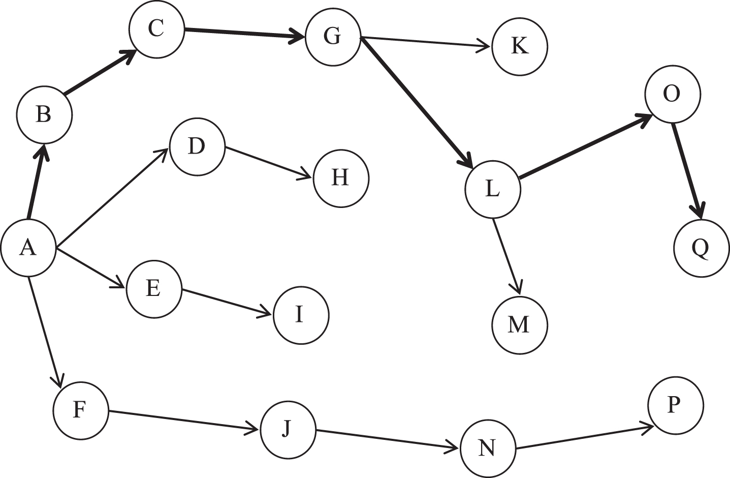
Figure 2 depicts the topological structure of the road network during this period, and Table 1 lists the side lengths. A rescue team in Fuzhou must start from point A and reach point Q to rescue trapped residents. Therefore, they must determine the shortest path from starting point A to ending point Q. The sequence can be summarized as follows:

Fig. 2

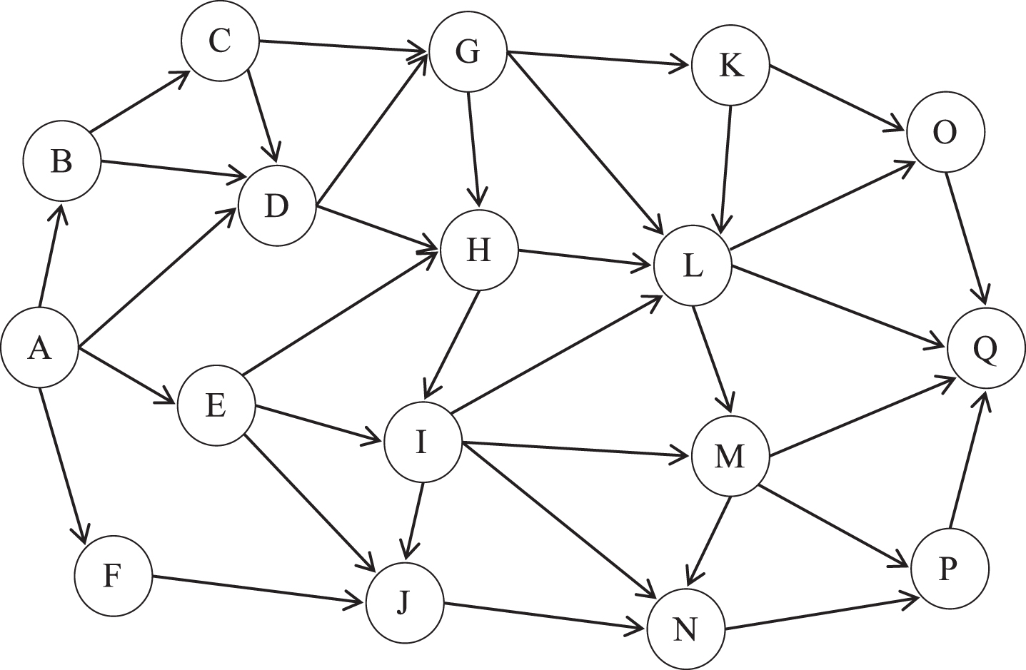
Interval-valued neutrosophic graph.

Table 1

Edge weights as interval-valued NNs

Edges	Interval-valued neutrosophic distance	Edges	Interval-valued neutrosophic distance
AB	< [0.1, 0.4], [0.5, 0.7], [0.4, 0.7]>	HL	< [0.3, 0.6], [0.2, 0.7], [0.2, 0.5]>
AD	< [0.5, 0.9], [0.3, 0.6], [0.1, 0.3]>	IJ	< [0.1, 0.4], [0.2, 0.7], [0.4, 0.8]>
AE	< [0.4, 0.8], [0.1, 0.5], [0.1, 0.4]>	IL	< [0.4, 0.7], [0.2, 0.6], [0.1, 0.3]>
AF	< [0.1, 0.3], [0.2, 0.4], [0.4, 0.6]>	IM	< [0.3, 0.7], [0.1, 0.5], [0.3, 0.5]>
BC	< [0.1, 0.4], [0.2, 0.5], [0.4, 0.7]>	IN	< [0.2, 0.4], [0.2, 0.5], [0.5, 0.9]>
BD	< [0.2, 0.6], [0.2, 0.6], [0.5, 0.8]>	JN	< [0.1, 0.5], [0.2, 0.6], [0.4, 0.8]>
CD	< [0.3, 0.5], [0.2, 0.6], [0.3, 0.5]>	KL	< [0.4, 0.9], [0.2, 0.6], [0.1, 0.5]>
CG	< [0.1, 0.3], [0.1, 0.6], [0.4, 0.7]>	KO	< [0.6, 0.8], [0.1, 0.5], [0.2, 0.3]>
DG	< [0.2, 0.4], [0.2, 0.6], [0.3, 0.7]>	LM	< [0.1, 0.3], [0.4, 0.7], [0.4, 0.6]>
DH	< [0.3, 0.5], [0.3, 0.7], [0.1, 0.3]>	LO	< [0.2, 0.5], [0.4, 0.6], [0.3, 0.6]>
EH	< [0.5, 0.7], [0.3, 0.6], [0.1, 0.3]>	LQ	< [0.6, 0.9], [0.3, 0.5], [0.1, 0.2]>
EI	< [0.4, 0.6], [0.2, 0.6], [0.2, 0.5]>	MN	< [0.1, 0.3], [0.1, 0.4], [0.3, 0.6]>
EJ	< [0.1, 0.3], [0.3, 0.5], [0.5, 0.7]>	MP	< [0.2, 0.6], [0.2, 0.5], [0.4, 0.5]>
FJ	< [0.2, 0.3], [0.2, 0.6], [0.4, 0.5]>	MQ	< [0.5, 0.8], [0.3, 0.7], [0.2, 0.4]>
GH	< [0.3, 0.8], [0.1, 0.4], [0.1, 0.6]>	NP	< [0.2, 0.5], [0.1, 0.3], [0.4, 0.7]>
GK	< [0.6, 0.9], [0.2, 0.6], [0.1, 0.2]>	OQ	< [0.1, 0.4], [0.2, 0.6], [0.4, 0.7]>
GL	< [0.2, 0.5], [0.3, 0.6], [0.1, 0.6]>	PQ	< [0.2, 0.5], [0.2, 0.5], [0.4, 0.6]>
HI	< [0.4, 0.9], [0.1, 0.5], [0.1, 0.6]>

Step 1: Initialize the parameters in the PSO: Set particle _ num = 5, c₁ = 2, c₂ = 2, and w = 1.4.

Step 2: Initialize the position $X_{j}^{0}$ and velocity $V_{j}^{0}$ of each particle. The first position and speed were generated randomly as $X_{j}^{0} = {58, 18, 50, 18, 24}, j \in {1, 2,$ $3, 4, 5}, V_{j}^{0} = {3, 1, 16, 20, 14}, j \in {1, 2, 3, 4,$ 5}, respectively.

The initial value of the optimal solution passed by each particle is p ${Best}_{j}^{0}$ =fitness ( $X_{j}^{0}$ ) = {0.96429, 0.95425, 0.95383, 0.95425, 0.92034}, and the initial value of the global optimal solution is gBest⁰= Min (p ${Best}_{j}^{0}$ )=0.92034.

Step 3: Calculate the next-step velocity of the particle from its initial position and velocity, $V_{j}^{1} = {19, 67,$ 27, - 12, - 9} , j ∈ {1, 2, 3, 4, 5} according to Eq. (8) and calculate the next position $X_{j}^{1} = X_{j}^{0} + V_{j}^{1} = {77, 85, 77, 6, 15}, j \in {1, 2, 3, 4, 5}$ of each particle according to Eq. (9). The fitness value of each particle after the first iteration is $fitness (X_{j}^{1}) = {0.95108, 0.90718, 0.95108, 0.90151, 0.89589}, j \in {1, 2,$ 3, 4, 5}.

Step 4: Compare the fitness value $fitness (X_{j}^{1})$ of the particle after the first iteration with the initial local optimal solution _p ${Best}_{j}^{0}$ , and update the local optimal solution p ${Best}_{j}^{1}$ = Min ( _p ${Best}_{j}^{0}$ , fitness ( $X_{j}^{1}$ )) ={ 0.95108, 0.90718, 0.95108, 0.90151, 0.89589 }.

Step 5: Update the global optimal solution _gBest¹= Min ( _p ${Best}_{j}^{1}$ )=0.89589.

Step 6: Update the particle velocity $V_{j}^{2} = {- 15, 5,$ -15, 10, 1} , j ∈ {1, 2, 3, 4, 5} according to Eq. (8) and update the particle position $X_{j}^{2} = X_{j}^{1} + V_{j}^{2} = {62, 80, 62, 16, 16}, j \in {1, 2, 3, 4, 5}$ according to Eq. (9).

Step 7: Determine whether the algorithm satisfies the termination condition. Because all items in _p ${Best}_{j}^{1}$ are not all equal to gBest¹, it is necessary to go to Step 3 to enter the next iteration. At the 68th iteration, p ${Best}_{j}^{68}$ = Min (p ${Best}_{j}^{67}$ , fitness ( $X_{j}^{68}$ )) = {0.84097, 0.84097, 0.84097, 0.84097, 0.84097 }, the local optimal solution of each particle is equal to gBest⁶⁸, which is therefore the weight of the shortest path. The corresponding shortest path is A->B->C->G->L->O->Q, as shown in bold in Fig. 3. The edge weight is $〈 \begin{matrix} [0.5801, 0.9622], \\ [0.00024, 0.04536], \\ [0.00077, 0.08644] \end{matrix} 〉$ , and the score function value is 0.84097. Table 2 presents the convergence of the score functions of the local optimal solutions.

Fig. 3

Shortest path through the graph in Fig. 2.

Table 2

Local optimal solutions for each particle

Iteration times	pBest₁	pBest₂	pBest₃	pBest₄	pBest₅	gBest
1	0.95108	0.90718	0.95108	0.90151	0.89589	0.89589
2	0.95108	0.90718	0.95108	0.90151	0.89589	0.89589
3	0.95108	0.90718	0.95108	0.90151	0.89589	0.89589
4	0.85933	0.88667	0.95108	0.90151	0.89589	0.85933
5	0.85933	0.88667	0.92688	0.89589	0.89589	0.85933
6	0.85933	0.88667	0.84097	0.89589	0.89589	0.84097
7	0.85933	0.88667	0.84097	0.89589	0.89589	0.84097
8	0.85933	0.88667	0.84097	0.89589	0.89400	0.84097
9	0.85933	0.88667	0.84097	0.89589	0.89400	0.84097
10	0.85933	0.85933	0.84097	0.89589	0.89400	0.84097
⋯	⋯	⋯	⋯	⋯	⋯	⋯
64	0.84237	0.84097	0.84097	0.84097	0.84097	0.84097
65	0.84237	0.84097	0.84097	0.84097	0.84097	0.84097
66	0.84237	0.84097	0.84097	0.84097	0.84097	0.84097
67	0.84237	0.84097	0.84097	0.84097	0.84097	0.84097
68	0.84097	0.84097	0.84097	0.84097	0.84097	0.84097

Figure 4 graphically depicts the convergence of the scores in Table 2.

Fig. 4

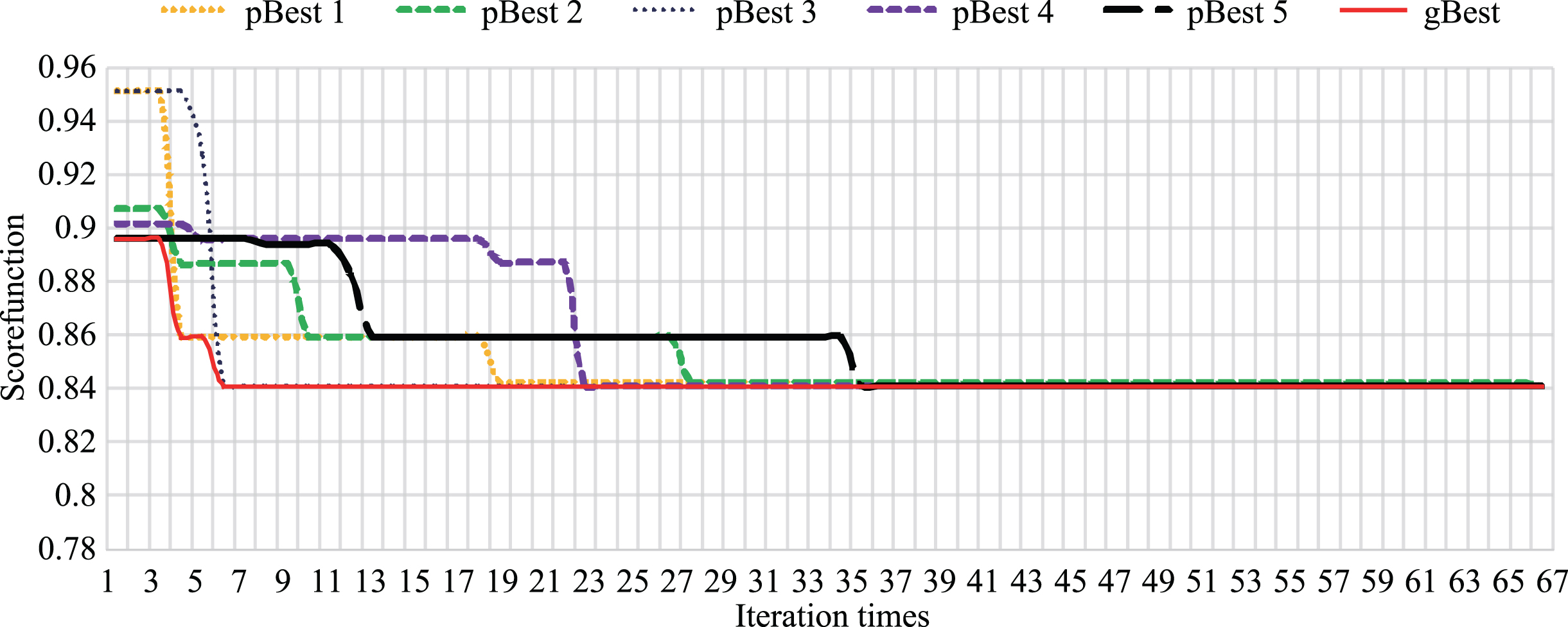
Convergence of local optimal solutions for five particles.

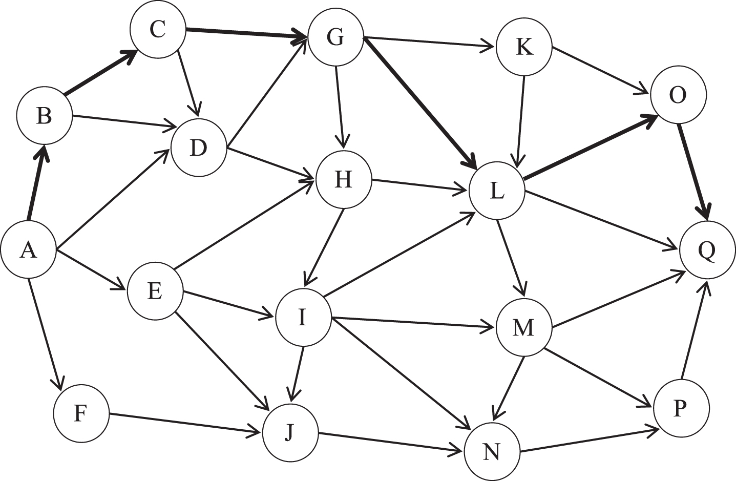
From Fig. 4, we can see that all five particles converge to the same optimal solution. When the number of iterations reaches 68, all particles converge to a path with a score function of 0.84097, which is the shortest path A->B->C->G->L->O->Q required by the system.

6.2 Sensitivity analysis

To find a reasonable setting of the parameters in the PSO, we studied the influence of each parameter on the efficiency of the algorithm. The specific method was to keep all the parameters but one unchanged, make the change in the single variable parameter take a value in a certain interval, and repeat the experiment 250 times for different values each time. The effect of this parameter on the efficiency of the algorithm was analyzed using the experimental data from the case discussed in Section 6.1. The experimental hardware is listed in Table 3.

Table 3
Main hardware parameters of the experiment

Hardware Hardware parameters

CPU Intel i7-10700F, 8 cores 16 threads

RAM Kingston DDR4 2400 Hz 32 GB

Graphics card NVIDIA GTX 1660 super 6 GB

Hard disk Kingston SSD 2 TB

Hardware	Hardware parameters
CPU	Intel i7-10700F, 8 cores 16 threads
RAM	Kingston DDR4 2400 Hz 32 GB
Graphics card	NVIDIA GTX 1660 super 6 GB
Hard disk	Kingston SSD 2 TB

6.2.1 Number of particles

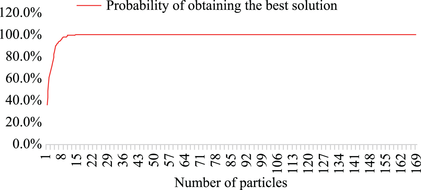
Assume c₁ = 2, c₂ = 2, w = 1.4. The number of particles particle_num is a value in the interval [1, 175]. Depending on the number of particles, the number of iterations required for the algorithm to obtain the optimal solution varies. For each of the 250 repetitions of the experiment, we recorded the number of iterations required for convergence for one to 175 particles (Table 3). When the number of iterations exceeded 3000 and the optimal solution could not be obtained, the program was forced to exit the iteration, and the number of iterations was recorded as “max, ” which means that the experiment only found the local optimal solutions.

According to the data in Table 4, as the number of particles increases, the number of occurrences of “max” decreases, which means that the program becomes increasingly successful at finding the optimal solution.

Table 4
Number of iterations for convergence in 250 experiments as function of number of particles

Number of particles 1 2 3 4 5 6 7 8 ⋯ 243 244 245 246 247 248 249 250

1 46 87 max max 1716 max 117 2481 ⋯ 1 max max max 5 max max 44

2 2157 2827 7 12 41 28 max max ⋯ 9 max 9 19 18 475 39 max

3 9 255 22 36 87 2 max 17 ⋯ max 20 max 15 max 2884 58 max

4 24 27 max 9 max 35 40 10 ⋯ 61 115 1775 max max 2787 3 11

5 172 25 16 18 89 17 8 18 ⋯ 28 7 11 4 24 9 15 max

6 2136 9 11 12 25 12 12 8 ⋯ 38 2235 27 1 4 9 20 1729

7 5 25 7 4 26 3 19 max ⋯ 8 max 8 max 8 12 9 1936

8 7 11 7 8 6 1 75 18 ⋯ 4 1 6 6 7 11 14 3

9 6 7 6 1444 1 1103 5 31 ⋯ 5 290 14 2 7 1 2 2

10 24 9 15 7 5 1 52 322 ⋯ 7 11 2424 35 1 2184 6 79

⋯ ⋯ ⋯ ⋯ ⋯ ⋯ ⋯ ⋯ ⋯ ⋯ ⋯ ⋯ ⋯ ⋯ ⋯ ⋯ ⋯ ⋯

171 1 1 1 1 1 1 1 1 ⋯ 1 1 1 1 1 1 1 1

172 1 1 1 1 1 1 1 1 ⋯ 1 1 1 1 1 1 2 1

173 1 1 1 1 1 1 1 1 ⋯ 1 1 1 1 1 1 1 1

174 2 1 1 1 1 1 1 1 ⋯ 1 2 1 1 1 1 1 1

175 1 1 1 1 1 1 1 1 ⋯ 1 1 1 1 1 1 1 1

Number of particles	1	2	3	4	5	6	7	8	⋯	243	244	245	246	247	248	249	250
1	46	87	max	max	1716	max	117	2481	⋯	1	max	max	max	5	max	max	44
2	2157	2827	7	12	41	28	max	max	⋯	9	max	9	19	18	475	39	max
3	9	255	22	36	87	2	max	17	⋯	max	20	max	15	max	2884	58	max
4	24	27	max	9	max	35	40	10	⋯	61	115	1775	max	max	2787	3	11
5	172	25	16	18	89	17	8	18	⋯	28	7	11	4	24	9	15	max
6	2136	9	11	12	25	12	12	8	⋯	38	2235	27	1	4	9	20	1729
7	5	25	7	4	26	3	19	max	⋯	8	max	8	max	8	12	9	1936
8	7	11	7	8	6	1	75	18	⋯	4	1	6	6	7	11	14	3
9	6	7	6	1444	1	1103	5	31	⋯	5	290	14	2	7	1	2	2
10	24	9	15	7	5	1	52	322	⋯	7	11	2424	35	1	2184	6	79
⋯	⋯	⋯	⋯	⋯	⋯	⋯	⋯	⋯	⋯	⋯	⋯	⋯	⋯	⋯	⋯	⋯	⋯
171	1	1	1	1	1	1	1	1	⋯	1	1	1	1	1	1	1	1
172	1	1	1	1	1	1	1	1	⋯	1	1	1	1	1	1	2	1
173	1	1	1	1	1	1	1	1	⋯	1	1	1	1	1	1	1	1
174	2	1	1	1	1	1	1	1	⋯	1	2	1	1	1	1	1	1
175	1	1	1	1	1	1	1	1	⋯	1	1	1	1	1	1	1	1

In the program design, members of the particle model class include the particle position, distance between the particle and target, local optimal position, current speed of the particle, maximum speed, and fitness value. Table 5 lists the corresponding data types and storage spaces.

Table 5

Members of particle model class

Member name	Type of data	Storage space (bytes)	Remarks
X	int	4	Particle position
distance	IVTNN	96	Neutrosophic distance
pbest	int	4	Local optimal solution
V	double	8	Particle current velocity
Vmax	double	8	Maximum speed
fitness	double	8	Fitness

According to Table 5, the storage space that needs to be allocated for each initialization of a particle is 128 bytes. The more particles there are, the more storage space the program requires. The average number of iterations decreases as the number of particles increases, but the number of operations for each iteration increases. When calculating the running time of each experiment, we stopped timing from the first iteration to obtain the optimal solution, or else stopped when forced to exit. The experiment was repeated 250 times for each particle number to determine the average execution time of the program. As can be seen from Table 3, above a certain number of particles 14, the optimum solution was almost always found. For numbers of particles below this value, the success rate of the algorithm is relatively low.

Table 6 shows the relationships between the number of particles and the solution success rate, program running time, and program storage space, and Figs. 5, 6, and 7 depict the respective relationships for the full range of particle numbers [1, 175].

Table 6

Algorithm success rate, average running time, and required storage space when the number of particles varies

Number of particles	Success rate of algorithm	Average running time (ns)	Required storage space (byte)	Number of particles	Success rate of algorithm	Average running time (ns)	Required storage space (byte)
1	36.4%	59,639	128	19	100.0%	5196	2432
2	61.2%	80,130	256	20	100.0%	3751	2560
3	69.6%	95,534	384	21	100.0%	7216	2688
4	79.2%	100,662	512	22	100.0%	5472	2816
5	89.6%	79,327	640	23	100.0%	3192	2944
6	92.4%	69,409	768	24	100.0%	3393	3072
7	94.0%	73,441	896	25	100.0%	2848	3200
8	96.4%	48,372	1024	26	100.0%	3058	3328
9	98.0%	41,262	1152	27	100.0%	2779	3456
10	97.6%	51,494	1280	28	100.0%	3146	3584
11	99.6%	20,196	1408	29	100.0%	3418	3712
12	99.2%	24,889	1536	30	100.0%	2865	3840
13	99.6%	14,385	1664	31	100.0%	3057	3968
14	99.6%	19,641	1792	32	100.0%	2681	4096
15	100.0%	14,255	1920	33	100.0%	2765	4224
16	100.0%	8673	2048	34	100.0%	2873	4352
17	100.0%	6809	2176	⋯	⋯	⋯	⋯
18	100.0%	15,131	2304

As shown in Fig. 5, when the number of particles is less than 14, the success rate increases significantly as the number of particles increases. When the number of particles is greater than 14, the system solution success rate is maintained at 100%. It can be seen from Fig. 6 that when the number of particles is less than 27, the program running time decreases stepwise with increasing number of particles. When the number of particles is greater than 27, the program running time increases very slowly with increasing number of particles. From Fig. 7, we can see that the storage space required by the system has a linear relationship with the number of particles. Considering the success rate of program operation, running time, and required storage space, the best value range of the number of particles in this case is particle _ num ∈ [14, 25].

Fig. 5

Relationship between number of particles and solution success rate.

Fig. 6

Relationship between number of particles and program running time.

Fig. 7

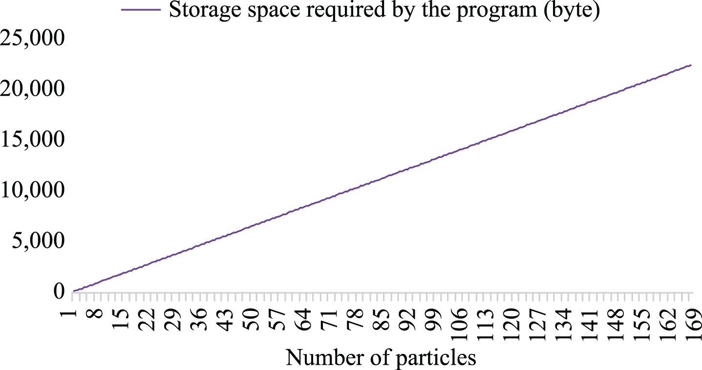
Relationship between number of particles and program storage space.

6.2.2 Particle self-acceleration weight coefficient

Assume that particle _ num = 20, c₂ = 2, w = 1.4. When the value of c₁ varies, the storage space required for the program operation is not affected. Constantly changing the value of c₁ within the interval, we repeated the experiment 250 times for each value of c₁ and recorded the success rate and the running time of the program, as shown in Table 7.

Table 7
Success rate and average running time of the system when the value of c₁ varies

c ₁ Solution success rate Average program running time (ns)

0.01 100.00% 96,442

0.02 100.00% 25,971

0.03 100.00% 23,078

0.04 100.00% 17,976

0.05 100.00% 25,308

⋯ ⋯ ⋯

4.66 100.00% 19,781

4.67 99.60% 80,363

4.68 99.60% 64,019

4.69 98.80% 173,739

4.70 99.60% 59,123

⋯ ⋯ ⋯

9.96 99.20% 84,711

9.97 99.60% 52,054

9.98 100.00% 23,170

9.99 100.00% 23,187

10.00 99.20% 79,000

c ₁	Solution success rate	Average program running time (ns)
0.01	100.00%	96,442
0.02	100.00%	25,971
0.03	100.00%	23,078
0.04	100.00%	17,976
0.05	100.00%	25,308
⋯	⋯	⋯
4.66	100.00%	19,781
4.67	99.60%	80,363
4.68	99.60%	64,019
4.69	98.80%	173,739
4.70	99.60%	59,123
⋯	⋯	⋯
9.96	99.20%	84,711
9.97	99.60%	52,054
9.98	100.00%	23,170
9.99	100.00%	23,187
10.00	99.20%	79,000

The relationship of the particle self-acceleration weight coefficient with the solution success rate and the program running time, given in Table 7, are shown graphically in Figs. 8 and 9, respectively.

Fig. 8

Relationship between c₁ and the solution success rate.

Fig. 9

Relationship between c₁ and the average running time of the program.

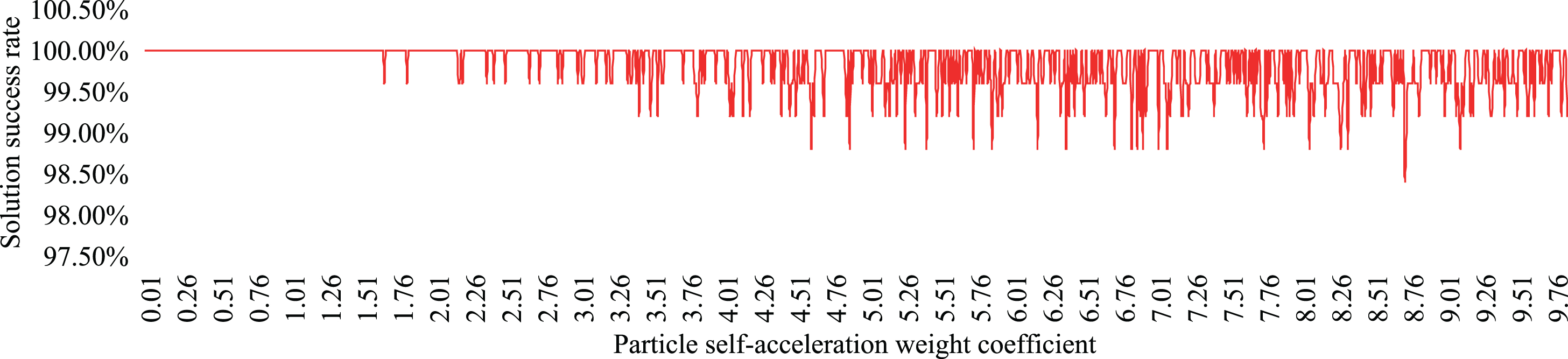
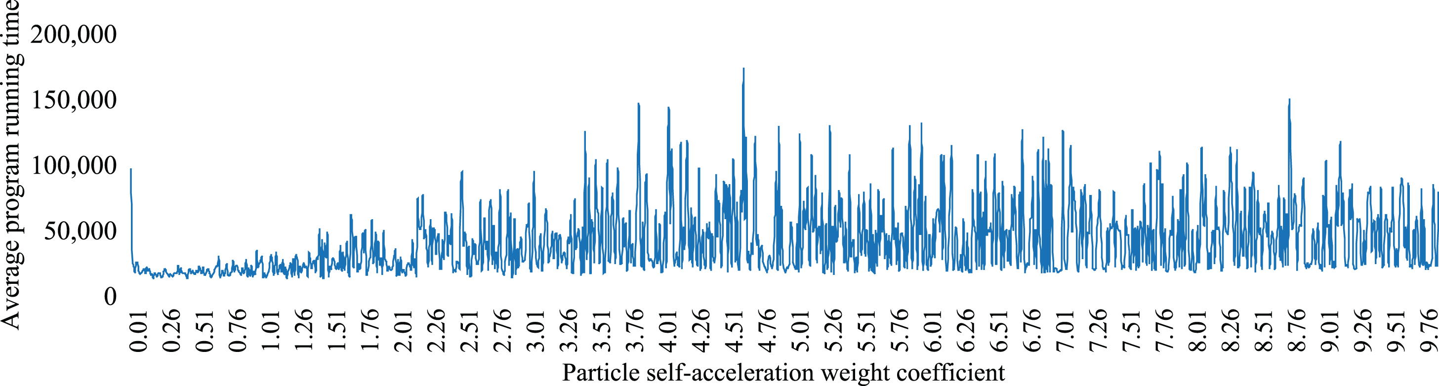
It can be seen from Fig. 8 that when c₁ ∈ [0.01, 1.50], the success rate is stable at 100%, whereas when c₁ > 1.50, the success rate fluctuates to varying degrees, but there are always solutions in multiple experiments. In unsuccessful situations, the solution success rate cannot be stabilized at 100%. It can be seen from Fig. 9 that when c₁ ∈ [0.05, 1.36], the average running time of the system is basically stable between 15 ms and 40 ms, whereas when c₁ > 1.36, the average running time of the system increases to varying degrees, reaching 173 ms at the highest. Considering the system solution success rate and time efficiency comprehensively, the best value range of the particle self-acceleration weight coefficient in this case is c₁ ∈ [0.05, 1.36].

6.2.3 Global acceleration weighting coefficient

Assume that particle _ num = 20, c₁ = 1.2, w = 1.4. When c₂ varies, the storage space required for the program operation is not affected. Constantly changing the value of c₂ within the interval, we repeated the experiment 250 times for each value of c₂ and recorded the success rate of the optimal solution in the experiment and the running time of the program, as shown in Table 8.

Table 8
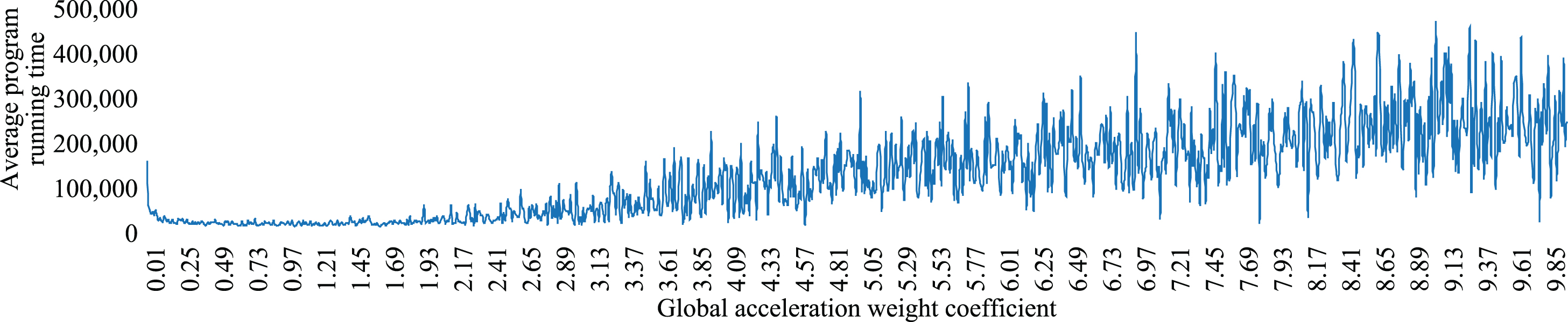
Success rate and average running time of the system when the value of c₂ varies

c ₂ Solution success rate Average program running time (ns)

0.01 100.00% 157,297

0.02 100.00% 61,585

0.03 100.00% 49,160

0.04 100.00% 41,184

0.05 100.00% 46,328

⋯ ⋯ ⋯

4.66 99.60% 141,512

4.67 100.00% 69,789

4.68 99.60% 95,976

4.69 100.00% 73,444

4.70 98.80% 146,781

⋯ ⋯ ⋯

9.96 98.00% 254,036

9.97 98.40% 237,926

9.98 96.40% 387,922

9.99 98.00% 193,058

10.00 98.00% 245,102

c ₂	Solution success rate	Average program running time (ns)
0.01	100.00%	157,297
0.02	100.00%	61,585
0.03	100.00%	49,160
0.04	100.00%	41,184
0.05	100.00%	46,328
⋯	⋯	⋯
4.66	99.60%	141,512
4.67	100.00%	69,789
4.68	99.60%	95,976
4.69	100.00%	73,444
4.70	98.80%	146,781
⋯	⋯	⋯
9.96	98.00%	254,036
9.97	98.40%	237,926
9.98	96.40%	387,922
9.99	98.00%	193,058
10.00	98.00%	245,102

Table 8 shows the relationships between c₂ the solution success rate and program running time, which are also depicted in Figs. 10 and 11, respectively.

Fig. 10

Relationship between c₂ and the solution success rate.

Fig. 11

Relationship between c₂ and the average running time of the program.

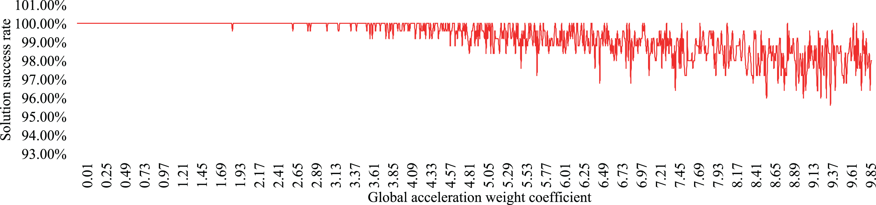
It can be seen from Fig. 10 that when c₂ ∈ [0.01, 1.90], the success rate is stable at 100%, whereas when c₂ > 1.90, the success rate fluctuates to varying degrees, and there are always failures in multiple experiments. In the case of success, the solution success rate cannot be stabilized at 100%. When c₂ = 9.45, there are 11 unsuccessful solutions in 250 experiments. It can be seen from Fig. 11 that when c₂ ∈ [0.05, 1.86], the average running time of the system is basically stable between 13 ms and 35 ms, and that when c₂ > 1.86, the average running time of the system increases to varying degrees. The highest value is 470 ms. Considering the system solution success rate and time efficiency comprehensively, the optimal value range of the global acceleration weight coefficient in this case is c₂ ∈ [0.05, 1.86].

6.2.4 Inertia weighting coefficient of the particle flight

Assume that particle _ num = 20, c₁ = 1.2, c₂ = 1.2. When w varies, the storage space required for the program operation is not affected. Constantly changing the value of w within the interval, we repeated the experiment 250 times for each value of w and recorded the success rate and program running time, as shown in Table 9.

Table 9
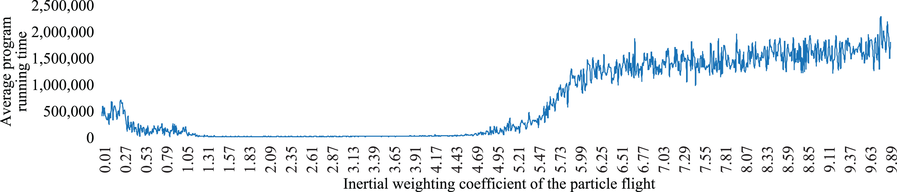
Success rate and average running time of the system when the value of w varies

w Solution success rate Average program running time (ns)

0.01 95.60% 411,495

0.02 92.00% 587,716

0.03 94.80% 407,779

0.04 92.80% 552,637

0.05 94.40% 419,579

⋯ ⋯ ⋯

3.31 100.00% 21,942

3.32 100.00% 19,284

3.33 100.00% 23,375

3.34 100.00% 20,429

3.35 100.00% 16,905

⋯ ⋯ ⋯

9.96 69.60% 2,185, 010

9.97 72.80% 1,986, 520

9.98 74.80% 1,843, 849

9.99 79.60% 1,492, 748

10.00 75.60% 1,794, 040

w	Solution success rate	Average program running time (ns)
0.01	95.60%	411,495
0.02	92.00%	587,716
0.03	94.80%	407,779
0.04	92.80%	552,637
0.05	94.40%	419,579
⋯	⋯	⋯
3.31	100.00%	21,942
3.32	100.00%	19,284
3.33	100.00%	23,375
3.34	100.00%	20,429
3.35	100.00%	16,905
⋯	⋯	⋯
9.96	69.60%	2,185, 010
9.97	72.80%	1,986, 520
9.98	74.80%	1,843, 849
9.99	79.60%	1,492, 748
10.00	75.60%	1,794, 040

Table 9 shows the relationships between w and the solution success rate and program running time, which are also shown in Figs. 12 and 13, respectively.

Fig. 12

Relationship between w and the solution success rate.

Fig. 13

Relationship between w and the average running time of the program.

It can be seen from Fig. 12 that when w ∈ [0.01, 1.20], the success rate of the system solution rises as w increases. When w ∈ [1.20, 4.60], the system success rate is stable at 100%, whereas when w ∈ [4.60, 10.00], it decreases with increasing w, reaching a minimum of 68%. As shown in Fig. 13, when w ∈ [0.01, 1.30], as w increases, the program running time decreases. When w ∈ [1.30, 4.36], the program running time is basically stable between 12 ms and 16 ms, but when w ∈ [4.36, 10.00], the program running time increases with increasing w, reaching 2275 ms, which is 189 times the lowest value. Considering the system solution success rate and system solution time efficiency comprehensively, the optimal value range of w in this case is w ∈ [1.30, 4.36].

Based on the above analysis, the recommended ranges of the parameters of the PSO in this case are particle _ num ∈ [14, 25], c₁ ∈ [0.05, 1.36], c₂ ∈ [0.05, 1.86], and w ∈ [1.30, 4.36].

6.3 Comparative analysis of different algorithms

To demonstrate its effectiveness and rationality, the PSO algorithm proposed in this paper is compared with the Dijkstra algorithm proposed by Broumi in 2017 [53], Bellman algorithm proposed by Broumi in 2019 [55] and ant colony algorithm proposed by Yang in 2020 [58].

6.3.1 Comparison with the Dijkstra algorithm

The adjacency matrix can be established according to the edge weight information of the neutrosophic graph in Table 1: $\begin{matrix} A = \\ [\begin{matrix} 0, {\tilde{N}}_{(AB)}, M, {\tilde{N}}_{(AD)}, {\tilde{N}}_{(AE)}, {\tilde{N}}_{(AF)}, M, M, M, M, M, M, M, M, M, M, M \\ M, 0, {\tilde{N}}_{(BC)}, {\tilde{N}}_{(BD)}, M, M, M, M, M, M, M, M, M, M, M, M, M \\ M, M, 0, {\tilde{N}}_{(CD)}, M, M, {\tilde{N}}_{(CG)}, M, M, M, M, M, M, M, M, M, M \\ M, M, M, 0, M, M, {\tilde{N}}_{(DG)}, {\tilde{N}}_{(DH)}, M, M, M, M, M, M, M, M, M \\ M, M, M, M, 0, M, M, {\tilde{N}}_{(EH)}, {\tilde{N}}_{(EI)}, {\tilde{N}}_{(EJ)}, M, M, M, M, M, M, M \\ M, M, M, M, M, 0, M, M, M, {\tilde{N}}_{(EJ)}, M, M, M, M, M, M, M \\ M, M, M, M, M, M, 0, {\tilde{N}}_{(GH)}, M, M, {\tilde{N}}_{(GK)}, {\tilde{N}}_{(GL)}, M, M, M, M, M \\ M, M, M, M, M, M, M, 0, {\tilde{N}}_{(HI)}, M, M, {\tilde{N}}_{(HL)}, M, M, M, M, M \\ M, M, M, M, M, M, M, M, 0, {\tilde{N}}_{(IJ)}, M, {\tilde{N}}_{(IL)}, {\tilde{N}}_{(IM)}, {\tilde{N}}_{(IN)}, M, M, M \\ M, M, M, M, M, M, M, M, M, 0, M, M, M, {\tilde{N}}_{(JN)}, M, M, M \\ M, M, M, M, M, M, M, M, M, M, 0, {\tilde{N}}_{(KL)}, M, M, {\tilde{N}}_{(KO)}, M, M \\ M, M, M, M, M, M, M, M, M, M, M, 0, {\tilde{N}}_{(LM)}, M, {\tilde{N}}_{(LO)}, M, {\tilde{N}}_{(LQ)} \\ M, M, M, M, M, M, M, M, M, M, M, M, 0, {\tilde{N}}_{(MN)}, M, {\tilde{N}}_{(MP)}, {\tilde{N}}_{(MQ)} \\ M, M, M, M, M, M, M, M, M, M, M, M, M, 0, M, {\tilde{N}}_{(NP)}, M \\ M, M, M, M, M, M, M, M, M, M, M, M, M, M, 0, M, {\tilde{N}}_{(OQ)} \\ M, M, M, M, M, M, M, M, M, M, M, M, M, M, M, 0, {\tilde{N}}_{(PQ)} \\ M, M, M, M, M, M, M, M, M, M, M, M, M, M, M, M, 0 \end{matrix}], \end{matrix}$ where ${\tilde{N}}_{(i, j)}$ represents the neutrosophic edge weight in the interval from node i to node j. Table 1 presents the specific values. M represents an infinite number, indicating that there is no direct edge connection between node i and node j. The steps for using the Dijkstra algorithm to calculate the shortest path from node A to node Q are as follows:

Step 1: Let V be the set of all vertices; S be the set of determined vertices, initially containing only A; L be the set of determined edges, initially empty; and T = V - S be the set of all undetermined vertices. Initially, V = {A, B, C, D, E, F, G, H, I, J, K, L, , M, N, O, P, Q}, S = {A}, T = V - S = {B, C, D, E, F, G, H, I, J, K, L, M, N, O, P, Q}, and L = φ.

Step 2: Find the closest vertex to all elements in set S; that is, find the shortest edge among the edges (A, B), (A, D), (A, E), and (A, F). According to Definition 5, the score functions of the four edges can be calculated as follows: $\begin{matrix} S ({\tilde{N}}_{(AB)}) \\ = \frac{1}{4} \times (\begin{matrix} 2 + 0.1 + 0.4 - 2 \times 0.5 \\ - 2 \times 0.7 - 0.4 - 0.7 \end{matrix}) \\ = - 0.25, \\ S ({\tilde{N}}_{(AD)}) \\ = \frac{1}{4} \times (\begin{matrix} 2 + 0.5 + 0.9 - 2 \times 0.3 \\ - 2 \times 0.6 - 0.1 - 0.3 \end{matrix}) \\ = 0.3, \\ S ({\tilde{N}}_{(AE)}) \\ = \frac{1}{4} \times (\begin{matrix} 2 + 0.4 + 0.8 - 2 \times 0.1 \\ - 2 \times 0.5 - 0.1 - 0.4 \end{matrix}) \\ = 0.375, \\ S ({\tilde{N}}_{(AF)}) \\ = \frac{1}{4} \times (\begin{matrix} 2 + 0.1 + 0.3 - 2 \times 0.2 \\ - 2 \times 0.4 - 0.4 - 0.6 \end{matrix}) \\ = 0.05 . \end{matrix}$

According to Definition 6, $min {{\tilde{N}}_{(AB)}, {\tilde{N}}_{(AD)},$ ${\tilde{N}}_{(AE)}, {\tilde{N}}_{(AF)}} = {\tilde{N}}_{(AF)}$ , i.e., the point closest to A is F, so we update vertex sets S = {A, F} and T = V - S = {B, C, D, E, G, H, I, J, K, L, M, N, O, P, Q} and edge set L = {(AF)}. Because the end point Q ∉ S, it is necessary to return to Step 2 and find all the edges connecting A through the elements in set S. As shown in Fig. 2, the set of edges L₂ = {(AB) , (AD) , (AE) , (AFJ)}. According to Definition 5, the score functions of the four edges can be calculated as follows: $\begin{matrix} S ({\tilde{N}}_{(AB)}) \\ = \frac{1}{4} \times (\begin{matrix} 2 + 0.1 + 0.4 - 2 \times 0.5 \\ - 2 \times 0.7 - 0.4 - 0.7 \end{matrix}) \\ = - 0.25, \\ S ({\tilde{N}}_{(AD)}) \\ = \frac{1}{4} \times (\begin{matrix} 2 + 0.5 + 0.9 - 2 \times 0.3 \\ - 2 \times 0.6 - 0.1 - 0.3 \end{matrix}) \\ = 0.3, \\ S ({\tilde{N}}_{(AE)}) \\ = \frac{1}{4} \times (\begin{matrix} 2 + 0.4 + 0.8 - 2 \times 0.1 \\ - 2 \times 0.5 - 0.1 - 0.4 \end{matrix}) \\ = 0.375, \\ S ({\tilde{N}}_{(AFJ)}) = S ({\tilde{N}}_{(AF)} \oplus {\tilde{N}}_{(FJ)}) \\ = S (\begin{matrix} < [0.1, 0.3], [0.2, 0.4], [0.4, 0.6] > \\ \oplus < [0.2, 0.3], [0.2, 0.6], [0.4, 0.5] > \end{matrix}) \\ = S (< [0.28, 0.51], [0.04, 0.24], [0.16, 0.3] >) \\ = \frac{1}{4} \times (\begin{matrix} 2 + 0.28 + 0.51 - 2 \times 0.04 \\ - 2 \times 0.24 - 0.16 - 0.3 \end{matrix}) \\ = 0.4425 . \end{matrix}$

According to Definition 6, $min {{\tilde{N}}_{(AB)}, {\tilde{N}}_{(AD)},$ ${\tilde{N}}_{(AE)}, {\tilde{N}}_{(AFJ)}} = {\tilde{N}}_{(AB)}$ , i.e., the closest point to A in T is B, so we update S = {A, F, B} and T = V - S = {C, D, E, G, H, I, J, K, L, M, N, O, P, Q} and e L = {(AF) , (AB)}. Because the end point Q ∉ S, Step 2 is repeated continuously until Q is included in S. Finally, S = {A, F, B, D, C, E, J, G, H, N, I, L, P, M, O, K, Q} and $L = {\begin{matrix} (AF), (AB), (AD), (BC), \\ (AE), (FJ), (CG), (DH), \\ (JN), (ET), (GK), (NP), \\ (LM), (LO), (GK), (OQ) \end{matrix}}$ .

Of all the edges in Fig. 2, only the elements in L are retained (Fig. 14).

As shown in Fig. 14, there is only one path A->B->C->G->L->O->Q from A to Q. This finding is consistent with the calculation results of the PSO method proposed in this report, demonstrating the effectiveness of this approach.

Fig. 14

Results calculated using the Dijkstra algorithm.

From the perspective of the computational efficiency of the algorithm, note that each new vertex in S in the Dijkstra algorithm must be compared with an edge other than L. Assuming that the number of vertices in the neutrosophic graph is n, the time cost is O (n²). In contrast, the selected number of particles in the PSO has a linear relationship with the number of vertices. 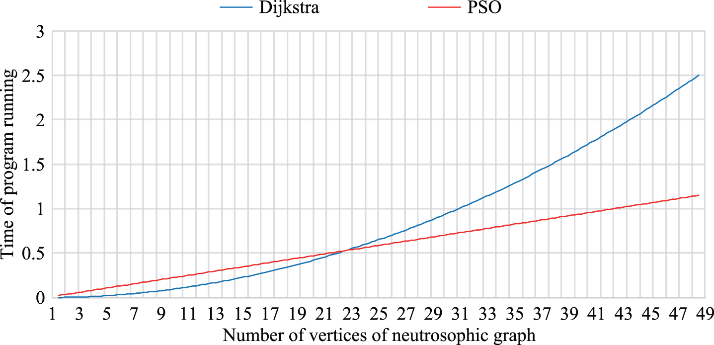According to the data of the case analysis, the number of particles is $\frac{n}{3}$ , number of iterations is approximately 69, and time cost is approximately O (23n). In fact, according to the sensitivity analysis in Section 5.2, when the parameter values are within certain ranges, the PSO can achieve a lower time cost. Figure 15 compares the running times of the PSO and Dijkstra algorithms (assuming that each operation requires time t = 0.001 s).

Fig. 15

Comparison of the running times of the PSO and Dijkstra algorithms.

The abscissa in Fig. 15 represents the number of vertices in the neutrosophic graph, and the ordinate represents the time required for the program to run. From this figure, we can see that when n > 23, PSO has the advantage of a short running time. With increasing n, this advantage increases.

6.3.2 Comparison with the Bellman algorithm

The Bellman algorithm [55] was also used to calculate the calculation examples in this study. Let f (i) represent the score function of the shortest path from A to vertex i and ${\tilde{N}}_{(i, j)}$ represent the neutrosophic edge weight in the interval from node i to node j. We will calculate the shortest path from each vertex to A. $\begin{matrix} f (A) & = 0, \\ f (B) & = min_{i < B} {f (i) \oplus {\tilde{N}}_{(iB)}} \\ = min {f (A) \oplus {\tilde{N}}_{(AB)}} \\ = min {0 \oplus 〈 [0.1, 0.4], [0.5, 0.7], [0.4, 0.7] 〉} \\ = 〈 [0.1, 0.4], [0.5, 0.7], [0.4, 0.7] 〉, \\ f (C) & = min_{i < C} {f (i) \oplus {\tilde{N}}_{(iC)}} \\ = min {f (B) \oplus {\tilde{N}}_{(BC)}} \\ = min {\begin{matrix} 〈 [0.1, 0.4], [0.5, 0.7], [0.4, 0.7] 〉 \\ \oplus 〈 [0.1, 0.4], [0.2, 0.5], [0.4, 0.7] 〉 \end{matrix}} \\ = 〈 [0.19, 0.64], [0.1, 0.35], [0.16, 0.49] 〉, \end{matrix}$

According to this calculation step, we can finally obtain $\begin{matrix} f (Q) = min_{i < Q} {f (i) \oplus {\tilde{N}}_{(iQ)}} \\ = min {\begin{matrix} f (L) \oplus {\tilde{N}}_{(LQ)}, f (M) \oplus {\tilde{N}}_{(MQ)} \\ f (O) \oplus {\tilde{N}}_{(OQ)}, f (P) \oplus {\tilde{N}}_{(PQ)} \end{matrix}} \\ = min {\begin{matrix} 〈 \begin{matrix} , [0.003, 0.126], \\ [0.0064, 0.2058] \end{matrix} 〉 \\ \oplus 〈 [0.6, 0.9], [0.3, 0.5], [0.1, 0.2] 〉, \\ 〈 \begin{matrix} [0.47512, 0.9118], [0.012, 0.0882], \\ [0.00256, 0.12348] \end{matrix} 〉 \\ \oplus 〈 [0.5, 0.8], [0.3, 0.7], [0.2, 0.4] 〉, \\ 〈 \begin{matrix} [0.53344, 0.937], [0.0012, 0.0756], \\ [0.00192, 0.12348] \end{matrix} 〉 \\ \oplus 〈 [0.1, 0.4], [0.2, 0.6], [0.4, 0.7] 〉, \\ 〈 \begin{matrix} [0.4816, 0.8775], [0.0008, 0.0432], \\ [0.0256, 0.168] \end{matrix} 〉 \\ \oplus 〈 [0.2, 0.5], [0.2, 0.5], [0.4, 0.6] 〉 \end{matrix}} \\ = min {\begin{matrix} 〈 \begin{matrix} [0.76675, 0.98741], \\ [0.0009, 0.063], \\ [0.00064, 0.04116] \end{matrix} 〉, \\ 〈 \begin{matrix} [0.73759, 0.98237], \\ [0.00037, 0.06175], \\ [0.00052, 0.0494] \end{matrix} 〉, \\ 〈 \begin{matrix} [0.5801, 0.9622], \\ [0.00024, 0.04536], \\ [0.00077, 0.08644] \end{matrix} 〉, \\ 〈 \begin{matrix} [0.58528, 0.93875], \\ [0.00016, 0.0216], \\ [0.01024, 0.1008] \end{matrix} 〉 \\ = 〈 \begin{matrix} [0.5801, 0.9622], \\ [0.00024, 0.04536], \\ [0.00077, 0.08644] \end{matrix} 〉 . \end{matrix}} \end{matrix}$

Thus, $\begin{matrix} f (Q) = f (O) \oplus {\tilde{N}}_{(OQ)} \\ = f (L) \oplus {\tilde{N}}_{(LO)} \oplus {\tilde{N}}_{(OQ)} \\ = f (G) \oplus {\tilde{N}}_{(GL)} \oplus {\tilde{N}}_{(LO)} \oplus {\tilde{N}}_{(OQ)} \\ = f (C) \oplus {\tilde{N}}_{(CG)} \oplus {\tilde{N}}_{(GL)} \oplus {\tilde{N}}_{(LO)} {\tilde{N}}_{(OQ)} \\ = f (B) \oplus {\tilde{N}}_{(BC)} \oplus {\tilde{N}}_{(CG)} \oplus {\tilde{N}}_{(GL)} {\tilde{N}}_{(LO)} \\ \oplus {\tilde{N}}_{(OQ)} \\ = f (A) \oplus {\tilde{N}}_{(AB)} \oplus {\tilde{N}}_{(BC)} \oplus {\tilde{N}}_{(CG)} {\tilde{N}}_{(GL)} \\ \oplus {\tilde{N}}_{(LO)} \oplus {\tilde{N}}_{(OQ)} \\ = {\tilde{N}}_{(AB)} \oplus {\tilde{N}}_{(BC)} \oplus {\tilde{N}}_{(CG)} \oplus {\tilde{N}}_{(GL)} \\ \oplus {\tilde{N}}_{(LO)} \oplus {\tilde{N}}_{(OQ)} . \end{matrix}$

Therefore, the shortest path P_min sought in this case is A->B->C->G->L->O->Q, and its score function $\begin{matrix} S (P_{min}) = S (f (Q)) \\ = S (\begin{matrix} 〈 \begin{matrix} [0.5801, 0.9622], \\ [0.00024, 0.04536], \\ [0.00077, 0.08644] \end{matrix} 〉 \end{matrix}) \\ = \frac{1}{4} \times (\begin{matrix} 2 + 0.5801 + 0.9622 \\ - 2 \times 0.00024 - 2 \times 0.04536 \\ - 0.00077 - 0.08644 \end{matrix}) \\ = 0.84097 . \end{matrix}$

This finding is consistent with the calculation results of the PSO algorithm proposed in this report, demonstrating the effectiveness of this approach.

From the perspective of computational efficiency, we note that the Bellman algorithm must find the shortest path from all intermediate nodes to the starting point in sequence. Assuming that the number of vertices of the neutrosophic graph is n, the time cost is O (n³). The previous section explained that the time cost of PSO is approximately O (23n). Figure 16 compares of the running times of the PSO and Bellman algorithms (assuming that each operation requires time t = 0.001 s).

Fig. 16

Comparison of the running times of the PSO and Bellman algorithms.

The abscissa in Fig. 16 represents the number of vertices in the neutrosophic graph, and the ordinate represents the time required for the program to run. From this figure, we can see that, as the number of vertices increases, the time required for the Bellman algorithm to run increases significantly faster than that for the particle swarm algorithm. When n > 5, the PSO has the advantage of a smaller running time. As n increases, so does this advantage.

6.3.3 Comparison with the ant colony algorithm

Finally, the ant colony algorithm [58] was applied to the example addressed in this article. The ant colony algorithm, like PSO, is an intelligent algorithm. The number of particles used in the case analysis in this study was 5. For better comparison, we set the number of ants in the ant colony algorithm to five, so that both algorithms would have the same space cost.

Step 1: Initialize the pheromone concentration C_i = 1, i ∈ [1, 176]; number of paths randomly selected in each iteration N = 5; pheromone-volatilization coefficient Δp = 5%; and pheromone-accumulation coefficient of the local optimal solution Δq = 10%.

Step 2: The system randomly selects five paths, P (ADHILOQ), P (ABDHLOQ), P (ADHIMPQ), P (ABCDHLMQ), and P (AEILMNPQ), from A to Q. Calculate the neutrosophic distances of these five paths. $\begin{matrix} {\tilde{N}}_{P (ADHILOQ)} \\ = {\tilde{N}}_{(AD)} \oplus {\tilde{N}}_{(DH)} \oplus {\tilde{N}}_{(HI)} \oplus {\tilde{N}}_{(IL)} \\ \oplus {\tilde{N}}_{(LO)} \oplus {\tilde{N}}_{(OQ)} \\ = 〈 \begin{matrix} [0.9093, 0.99956], \\ [0.00015, 0.04536], \\ [0.000002, 0.00681] \end{matrix} 〉, \\ {\tilde{N}}_{P (ABDHLOQ)} = 〈 \begin{matrix} [0.74601, 0.98561], \\ [0.00049, 0.0741], \\ [0.00049, 0.03529] \end{matrix} 〉, \\ {\tilde{N}}_{P (ADHIMPQ)} = 〈 \begin{matrix} [0.90593, 0.99971], \\ [0.00004, 0.02625], \\ [0.00005, 0.0081] \end{matrix} 〉, \\ {\tilde{N}}_{P (ABCDHLMQ)} = 〈 \begin{matrix} [0.87499, 0.99497], \\ [0.00015, 0.05043], \\ [0.00008, 0.00883] \end{matrix} 〉, \\ {\tilde{N}}_{P (AEILMNPQ)} = 〈 \begin{matrix} [0.88805, 0.99707], \\ [0.00001, 0.00757], \\ [0.00004, 0.00908] \end{matrix} 〉 . \end{matrix}$

Calculate the score function of these five random paths according to Eqs. (5) and (6), and find the minimum value $\begin{matrix} min {\begin{matrix} S ({\tilde{N}}_{P (ADHILOQ)}), S ({\tilde{N}}_{P (ABDHLOQ)}), \\ S ({\tilde{N}}_{P (ADHIMPQ)}), S ({\tilde{N}}_{P (ABCDHLMQ)}), \\ S ({\tilde{N}}_{P (AEILMNPQ)}) \end{matrix}} \\ = S ({\tilde{N}}_{P (ABDHLOQ)}) = 0.88667 . \end{matrix}$

The local optimal solution for the first iteration is P_min[0] = P_(ABDHLOQ).

Step 3: Update the pheromone parameters.

① All pheromones volatilize and are reduced by 5% : C_i = 1 × (1 - 5 %) =95 % , i ∈ [1, 176].

② The local optimal solution accumulates 10% of the pheromone: C_{P
_min[0]} = 0.95 × (1 + 10 %) =1.045.

Step 4: Calculate the ratio of the pheromone of the path P_min[0] to the total pheromone $\begin{matrix} {per}_{(p_{min [0]})} & = \frac{c_{(p_{min [0]})}}{Σ c} = \frac{1.045}{0.95 \times 84 + 1.045} \\ = 0.013, \end{matrix}$ and calculate the number of times P_min[0] is selected next time: $\begin{matrix} N_{p_{min [0]}} = round (N \times {per}_{(p_{min [0]})}) \\ = round (10 \times 0.013) = 0 . \end{matrix}$

That is, there is no need to specify the selected path P_(ABDHLOQ). Then, randomly select another five paths, repeat Steps 2 and 3, and continually obtain the local optimal solutions and update the pheromone. On the 515th pass, we obtain the local optimal solution P_min[514] = P_(ABDHLOQ), the updated pheromone C_P(ABCGLOQ) = 0.02831, and the sum of all path pheromones ΣC = 0.02972. We calculate the ratio of the pheromone of the path P_min[514] to the total pheromone: ${per}_{(p_{min [514]})} = \frac{0.02831}{0.02972} = 0.9525$ . In the next iteration, the number of times P_min[514] is selected is

$\begin{matrix} N_{p_{min [514]}} & = round (N \times {per}_{(p_{min [514]})}) \\ = round (5 \times 0.9525) = 5, \end{matrix}$ i.e., starting from the 516th iteration, the five paths selected are all P_(ABCGLOQ), and there will be no new local optimal solutions afterwards. Thus, the optimal solution converges to P_(ABCGLOQ) and no longer changes. This result is consistent with that of the PSO algorithm.

Figure 17 compares the convergence processes to the local optimal solution for the ant colony algorithm and PSO approach.

Fig. 17

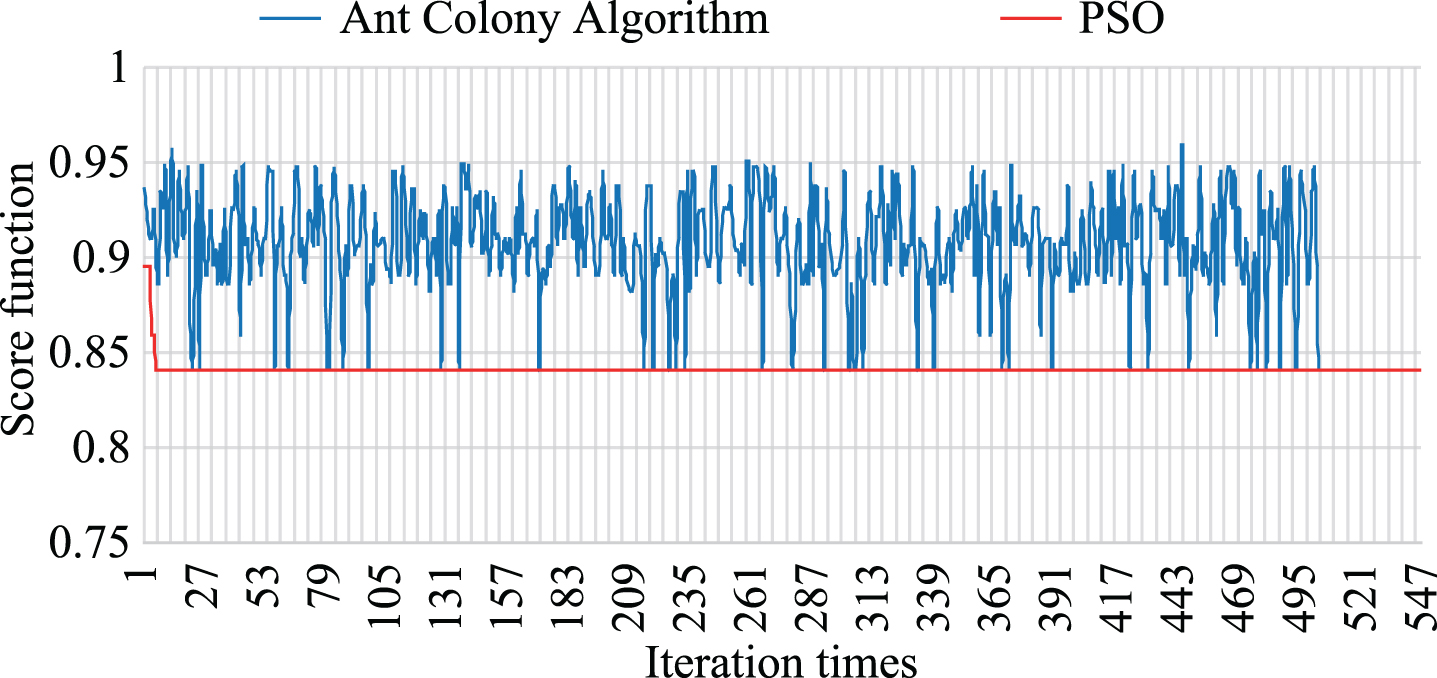
Comparison diagram of the iterative processes of the PSO and ant colony algorithms.

It can be seen from Fig. 17 that the PSO and ant colony algorithms finally converge to the same scoring-function value, i.e., the shortest paths they find are the same. The PSO approach only needs to iterate six times to reach the optimal solution and reaches stable convergence after the 68th iteration. The ant colony algorithm iterates 64 times before the optimal solution appears, after which it undergoes 452 iterations and oscillates at iteration 516. Stable convergence was achieved after two iterations. On the premise that the space cost of the program is consistent, PSO is obviously more efficient than the ant colony algorithm.

From the above comparative analysis, it can be concluded that PSO has the following advantages for solving the SPP of a neutrosophic graph:

PSO is an uncertain algorithm. The uncertainty reflects the biological mechanisms of natural organisms. It does not depend on the strict mathematical nature of the optimization problem. It is thus suitable for the type of environment formed after a typhoon disaster.

PSO is a bio-inspired optimization algorithm based upon multiple agents. The agents in the algorithm cooperate with each other to adapt better to the environment. Distributions can be used when dealing with complex problems with many nodes. Style programming improves the performance of the algorithms.

Compared with traditional methods, PSO is more efficient in solving the SPPs of neutrosophic graphs.

7 Conclusion

In this study, we developed a PSO algorithm for solving the SPP on an interval-valued neutrosophic graph. Firstly, we verified the feasibility of utilizing PSO to solve the problem of typhoon disaster rescue route selection through a case study. Secondly, we conducted a sensitivity analysis of PSO and determined reasonable parameter settings through hundreds of repeated experiments. Finally, we compared the PSO approach with the current mainstream algorithms and proved that PSO is more efficient in solving the SPP of an interval-valued neutrosophic graph. However, the sensitivity analysis also revealed that, when the PSO solves discrete models, it can fall into a local optimal solution when the number of particles is insufficient. In future work, we will further optimize the algorithm to make it even more suitable for solving the SPP of a neutrosophic graph.

Footnotes

Appendix

Table 10 lists the meanings of all notations used in this paper.

Acknowledgments

This work was supported by the National Social Science Foundation of China (No. 17CGL058).

References

Ahuja

R.K.

, Mehlhorn

, Orlin

and Tarjan

R.E.

, Faster algorithms for the shortest path problem, Journal Of The Acm 37 (1990), 213–223. https://doi.org/10.1145/77600.77615

Yang

C.D.

, Lee

D.T.

and Wong

C.K.

, On bends and lengths of rectilinear paths: a graph theoretic approach, International Journal of Computational Geometry & Applications 02 (1992), 61–74. https://doi.org/10.1142/S0218195992000056

Buckley

J.J.

and Jowers

L.J.

, Fuzzy shortest path problem, Studia Fuzziness Soft Computing 222 (2007), 191–193. https://doi.org/10.1007/978-3-540-76290-4_18

Deng

, Chen

, Zhang

and Mahadevan

, Fuzzy Dijkstra algorithm for shortest path problem under uncertain environment, Applied Soft Computing 12 (2012), 1231–1237. https://doi.org/10.1016/j.asoc.2011.11.011

Biswas

S.S.

, Alam

and Doja

M.N.

, An algorithm for extracting intuitionistic fuzzy shortest path in a graph, Applied Computational Intelligence and Soft Computing 2013 (2013), 1–5. https://doi.org/10.1155/2013/970197

and Sotirov

, On solving the quadratic shortest path problem, Informs Journal On Computing 99 (2017), 1–30. https://doi.org/10.1287/ijoc.2018.0861

Zhang

, Song

, Shen

Z.M.

and Wu

, Robust shortest path problem with distributional uncertainty, IEEE Transactions on Intelligent Transportation Systems 19 (2018), 1080–1090. https://doi.org/10.1109/TITS.2017.2709798

Smarandache

, Neutrosophic Set is a Generalization of Intuitionistic Fuzzy Set, Inconsistent Intuitionistic Fuzzy Set (Picture Fuzzy Set, Ternary Fuzzy Set), Pythagorean Fuzzy Set (Atanassov’s Intuitionistic Fuzzy Set of second type), q-Rung Orthopair Fuzzy Set, Spherical Fuzzy Set, and n-HyperSpherical Fuzzy Set, while Neutrosophication is a Generalization of Regret Theory, Grey System Theory, and three-Ways Decision (revisited), J N Theor 29 (2019), 1–35.

Smarandache

, A unifying field in logics, Neutrosophy: Neutrosophic Probability, Set and Logic. American Research Press, Rehoboth, DE, 1999, 7–8.

10.

, Multiple-attribute decision-making method under a single-valued neutrosophic hesitant fuzzy environment, International Journal Of Intelligent Systems 24 (2015), 23–36. https://doi.org/10.1515/jisys-2014-0001

11.

Wang

H.B.

, Interval neutrosophic sets and logic: theory and applications in computing Phoenix, AZ: Wadsworth, 2005, 123–135.

12.

Peng

J.J.

and Wang

J.Q.

, Multi-valued neutrosophic sets and its application in multi-criteria decision-making problems, Neutrosophic Sets & Systems 10 (2015), 3–17.

13.

, Trapezoidal neutrosophic set and its application to multiple attribute decision-making, Neural Computing & Applications 26 (2015), 1157–1166. https://doi.org/10.1007/s00521-014-1787-6

14.

Nancy and Garg

, An improved score function for ranking neutrosophic sets and its application to decision making process, International Journal for Uncertainty Quantification 6 (2016), 377–385. https://doi.org/10.1615/Int.J.UncertaintyQuantification.2016018441

15.

Smarandache

, NeutroAlgebra is a generalization of partial algebra, International Journal of Neutrosophic Science 2 (2020), 8–17.

16.

Mohanta

, Dey

, Pal

, et al., A study of m-polar neutrosophic graph with applications, Journal Of Intelligent & Fuzzy Systems 38 (2020), 4809–4828. https://doi.org/10.3233/JIFS-191520

17.

Son

, Dong

, Son

and Long

, Towards granular calculus of single-valued neutrosophic functions under granular computing, Multimedia Tools And Applications 79 (2020), 16845–16881. https://doi.org/10.1007/s11042-019-7388-8

18.

Tey

, Gan

, Selvachandran

, et al., a novel neutrosophic data analytic hierarchy process for multi-criteria decision making method: A case study in kuala lumpur stock exchange, IEEE Access 7 (2019), 53687–53697. https://doi.org/10.1109/ACCESS.2019.2912913

19.

Dat

, Thong

, Son

, et al., linguistic approaches to interval complex neutrosophic sets in decision making, IEEE Access 7 (2019), 38902–38917. https://doi.org/10.1109/ACCESS.2019.2902841

20.

Edalatpanah

S.A.

, Neutrosophic structured element, Expert Systems With Applications 79 (2020), 1–17. https://doi.org/10.1111/exsy.12542

21.

Ridvan

and Liu

, Maximizing deviation method for neutrosophic multiple attribute decision making with incomplete weight information, Neural Computing & Applications 27 (2016), 2017–2029. https://doi.org/10.1007/s00521-015-1995-8

22.

Deli

, A novel defuzzification method of SV-trapezoidal neutrosophic numbers and multi-attribute decision making: a comparative analysis, Soft Computing 23 (2019), 12529–12545. https://doi.org/10.1007/s00500-019-03803-z

23.

Broumi

, Bakali

, Talea

, Smarandache

and Verma

, Computing minimum spanning tree in interval valued bipolar neutrosophic environment, International Journal of Modeling and Optimization 7 (2017), 300–304. https://doi.org/10.7763/IJMO.2017.V7.602

24.

Peng

and Dai

, Algorithms for interval neutrosophic multiple attribute decision-making based on MABAC, similarity measure, and EDAS, International Journal for Uncertainty Quantification 7 (2017), 395–421. https://doi.org/10.1615/Int.J.UncertaintyQuantification.2017020416

25.

Deli

and Şubaş

, A ranking method of single valued neutrosophic numbers and its applications to multi-attribute decision making problems, International Journal of Machine Learning and Cybernetics 8 (2017), 1309–1322. https://doi.org/10.1007/s13042-016-0505-3

26.

Garg

and Nancy , Non-linear programming method for multi-criteria decision making problems under interval neutrosophic set environment, Applied Intelligence 48 (2018), 2199–2213. https://doi.org/10.1007/s10489-017-1070-5

27.

Faruk

and Khizar

, Some new operations on single-valued neutrosophic matrices and their applications in multi-criteria group decision making, Applied Intelligence 48 (2018), 4594–4614. https://doi.org/10.1007/s10489-018-1226-y

28.

Bolturk

and Kahraman

, A novel interval-valued neutrosophic AHP with cosine similarity measure, Soft Computing 22 (2018), 4941–4958. https://doi.org/10.1007/s00500-018-3140-y

29.

Pramanik

and Mallick

, Distance measure based MADM strategy with interval trapezoidal neutrosophic numbers, Neutrosophic Sets & Systems 19 (2018), 40–46. https://doi.org/10.5281/zenodo.1235165

30.

Deli

, et al., Expansions and reductions on neutrosophic classical soft set S"uleyman Demirel Univ, Journal of Natural and Applied Sciences 22 (2018), 478–486.

31.

Deli

, Operators on single valued trapezoidal neutrosophic numbers and SVTN-group decision making, Neutrosophic Sets & Systems 22 (2018), 131–150. https://digitalrepository.unm.edu/nss_journal/vol22/iss1/11

32.

Deli

and Şubaş

, Some weighted geometric operators with SVTrN-numbers and their application to multi-criteria decision making problems, Journal Of Intelligent & Fuzzy Systems 32 (2017), 291–301. https://doi.org/10.3233/JIFS-151677

33.

Abdel-Basset

, Atef

and Smarandache

, A hybrid neutrosophic multiple criteria group decision making approach for project selection, Cognitive Systems Research 57 (2019), 216–227. https://doi.org/10.1016/j.cogsys.2018.10.023

34.

and Ye

, Similarity measure with indeterminate parameters regarding cubic hesitant neutrosophic numbers and its risk grade assessment approach for prostate cancer patients, Applied Intelligence 50 (2020), 2120–2131.

35.

Schweizer

, Uncertainty: two probabilities for the three states of neutrosophy, International Journal of Neutrosophic Science 2 (2020), 18–26.

36.

Edalatpanah

S.A.

, A direct model for triangular neutrosophic linear programming, International Journal of Neutrosophic Science 1 (2020), 19–28.

37.

Dey

, Le

, Pal

, et al., Fuzzy minimum spanning tree with interval type 2 fuzzy arc length: Formulation and a new genetic algorithm, Soft Computing 3 (2019), 3963–3974. https://doi.org/10.1007/s00500-019-04166-1

38.

Son

, Dong

, Long

, et al., Linear quadratic regulator problem governed by granular neutrosophic fractional differential equations, ISA Transactions 97 (2019), 296–321. https://doi.org/10.1016/j.isatra.2019.08.006

39.

Thong

, Smarandache

, Hoa

, et al., A novel dynamic multi-criteria decision making method based on generalized dynamic interval-valued neutrosophic set, Symmetry 12 (2020), 618–637. https://doi.org/10.3390/sym12040618

40.

Can

, Tu

, Tuan

, et al., A new method to classify malicious domain name using neutrosophic sets in DGA botnet detection, Journal of Intelligent & Fuzzy Systems 38 (2020), 4223–4236. https://doi.org/10.3233/JIFS-190681

41.

Son

, Dong

, Son

, et al., Neutrosophication of statistical data in a study to assess the knowledge, attitude and symptoms on reproductive tract infection among women, Journal of Fuzzy Extension & Applications 2 (2021), 33–40. https://doi.org/10.22105/jfea.2021.272508.1073

42.

Abdel-Basset

, Gamal

, Manogaran

, et al., A novel group decision making model based on neutrosophic sets for heart disease diagnosis, Multimedia Tools And Applications 79 (2020), 9977–10002. https://doi.org/10.1007/s11042-019-07742-7

43.

Jha

, Son

, Kumar

, et al., Neutrosophic image segmentation with dice coefficients, Measurement 134 (2019), 762–772. https://doi.org/10.1016/j.measurement.2018.11.006

44.

Long

, Ali

, Son

, et al., A novel approach for fuzzy clustering based on neutrosophic association matrix, Computers & Industrial Engineering 127 (2019), 687–697. https://doi.org/10.1016/j.cie.2018.11.007

45.

Edalatpanah

S.A.

and Smarandache

, Data envelopment analysis for simplified neutrosophic sets, Neutrosophic Sets & Systems 29 (2019), 215–226. https://digitalrepository.unm.edu/nss_journal/vol29/iss1/17

46.

Yang

, Cai

, Edalatpanah

S.A.

, et al., Triangular single valued neutrosophic data envelopment analysis application to hospital performance measurement, Symmetry 12 (2020), 588–601. https://doi.org/10.3390/sym12040588

47.

Broumi

, et al., Shortest path problemon single valued neutrosophic graphs, presented at the ISNCC-2017, Marrakech, Morocco, 2017, May 16–18.

48.

Yang

, Yan

and Zhao

, Optimal path selection approach for fuzzy reliable shortest path problem, Journal of Intelligent & Fuzzy Systems 32 (2017), 197–205.

49.

Kumar

, Edalatpanah

S.A.

and Mohapatra

, Note on Optimal path selection approach for fuzzy reliable shortest path problem, Journal of Intelligent & Fuzzy Systems 39 (2020), 7653–7656. https://doi.org/10.3233/JIFS-200923

50.

Kumar

, Edalatpanah

S.A.

, Jha

, et al., A multi objective programming approach to solve integer valued neutrosophic shortest path problems, Neutrosophic Sets & Systems 24 (2019), 134–149. https://digitalrepository.unm.edu/nss_journal/vol24/iss1/13

51.

Smarandache

, A Unifying Field in Logics, Neutrosophic Logic, Neutrosophy, Neutrosophic set, Neutrosophic probability, 5th ed. American Research Press, Rehoboth, 2005, 123–135.

52.

Kumar

, et al., Neutrosophic shortest path problem, Neutrosophic Sets & Systems 23 (2018), 5–15.

53.

Broumi

, et al., Application of Dijkstra algorithm for solving interval valued neutrosophic shortest path problem, Computational Intelligence 1 (2017), 1–6.

54.

Tan

, et al., Solving methods for the shortest path problem based on trapezoidal fuzzy neutrosophic numbers, Control and Decision 34 (2019), 851–960.

55.

Broumi

, Dey

, Talea

, Bakali

, Smarandache

, et al., Shortest path problem using Bellman algorithm under neutrosophic environment, Complex & Intelligent Systems 5 (2019), 409–416. https://doi.org/10.1007/s40747-019-0101-8

56.

Chakraborty

, Application of pentagonal neutrosophic number in shortest path problem, International Journal of Neutrosophic Science 3 (2020), 21–28.

57.

Yang

, Li

and Tan

, Shortest path solution of trapezoidal fuzzy neutrosophic graph based on circle-breaking algorithm, Symmetry 12 (2020), 1360–1379. https://doi.org/10.3390/sym12081360

58.

Yang

, Li

and Tan

, Research on the shortest path solution method of interval valued neutrosophic graphs based on the ant colony algorithm, IEEE Access 8 (2020), 88717–88728. https://doi.org/10.1109/ACCESS.2020.2990912

59.

Kennedy

and Eberhart

R.C.

, Particle swarm optimization, Proc IEEE int conf Neural Netw, 1995, 1942–1948.

60.

Poli

, Kennedy

and Blackwell

, Particle swarm optimization, Swarm Intelligence 1 (2007), 33–57. https://doi.org/10.1007/s11721-007-0002-0

61.

Piotrowski

A.P.

, Napiorkowski

J.J.

and A.E, Population size in Particle Swarm Optimization, Swarm and Evolutionary Computation 58 (2020), 100718–100735. https://doi.org/10.1016/j.swevo.2020.100718

62.

Shi

, Liu

, Wu

, et al., Oscillatory Particle Swarm Optimizer, Applied Soft Computing Journal 73 (2018), 316–327. https://doi.org/10.1016/j.asoc.2018.08.037

63.

Xia

, Tang

, Wei

, et al., Dynamic multi-swarm global particle swarm optimization, Computing 102 (2020), 1587–1626. https://doi.org/10.1007/s00607-019-00782-9

Particle swarm optimization for the shortest path problem

Abstract

Keywords

1 Introduction

2 Theoretical basis

2.1 NS

2.2 Interval-valued NNs

4 Interval-valued neutrosophic graph in SPP

5 Shortest path on interval neutrosophic graph via PSO

6.1 Case analysis

Table 3 Main hardware parameters of the experiment Hardware Hardware parameters CPU Intel i7-10700F, 8 cores 16 threads RAM Kingston DDR4 2400 Hz 32 GB Graphics card NVIDIA GTX 1660 super 6 GB Hard disk Kingston SSD 2 TB

6.3.1 Comparison with the Dijkstra algorithm

Footnotes

Appendix

Acknowledgments

References

Table 3
Main hardware parameters of the experiment

Hardware Hardware parameters

CPU Intel i7-10700F, 8 cores 16 threads

RAM Kingston DDR4 2400 Hz 32 GB

Graphics card NVIDIA GTX 1660 super 6 GB

Hard disk Kingston SSD 2 TB