An extended evidential reasoning approach with confidence interval belief structure

Abstract

In Dempster-Shafer theory, belief structure plays a key role, which provides a useful framework for information representation of uncertain variables. Basic Probability Assignment (BPA) is the most important component, which is difficult to be determined due to the uncertainty of information. Generally, there are two ways to get BPA of evidential theory: One is a subjective judgment of the expert’s experience, Interval Belief Structure (IBS) can solve the fuzziness and uncertainty of expert’s judgment. The other is an objective calculation by sampling existing data, in which BPA is viewed as the point estimate. Therefore, one of the contributions of this paper is that the definitions and theories of Confidential Interval Belief Structure (CIBS) is developed to describe BPA in Dempster-Shafer theory, which can give a range of population parameter values and contain more information to deal with the uncertainty and fuzziness of existing data. And then, based on evidential reasoning rule for counter-intuitive behavior, another contribution of this paper is that the extended evidential reasoning approach with CIBS is proposed to obtain the combined belief degree. The proposed method can be flexibly adjusted by appropriate errors and confidence levels, which is the main advantage. Finally, a case of sustainable operation of Shanghai rail transit system to verify the feasibility of proposed method and great performance of the extended method is shown.

Keywords

Evidential reasoning confidence interval belief structures

1 Introduction

From all the databases, the word Evidential Reasoning (ER) first appeared in a paper published in artificial intelligence in [1]. Gordon and Shortliffe proposed Dempster-Shafer (D-S) scheme for evidence aggregation processes in a hypothesis space. Peal shown in [2] that evidential reasoning could be conducted in the same hypothesis space using a Bayesian scheme. Lee analyzed in [3] that the differences of the two scheme. D-S theory is identified as an efficient model to deal with uncertainty information in intelligent systems in [4], which can handle uncertainty more preferable than probability theory in [5]. Nowadays, D-S theory is applied widely in many fields, such as decision-making ([6, 7]), supplier selection ([8, 9]), reliability analysis ([10, 11]), and optimization under uncertain environment ([12, 13]), stochastic modeling ([14]), safety analysis ([15]), stock portfolio selection ([16]), voice activity detection ([17]), financial investment ([18]), supply chain ([19]).

In D-S theory, a piece of evidence is described by a Belief Structure (BS) defined on the power set of the frame of discernment, of which an important component is BPA. Basic probabilities can be assigned to not only singleton propositions, but also any of their subsets. However, due to the uncertainty of Decision Makers’ (DMs) subjective judgments, linguistic ambiguity ([20]) and the lack of information, probability masses assigned to propositions can be uncertain or imprecise ([21]). Group Decision Making (GDM) is characterized as a situation in which individuals collectively make a choice from a set of possible choices ([22 –24]). As the group members participating in the decision-making have differences in knowledge, experience, judgment ability and other personal characteristics, they have different understandings of the pros and cons of the alternatives. In the problem of GDM, belief degrees may be provided by different DMs or experts, although these belief degrees can be synthesized to get a precise point estimate, it will inevitably lead to information loss. To better express the uncertainty of information in D-S theory, the concept of IBS has been proposed ([25]).

IBS, as an extension of BS in D-S theory, the basic probabilities of which is designed by an interval value to better express uncertain and imprecise information ([26]). But in many cases, the basic probability of each evidence is usually objectively calculated by the number of times it occurs through multiple experiments. In this case, IBS ignores the probability law of random variable. The BPA obtained in this way can be viewed as a point estimate. In most cases, each evidence is subject to a certain distribution of the proposition. Therefore, this paper argues that the basic probability of each evidence under propositions can be described by interval estimation instead of point estimation, and the interval estimation of the population samples can be carried out by means of confidence interval. Therefore, by introducing the concept of confidence interval estimation to describe BPA in D-S theory, this paper proposed the concept of CIBS, which extends the IBS.

In the research of D-S theory, combining and normalizing of BS is the most important research directions. As the core of D-S theory, Dempster’s rule plays a key role to extend Bayes’ rule and popularize as the only Evidence Combination Rule (ECR) to combine evidence in D-S theory originally ([27, 28]). However, one concern about Dempster’s rule is that proposition will be ruled out completely when a piece of evidence is not supported a proposition at all. Although it could be supported in some cases, it is generally the case that each piece of evidence has been limited or varying degrees of reliability in supporting and opposing propositions ([29, 30]). Moreover, Dempster’s rule cannot be used when two pieces of evidence are in complete conflict, which has led to a counter-intuitive problem in [31]. In order to solve the problem of counter-intuitive problem, the evidence combination rules have been proposed to take the place of Dempster’s rule for handling the counter-intuitive problem ([32, 33]). At the same time, the methods of combining and normalizing of IBS are also developed ([34, 35]). Sevastianov et al. in [34] developed a new combination approach for the interval evidence combination and normalization; Song et al. in [36] proposed a novel approach to combine evidence based on the operation on intuitionistic fuzzy set. However, these methods cannot be applied to the combination of conflicting interval evidence. Therefore, Zhang et al. developed a new approach to consider the conflicting interval evidence combination in [21]. This method considers both evidence weight and reliability in a more general framework to solve the problems of conflicting IBS combination and normalization. Therefore, by Zhang’s combination method, this paper developed an extended evidential combination approach with CIBS, which can be flexibly adjusted by an appropriate error and confidence level. This has not been considered in the existing studies.

The main contributions of this paper can be summarized as follows:

(1) The concept of CIBS is proposed to characterize BPA obtained from objective calculation.

(2) Three theorems of CIBS are given in this paper, which makes computing easier.

(3) Based on CIBS, the evidence combination method, which is a pair of programming models, is developed to calculate the combined belief degree of pieces of evidence.

(4) The extended evidence reasoning method is applied in the evaluation of the sustainable operation of Shanghai rail transit system. And the implementation steps are as follows:

a. Setting up the indictor system;

b. Collecting data to obtain the belief degree of secondary indicators;

c. Calculating combined belief degree of first-level indicators by the proposed evidence combination method.

The rest of the paper is organized as follows. In Section 2, the introduction of D-S theory, the ER rule for counter-intuitive behavior, the ER rule of IBS and the confidence interval of sample ratio are given briefly. In Section 3, the concept of CIBS is developed and a pair of programming models are proposed to calculate the combined probability masses. And then, a simple example shows the feasibility of proposed programming models. In Section 4, the proposed combined models are applied to the actual problem, and the feasibility is further verified. Finally, different parameters are selected for sensitivity analysis.

2 Preliminaries

In this section, we will briefly introduce the basic concepts of D-S Theory, the ER rule for counter-intuitive behavior, ER rule with IBS and confidence interval of sample ratio.

2.1 D-S Theory

D-S theory is based on a frame of discernment, which composed of a set of mutually exclusive and collectively exhaustive propositions ([27]). And the set denoted by Θ. What’s more, 2^Θ contains all propositions and denoted as 2^Θ = {ϕ, θ₁, . . . , θ_N, {θ₁, θ₂} , . . . , {θ₁, θ_N} , . . . , {θ₁, θ_N-1} , Θ}.

Definition 2.1. ([37, 38]) Suppose Θ = {θ₁, θ₂, , , θ_N} is a set of propositions, with θ_i ⋂ θ_j = ϕ for any i, j ∈ 1, 2, , N and i ≠ j where ϕ is an empty set. Θ is then referred to as a frame of discernment. Suppose T observations were made of an element θ ∈ Θ, each of which resulted in an imprecise (non-specific) measurement given by a set A of values. Let c_i denote the number of occurrences of the set A_i ⊆ Θ, and 2^Θ the set of all subsets of Θ (power set of Θ). A BPA is a function m : 2^Θ → [0, 1], satisfying: ${\begin{matrix} m (ϕ) = 0, \\ \sum_{A \subseteq Θ} m (A) = 1 . \end{matrix}$ (2.1) Note that the domain of BPA, 2^Θ, is different from the domain of a probability density function, which is Θ. This function can be obtained as follows ([27]): $m (A_{i}) = \frac{c_{i}}{T} .$ (2.2) If m (A_i) >0, A_i has occurred at least once, then A_i is called a focal element.

Definition 2.2. ([27]) The belief and plausibility functions are defined as follows: $Bel (A) = \sum_{A_{i} \subseteq A} m (A_{i}), Pl (A) = \sum_{A_{i} ⋂ A \neq ϕ} m (A_{i}) .$ (2.3) With two pieces of independent and fully reliable evidence represented by two BPAs M₁ and M₁ respectively, for any proposition θ ⊆ Θ, Dempster’s rule is given as (2.4):

[m₁ ⊕ m₂] (C) =

{\begin{array}{l} 0, & i f C = ϕ, \\ \frac{\sum_{A_{i} \cap A_{j} = C} m_{1} (A_{i}) m_{2} (A_{j})}{1 - \sum_{A_{i} \cap A_{j} = ϕ} m_{1} (A_{i}) m_{2} (A_{j})}, & i f C \neq ϕ . \end{array}

(2.4)

It is obvious in the above equation that Dempster’s rule provides a process for combining two pieces of non-compensatory evidence, in the sense that if either of them completely opposes a proposition, the proposition will not be supported at all, no matter how strongly it may be supported by the other piece of evidence.

Example 1. ([29]) Let Θ be the frame of discernment with three propositions {H₁, H₂, H₃}. Suppose that two BPAs, m₁ and m₂, are constructed as: $m_{1} (H_{1}) = 0.98, m_{1} (H_{2}) = 0.02, m_{1} (H_{3}) = 0,$ $m_{2} (H_{1}) = 0, m_{2} (H_{2}) = 0.02, m_{2} (H_{3}) = 0.98 .$ Where, we can calculate the degree of conflict

∑_{A_i⋂A_j=ϕ}m₁ (A_i) m₂ (A_j) = 0.9996, and the combined result of evidence m₁ and m₂ as follows: $m_{12}^{'} (H_{1}) = 0, m_{12}^{'} (H_{2}) = 1, m_{12}^{'} (H_{3}) = 0 .$ It is obvious that the proposition H₁ or H₃ will be not supported if either pieces of evidence m₁ and m₂ does not support H₁ or H₃, this result contradicts people’s intuition.

2.2 ER rule for counter-intuitive behavior

To deal with the counter-intuitive problem of Dempster’s rule, based on the review of Shafer’s book ([27]), Yang and Xu proposed a new ER rule to deal with evidence weight in an evidence combination process in [29]. What’s more, due to the difference between evidence importance and reliability, a new ER rule has been developed by Yang and Xu ([29]) to combine evidence with weight and reliability. For example, the importance of an information source in information fusion is expressed by the weight given to the information source by the fusion system designer; the reliability of it indicates its ability to provide a correct assessment or solution to a given problem ([39]).

Definition 2.3. ([29]) Suppose the belief degree β_θ,i represents the likelihood that the evidence e_i is assessed to θ, with 0 ≤ β_θ,i ≤ 1, then e_i is defined as follows: $e_{i} = {(θ, β_{θ, i}), \forall θ \subseteq Θ, \sum_{θ \subseteq Θ} β_{θ, i} = 1} .$ (2.5)

Definition 2.4. ([29]) Suppose ω_i (0 ≤ ω_i ≤ 1) is the weight and r_i (0 ≤ r_i ≤ 1) is the reliability of evidence e_i. The weighted belief degree for e_i defined in the ER rule with evidence weight are defined as (2.6): $m_{θ, i} = {\begin{matrix} 0, & if θ = ϕ, \\ \frac{ω_{i}}{1 + ω_{i} - r_{i}} β_{θ, i}, & if θ \subseteq Θ, θ \neq ϕ, \\ 1 - \frac{ω_{i}}{1 + ω_{i} - r_{i}}, & if θ = P (Θ) . \end{matrix}$ (2.6) In particular, the residual support $1 - \frac{ω_{i}}{1 + ω_{i} - r_{i}}$ of e_i is attached to P (Θ) without the specific proposition Θ. And because θ ⋂ P (Θ) = θ, ∀ θ ⊆ Θ, it can be redistributed to all propositions. And then, the Weighted Belief Distribution (WBD) of e_i, denoted by m_i, is defined as follows: $m_{i} = {(θ, m_{θ, i}), \forall θ \subseteq Θ; (P (Θ), m_{P (Θ), i})} .$ (2.7) What’s more, a special case of WBD id when there is no local ignorance. In this case, WBD is transformed to the following: $m_{i} = {(θ_{n}, \frac{ω_{i}}{1 + ω_{i} - r_{i}} β_{θ_{n}, i}), n = 1, 2, . . ., N;$ $(Θ, {\frac{ω_{i}}{1 + ω_{i} - r_{i}}}_{i} β_{θ_{n}, i}); (P (Θ), (1 - \frac{ω_{i}}{1 + ω_{i} - r_{i}}))} .$ (2.8)

Definition 2.5. ([29]; [21]) Suppose L pieces of independent evidence denoted by Equation (5) and their WBDs are represented by Equations (6) and (7). Let e (i) be the fusion of the first i pieces of discounted evidence, and we have the following formulas for the probability masses: ${\hat{m}}_{θ, e (i)} = [(1 - ω_{i}) m_{θ, e (i - 1)} + m_{P (Θ), e (i - 1)} m_{θ, i}]$ $+ \sum_{B ⋂ C = θ, θ \subseteq Θ} m_{B, e (i - 1)} m_{C, i},$ (2.9) ${\hat{m}}_{P (Θ), e (i)} = (1 - ω_{i}) m_{P (Θ), e (i - 1)},$ (2.10) ${\tilde{m}}_{θ, e (i)} = k \cdot {\hat{m}}_{θ, e (i)}$ $= \frac{{\hat{m}}_{θ, e (i)}}{\sum_{D \subseteq Θ} {\hat{m}}_{D, e (i)} + {\hat{m}}_{P (Θ), e (i)}} (\forall θ \subseteq Θ),$ (2.11) ${\tilde{m}}_{P (Θ), e (i)} = k \cdot {\hat{m}}_{P (Θ), e (i)} =$ $\frac{{\hat{m}}_{P (Θ), e (i)}}{\sum_{D \subseteq Θ} {\hat{m}}_{D, e (i)} + {\hat{m}}_{P (Θ), e (i)}} .$ (2.12) Where $0 \leq {\tilde{m}}_{θ, e (i)}, {\tilde{m}}_{P (Θ), e (i)} \leq 1 .$ And the final combined belief degree is shown as follows: $β_{θ, e (L)} = \frac{{\tilde{m}}_{θ, e (L)}}{1 - {\tilde{m}}_{P (Θ), e (L)}} = \frac{{\hat{m}}_{θ, e (L)}}{\sum_{D \subseteq Θ} {\hat{m}}_{D, e (L)}} (\forall θ \subseteq Θ) .$ (2.13)

Revised Example 1. According to Equations (2.5)–(2.7), we can get

m₁ (H₁) =0.49, m₁ (H₂) =0.01, $m_{1} (H_{3}) = 0, m_{1} (P (Θ)) = 0.5 .$ m₂ (H₁) =0, m₂ (H₂) =0.01, $m_{2} (H_{3}) = 0.49, m_{2} (P (Θ)) = 0.5 .$ According to Equations (2.8)–(2.11), the combined result of m₁ and m₂ is as follows:

$m_{12}^{″} (H_{1}) = 0.327, m_{12}^{″} (H_{2}) = 0.013,$ $m_{12}^{″} (H_{3}) = 0.327, m_{12}^{″} (P (Θ)) = 0.333 .$ According to compare $m_{12}^{″}$ with $m_{12}^{'}$ , the combination result by using ER rule is intuitive.

2.3 ER rule with IBS

To make better use of uncertain and imprecise information, IBS is developed to describe the fuzziness and uncertainty made by experts’ subjective judgments ([25, 26]). Therefore, we will introduce the concepts of IBS based on the literature [40, 41] and [21].

Definition 2.6. ([40]; [21]) Let H = {H₁, H₂, . . . , H_N} be the frame of discernment, F₁, F₂, . . . , F_n be n subsets of H and [a_i, b_i] be n intervals with 0 ≤ a_i ≤ b_i ≤ 1 (i = 1, . . . , n). An IBS is the belief structure on H such that

(1) a_i ≤ m (F_i) ≤ b_i, where 0 ≤ a_i ≤ b_i ≤ 1 (i = 1, . . . , n);

(2) $\sum_{i = 1}^{n} a_{i} \leq 1$ and $\sum_{i = 1}^{n} b_{i} \geq 1$ ;

(3) m (A) =0,∀A ∉ {F₁, F₂, . . . , F_n}.

Definition 2.7. ([41]; [21]) Let m be a valid IBS with interval-valued probability masses a_i ≤ m (F_i) ≤ b_i, i = 1, 2, . . . , n . If $\sum_{j = 1}^{n} b_{j} - (b_{i} - a_{i}) \geq 1$ and $\sum_{j = 1}^{n} a_{j} - (b_{i} - a_{i}) \leq 1, \forall i \in {i \in 1, 2, . . ., n},$ then m is called a normalized IBS.

Definition 2.8. ([40]; [21]) Let m be a normalized IBS on H with interval-valued probability masses a_i ≤ m (F_i) ≤ b_i, i = 1, 2, . . . , n . For A ⊆ H, the belief function (Bel) and the plausibility function (Pl) of A are both the closed intervals defined respectively by ${Bel}_{m} (A) = [{Bel}_{m}^{-} (A), {Bel}_{m}^{+} (A)],$ ${Pl}_{m} (A) = [{Pl}_{m}^{-} (A), {Pl}_{m}^{+} (A)] . (2.14)$ where ${Bel}_{m}^{-} (A) = min \sum_{F_{i} \subseteq A} m (F_{i})$ = max [∑_{F_i⊆A}a_i, (1 - ∑_{F_i⊄A}b_j) ] , (2.15) ${Bel}_{m}^{+} (A) = max \sum_{F_{i} \subseteq A} m (F_{i})$ = min [∑_{F_i⊆A}b_i, (1 - ∑_{F_i⊄A}a_j) ] , (2.16) ${Pl}_{m}^{-} (A) = min \sum_{F_{i} ⋂ A \neq ϕ} m (F_{i})$ = max [∑_{F_i⋂A≠ϕ}a_i, (1 - ∑_{F_i⋂A=ϕ}b_j) ] , (2.17) ${Pl}_{m}^{+} (A) = max \sum_{F_{i} ⋂ A \neq ϕ} m (F_{i})$ = min [∑_{F_i⋂A≠ϕ}b_i, (1 - ∑_{F_i⋂A=ϕ}a_j) ] . (2.18)

Definition 2.9. ([41];[21]) Suppose IBSs m₁ and m₂ are two normalized IBSs, the following pairs of optimization models can be applied to determine the normalized probability mass interval for each proposition. $\begin{matrix} Max / Min β_{θ, e (2)} = \frac{{\tilde{m}}_{θ, e (2)}}{1 - {\tilde{m}}_{P (Θ), e (2)}} \\ s . t . {\hat{m}}_{θ, e (2)} = [(1 - \tilde{ω_{2}}) {\tilde{m}}_{θ, (2 - 1)} + {\tilde{m}}_{P (Θ), e (2 - 1)} {\tilde{m}}_{θ, 2}] \\ + \sum_{B ⋂ C = θ} {\tilde{m}}_{B, e (2 - 1)} {\tilde{m}}_{C, 2}, \forall θ \subseteq Θ, \\ {\hat{m}}_{P (Θ), e (2)} = (1 - \tilde{ω_{2}}) {\tilde{m}}_{P (Θ), e (2 - 1)}, \\ {\tilde{m}}_{θ, e (2)} = {\hat{m}}_{θ, e (2)} / (\sum_{D \subseteq Θ} {\hat{m}}_{D, e (2)} + {\hat{m}}_{P (Θ), e (2)}), \\ {\tilde{m}}_{θ, 1} + {\tilde{m}}_{θ, 2} = 1, \\ {\tilde{m}}_{θ, 1}^{-} \leq {\tilde{m}}_{θ, 1} \leq {\tilde{m}}_{θ, 1}^{+}, {\tilde{m}}_{θ, 2}^{-} \leq {\tilde{m}}_{θ, 2} \leq {\tilde{m}}_{θ, 2}^{+}, \\ \tilde{ω_{2}} = \frac{ω_{2}}{1 + ω_{2} - r_{2}}, 0 \leq r_{2} \leq 1, \\ \tilde{ω_{1}} + \tilde{ω_{2}} = 1, \tilde{ω_{1}} \geq 0, \tilde{ω_{2}} \geq 0 . \end{matrix}$ (2.19)

Example 2. ([21]) Let Θ be the frame of discernment with three propositions {H₁, H₂, H₃}. Suppose that two normalized IBSs, m₁ and m₂, are constructed as: $m_{1} (H_{1}) = [0.98, 0.99], m_{1} (H_{2}) = [0.01, 0.02],$ $m_{1} (H_{3}) = [0, 0];$ $m_{2} (H_{1}) = [0, 0], m_{2} (H_{2}) = [0.01, 0.02],$ $m_{2} (H_{3}) = [0.98, 0.99] .$

The final combined results can be obtained by different methods, which are presented in Table 1.

Table 1

The index system

	m₁₂ =	m₁₂ =	m₁₂ =
	(H₁)	(H₂)	(H₃)
Wang’s method ([42])	[0,0]	[1,1]	[0,0]
Sevastianov’s method ([34])	[0,0]	[0.40,1.60]	[0,0]
Song’s method ([35])	[0,0]	[1,1]	[0,0]
Chen’s method ([41])	[0,0]	[1,1]	[0,0]
Zhang’s method ([21])	[0.327, 0.330]	[0.007, 0.013]	[0.327, 0.330]

2.4 Confidence interval (CI)

Point estimation and interval estimation are two methods of sampling inference. Point estimation is an inferential method without considering sampling error in sampling inference. It is inevitable that there will be errors. Interval estimation is an inference method to estimate the possible range of the total index. When inferring the total index from the sampling index, a certain probability is used to ensure that the error does not exceed a given range.

That is to say, we want to define an interval so that we believe with a high degree of reliability that it contains an unknown population parameter. The degree of reliability is measured in terms of probability, which is called confidence probability or CI.

Definition 2.10. ([43]) Suppose that θ is an unknown parameter, and it exists the interval [θ₁, θ₂], for the given 0 < α < 1, if $P {θ_{1} \leq θ \leq θ_{2}} = 1 - α,$ and then the interval [θ₁, θ₂] is called the CI of θ, and 1 - α is called the confidence level. What’s more, θ₁ and θ₂ are confidence lower limit and confidence upper limit, respectively.

In this paper, we only use the CI estimation of sample ratio.

Definition 2.11. ([43]) Suppose that the sample ratio $\bar{p}$ is a point estimate of the population ratio p. The formula of sample ratio $\bar{p}$ is as follows: $\bar{p} = \frac{x}{T},$ where, x is the number of individuals that have a characteristic, and T denotes sample size.

The sampling distribution of p is the probability distribution of all possible values for the sample ratio $\bar{p}$ . To determine the value of the population ratio p, the following properties of the sampling distribution of sample ratio $\bar{p}$ will be shown.

Definition 2.12. ([43]) Let $\bar{p}$ is the sample ratio and n is the sample size. Let p is the population ratio and the population is infinite. Suppose that np ≥ 5 and n (1 - p) ≥5, the CI of population ratio p is as follows: $[\bar{p} - z_{\frac{α}{2}} \sqrt{\frac{\bar{p} (1 - \bar{p})}{n}}, \bar{p} + z_{\frac{α}{2}} \sqrt{\frac{\bar{p} (1 - \bar{p})}{n}}] .$ (2.20) Where, 1 - α is the confidence level, $z_{\frac{α}{2}}$ denotes the z - value of area α on a standard normal distribution. Next, we further consider what sample size should be selected to estimate the population ratio at a given level of accuracy.

Theorem 2.13 ([43]) Let $\bar{p}$ is the sample ratio and n is the sample size. Let p is the population ratio and the population is infinite. Let E denotes the expected error, and $E = z_{\frac{α}{2}} \sqrt{\frac{p^{*} (1 - p^{*})}{n}} .$ Then, the formula of sample size n is as follows: $n = \frac{z_{\frac{α}{2}}^{2} p^{*} (1 - p^{*})}{E^{2}} .$ (2.21) Where, due to $\bar{p}$ is unknown before sampling, the planned value p^* is defined to replace $\bar{p}$ . From formula (15), the error E is inversely proportional to the sample size n. What’s more, because the bigger p^* (1 - p^*) is, the bigger n is, and the smaller E is. Therefore, when p^* is not sure, p^* = 0.5 is usually taken (From Table 2).

Table 2

The possible values of p^* (1 - p^*)

p ^*	p^* (1 - p^*)
0.1/0.9	0.1*0.9=0.09
0.2/0.8	0.2*0.8=0.16
0.3/0.7	0.3*0.7=0.21
0.4/0.6	0.4*0.6=0.24
0.5	0.5*0.5=0.25	← the maximum value of p^* (1 - p^*)

When p^* = 0.5, the relationships between the sample size n and error E, confidence level 1 - α are shown in Table 3.

Table 3

The sample size n

1 - α\E	0.01	0.02	0.03	0.04	0.05	0.075	0.1
99.9%	27225	6807	3025	1702	1089	484	273
99%	16590	4148	1844	1037	664	296	166
95%	9604	2401	1068	601	385	171	97
90%	6807	1702	757	426	273	122	69

In this paper, we will introduce above concepts to ER method.

3 Extension of ER rule based on CIBS

In the ER theory, the BPA of empty set is 0, the BPA in the whole set represents the global ignorance uncertainty, the BPA over a subclass of a single proposition represents local ignorance uncertainty. If a BPA contains neither the global ignorance uncertainty nor the local ignorance uncertainty, then the BPA function is reduced to the traditional probability function.

In this section, let H = {H₁, H₂, . . . , H_N} be the frame of discernment, F₁, F₂, . . . , F_n be the subsets of H. Let X be the set of samples and T samples are taken from that as observations. Suppose that $m (F_{i}) = \frac{c_{i}}{T} \in$ [0, 1] (i = 1, 2, . . . , n) is defined as the BPA and it is approximately normally distributed, c_i denotes the number of samples that can support F_i in T and $\sum_{i = 1}^{n} c_{i} = T$ , that is $\sum_{i = 1}^{n} m (F_{i}) = 1$ .

Definition 3.1. An confidence interval belief structure (CIBS) is the belief structure on H such that

(1) m^CI (F_i) =

$[max {m (F_{i}) - z_{\frac{α}{2}} \sqrt{\frac{m (F_{i}) (1 - m (F_{i}))}{T}}, 0},$

$min {m (F_{i}) + z_{\frac{α}{2}} \sqrt{\frac{m (F_{i}) (1 - m (F_{i}))}{T}}, 1}];$

(2) m^CI (A) =0, ∀ A ∉ {F₁, F₂, . . . , F_n} .

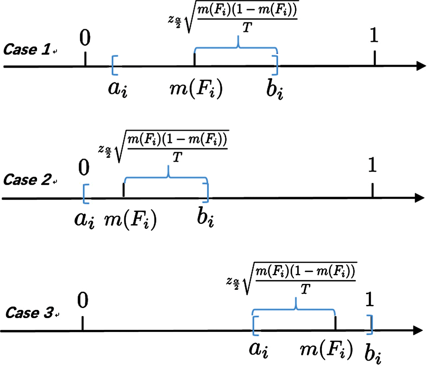
Where, 1 - α is the confidence level, $z_{\frac{α}{2}}$ denotes the z - value of area α on a standard normal distribution. Based on the concept of CIBS, three cases of CIBS can be expressed as follows, which are given in Fig. 1.

Fig. 1

Three cases of CIBS m^CI (F_i) on H.

Case 1:

$m^{CI} (F_{i}) = [m (F_{i}) - z_{\frac{α}{2}} \sqrt{\frac{m (F_{i}) (1 - m (F_{i}))}{T}},$

$m (F_{i}) + z_{\frac{α}{2}} \sqrt{\frac{m (F_{i}) (1 - m (F_{i}))}{T}}]$ ;

Case 2:

$m^{CI} (F_{i}) = [0, m (F_{i}) + z_{\frac{α}{2}} \sqrt{\frac{m (F_{i}) (1 - m (F_{i}))}{T}}]$ ;

Case 3:

$m^{CI} (F_{i}) = [m (F_{i}) - z_{\frac{α}{2}} \sqrt{\frac{m (F_{i}) (1 - m (F_{i}))}{T}}, 1]$ .

Based on Definition 3.1 and Fig. 1, three theorems of CIBS are given as follows. In order to simplify, let $S_{i} = \sqrt{m (F_{i}) (1 - m (F_{i}))}$ (i = 1, 2, . . . , n) and $m^{CI} (F_{i}) = [a_{i}, b_{i}] = [max {m (F_{i}) - \frac{z_{\frac{α}{2}}}{\sqrt{T}} S_{i}, 0},$ $min {m (F_{i}) + \frac{z_{\frac{α}{2}}}{\sqrt{T}} S_{i}, 0}] .$

Theorem 3.1. $\sum_{i = 1}^{n} a_{i} \leq 1$ and $\sum_{i = 1}^{n} b_{i} \geq 1$ .

Proof. Since $\sum_{i = 1}^{n} m (F_{i}) = 1$ and $\frac{z_{\frac{α}{2}}}{\sqrt{T}} \geq 0,$ we have

$\sum_{i = 1}^{n} a_{i} = \sum_{i = 1}^{n} max {m (F_{i}) - \frac{z_{\frac{α}{2}}}{\sqrt{T}} S_{i}, 0}$ $= max {1 - \frac{z_{\frac{α}{2}}}{\sqrt{T}} \sum_{i = 1}^{n} S_{i}, 0} \leq 1;$ $\sum_{i = 1}^{n} b_{i} = \sum_{i = 1}^{n} min {m (F_{i}) + \frac{z_{\frac{α}{2}}}{\sqrt{T}} S_{i}, n}$ $= min {1 + \frac{z_{\frac{α}{2}}}{\sqrt{T}} \sum_{i = 1}^{n} S_{i}, n} \geq 1 .$

This theorem is the condition Of Definition 2.6, which shows that CIBS has the better properties.

Theorem 3.2.

(1) If m (F_i) =0, then m^CI (F_i) = [a_i, b_i] =0;

(2) If m (F_i) =1, then m^CI (F_i) = [a_i, b_i] =1 and m_j≠i (F_j) =0, that is $\underset{j \neq i}{m^{CI}} (F_{j}) = [a_{j}, b_{j}] = 0$ .

Proof. (1) If m (F_i) =0, we have that $a_{i} = max {m (F_{i}) - \frac{z_{\frac{α}{2}}}{\sqrt{T}} S_{i}, 0} = 0,$ $b_{i} = min {m (F_{i}) + \frac{z_{\frac{α}{2}}}{\sqrt{T}} S_{i}, 1} = 0 .$

Thus, m^CI (F_i) = [a_i, b_i] = [0, 0] =0.

(2) If m (F_i) =1, one has $a_{i} = max {m (F_{i}) - \frac{z_{\frac{α}{2}}}{\sqrt{T}} S_{i}, 0} = max {1, 0} = 1,$ $b_{i} = min {m (F_{i}) + \frac{z_{\frac{α}{2}}}{\sqrt{T}} S_{i}, 1} = min {1, 1} = 1 .$ Thus, m^CI (F_i) = [a_i, b_i] = [1, 1] =1.

What’s more, since $\sum_{j = 1}^{n} m (F_{j}) = 1$ and 0 ≤ m (F_j) ≤1 (j = 1, 2, . . . , n) , one has $\sum_{j = 1}^{n} m (F_{j}) - m (F_{i}) = \sum_{j \neq i}^{n} m (F_{j}) = 1 - 1 = 0,$ thus m_j≠i (F_i) =0, that is, $\underset{j \neq i}{m^{CI}} (F_{j}) = [a_{j}, b_{j}] = 0$ .

BS or IBS needs to be standardized of each evidence in the combination of evidences. In fact, CIBS is a special IBS, which is standardized. To proof that, the following two lemmas are given.

Lemma 3.1. If $m (F_{i}) + \frac{z_{\frac{α}{2}}}{\sqrt{T}} S_{i} > 1$ , then $m (F_{i}) - \frac{z_{\frac{α}{2}}}{\sqrt{T}} S_{i} > 0,$ that is $m^{CI} (F_{i}) = [m (F_{i}) - \frac{z_{\frac{α}{2}}}{\sqrt{T}} S_{i}, 1]$ . Where, i = {1, 2, . . . , n}.

Proof. Due to $m (F_{i}) + \frac{z_{\frac{α}{2}}}{\sqrt{T}} S_{i} > 1 (i \in {1, 2, . . ., n})$ , it is obvious that $\frac{z_{\frac{α}{2}}}{\sqrt{T}} S_{i} > 1 - m (F_{i}),$ let’s multiply both sides of this inequality by $\frac{\sqrt{T}}{z_{\frac{α}{2}}} \sqrt{\frac{m (F_{i})}{1 - m (F_{i})}} > 0$ , one has $m (F_{i}) > \frac{\sqrt{T}}{z_{\frac{α}{2}}} S_{i} .$

In general, based on the actual situation, $0 < \frac{z_{\frac{α}{2}}^{2}}{T} < 1$ , and then $m (F_{i}) > \frac{z_{\frac{α}{2}}^{2}}{T} \cdot \frac{\sqrt{T}}{z_{\frac{α}{2}}} \sqrt{m (F_{i}) (1 - m (F_{i}))} = \frac{z_{\frac{α}{2}}}{\sqrt{T}} S_{i} .$ Thus, we can get that $m (F_{i}) - \frac{z_{\frac{α}{2}}}{\sqrt{T}} S_{i} > 0,$ that is $m^{CI} (F_{i}) = [m (F_{i}) - \frac{z_{\frac{α}{2}}}{\sqrt{T}} S_{i}, 1] .$

Lemma 3.2. $\sum_{j = 1, j \neq k}^{n} (S_{j}) - S_{k} \geq 0 (k = 1, 2, . . ., n),$ where $S_{j} = \sqrt{m (F_{j}) (1 - m (F_{j}))}$ .

Proof. It follows from m (F_j) ∈ [0, 1] and $\sum_{j = 1}^{n} m (F_{j}) = 1$ that 0 ≤ m (F_j) (1 - m (F_j)) ≤1 (j = 1, 2, . . . , n) , and $0 \leq m (F_{k}) = 1 - \sum_{j = 1, j \neq k}^{n} m (F_{j}) \leq 1, (\forall k = 1, 2, . . ., n) .$ What’s more, we can find that

$[\sum_{j = 1, j \neq k}^{n} (S_{j})]^{2} = [\sum_{j = 1, j \neq k}^{n} (\sqrt{m (F_{j}) (1 - m (F_{j}))})]^{2}$ $\geq \sum_{j = 1, j \neq k}^{n} [m (F_{j}) (1 - m (F_{j}))] .$ Thus, to get the conclusion, we could prove that

$\sum_{j = 1, j \neq k}^{n} [m (F_{j}) (1 - m (F_{j}))] \geq S_{k}$ $= (1 - \sum_{j = 1, j \neq k}^{n} m (F_{j})) \cdot \sum_{j = 1, j \neq k}^{n} m (F_{j}) .$ (3.6) Next, we will prove the formula of (3.6) by mathematical induction.

(1) For n = 2, it is clear that m (F₁) (1 - m (F₁)) = m (F₂) (1 - m (F₂)), the formula of (3.6) holds.

(2) Suppose that (3.7) holds for some n - 1 >2.

(3) Consider the case of n, for all k ∈ {1, 2, . . . , n - 1}, by induction, the formula of (3.7) holds for all n. And we can get that

$\sum_{j = 1, j \neq k}^{n} [m (F_{j}) (1 - m (F_{j}))]$ $= \sum_{j = 1, j \neq k}^{n - 1} + m (F_{n}) (1 - m (F_{n}))$ $\geq \sum_{j = 1, j \neq k}^{n} m (F_{j}) - [\sum_{j = 1, j \neq k}^{n} m (F_{j})]^{2}$ $= (1 - \sum_{j = 1, j \neq k}^{n} m (F_{j})) \cdot \sum_{j = 1, j \neq k}^{n} m (F_{j});$ for k = n,

$\sum_{j = 1, j \neq k}^{n} [m (F_{j}) (1 - m (F_{j}))]$ $= \sum_{j = 1}^{n - 1} [m (F_{j}) (1 - m (F_{j}))] \geq \sum_{j = 1}^{n - 1} m (F_{j})$ $- [\sum_{j = 1}^{n - 1} m^{2} (F_{j}) + \sum_{a = 1}^{n - 1} \sum_{b = 1, b \neq a}^{n - 1} m (F_{a}) m (F_{b})]$ $= (1 - \sum_{j = 1, j \neq k}^{n} m (F_{j})) \cdot \sum_{j = 1, j \neq k}^{n} m (F_{j}) .$ therefore, $\sum_{j = 1, j \neq k}^{n} S_{j} = \sum_{j = 1, j \neq k}^{n} [\sqrt{m (F_{j}) (1 - m (F_{j}))}] \geq$ $(1 - \sum_{j = 1, j \neq k}^{n} m (F_{j})) \cdot \sum_{j = 1, j \neq k}^{n} m (F_{j}) (\forall k = 1, 2, . . ., n),$ that is, for all k = 1, 2, . . . , n, $\sum_{j = 1, j \neq k}^{n} S_{j} = \sum_{j = 1, j \neq k}^{n} (\sqrt{m (F_{j}) (1 - m (F_{j}))})$ $\geq \sqrt{(1 - \sum_{j = 1, j \neq k}^{n} m (F_{j})) \cdot \sum_{j = 1, j \neq k}^{n} m (F_{j})}$ $= S_{k} .$

Next, based on above two lemmas, the normalized m^CI is proved as follows:

Theorem 3.3. m^CI is a normalized CIBS.

Proof. Since $a_{i} = max {m (F_{i}) - \frac{z_{\frac{α}{2}}}{\sqrt{T}} S_{i}, 0},$ $b_{i} = min {m (F_{i}) + \frac{z_{\frac{α}{2}}}{\sqrt{T}} S_{i}, 1},$ (3.7) and then, $\sum_{i = 1}^{n} a_{i} = 1 - \frac{z_{\frac{α}{2}}}{\sqrt{T}} \sum_{i = 1}^{n} S_{i},$ $\sum_{i = 1}^{n} b_{i} = 1 + \frac{z_{\frac{α}{2}}}{\sqrt{T}} \sum_{i = 1}^{n} S_{i} .$ (3.8)

(a). For some i ∈ {1, 2, . . . , n}, m (F_i) =1. It follows from (3.7)-(3.8) that

$\sum_{j = 1}^{n} b_{j} - (b_{i} - a_{i}) = \sum_{j = 1}^{n} b_{j} \geq 1,$ $\sum_{j = 1}^{n} a_{j} + (b_{i} - a_{i}) = \sum_{j = 1}^{n} a_{j} \leq 1, \forall i \in {1, 2, . ., n} .$

(b). For all i ∈ {1, 2, . . . , n}, m (F_i) ≠1 . Firstly, we have that $b_{i} - a_{i} = min {m (F_{i}) + \frac{z_{\frac{α}{2}} S_{i}}{\sqrt{T}}, 1} - max {m (F_{i}) - \frac{z_{\frac{α}{2}} S_{i}}{\sqrt{T}}, 0} .$

Based on Lemma 1, there are three results for b_i - a_i.

(b1) If $m (F_{i}) + \frac{z_{\frac{α}{2}}}{\sqrt{T}} S_{i} > 1$ , then $m (F_{i}) - \frac{z_{\frac{α}{2}}}{\sqrt{T}} S_{i} > 0,$ and $b_{i} - a_{i} = 1 - m (F_{i}) + \frac{z_{\frac{α}{2}}}{\sqrt{T}} S_{i} .$

It follows from Lemma 2 and $0 < \frac{z_{\frac{α}{2}}}{\sqrt{T}} < 1$ that

$\sum_{j = 1}^{n} b_{j} - (b_{i} - a_{i})$ $= 1 + \frac{z_{\frac{α}{2}}}{\sqrt{T}} \sum_{j = 1}^{n} S_{j} - (1 - m (F_{i}) + \frac{z_{\frac{α}{2}}}{\sqrt{T}} S_{i})$ $\geq 1 + \frac{z_{\frac{α}{2}}}{\sqrt{T}} \sum_{j \neq i} S_{j} - \frac{z_{\frac{α}{2}}}{\sqrt{T}} S_{i}$ $= 1 + \frac{z_{\frac{α}{2}}}{\sqrt{T}} (\sum_{j \neq i} S_{j} - S_{i}) \geq 1;$ Based on that, it is obvious that $b_{i} - a_{i} \leq \sum_{j = 1}^{n} b_{j} - 1$ and $\sum_{j = 1}^{n} a_{j} + (b_{i} - a_{i}) \leq \sum_{j = 1}^{n} a_{j} + \sum_{j = 1}^{n} b_{j} - 1$ $= (1 - \frac{z_{\frac{α}{2}}}{\sqrt{T}} \sum_{i = 1}^{n} S_{i}) + (1 + \frac{z_{\frac{α}{2}}}{\sqrt{T}} \sum_{i = 1}^{n} S_{i}) - 1 = 1 .$

(b2) If $m (F_{i}) + \frac{z_{\frac{α}{2}}}{\sqrt{T}} S_{i} < 1$ and $0 < m (F_{i}) - \frac{z_{\frac{α}{2}}}{\sqrt{T}} S_{i} < 1,$ then $b_{i} - a_{i} = 2 \frac{z_{\frac{α}{2}}}{\sqrt{T}} S_{i} .$

It follows from Lemma 2 and $0 < \frac{z_{\frac{α}{2}}}{\sqrt{T}} < 1$ that

$\sum_{j = 1}^{n} b_{j} - (b_{i} - a_{i}) = 1 + \frac{z_{\frac{α}{2}}}{\sqrt{T}} \sum_{j = 1}^{n} S_{j} - 2 \frac{z_{\frac{α}{2}}}{\sqrt{T}} S_{i}$ $= 1 + \frac{z_{\frac{α}{2}}}{\sqrt{T}} (\sum_{j \neq i} S_{j} - S_{i}) \geq 1;$ It is obvious that $\sum_{j = 1}^{n} a_{j} + (b_{i} - a_{i}) \leq 1 .$

(b3) If $m (F_{i}) + \frac{z_{\frac{α}{2}}}{\sqrt{T}} S_{i} < 1$ and $m (F_{i}) - \frac{z_{\frac{α}{2}}}{\sqrt{T}} S_{i} < 0,$ then $b_{i} - a_{i} = m (F_{i}) + \frac{z_{\frac{α}{2}}}{\sqrt{T}} S_{i} .$

It follows from Lemma 2 and $0 < \frac{z_{\frac{α}{2}}}{\sqrt{T}} < 1$ that

$\sum_{j = 1}^{n} b_{j} - (b_{i} - a_{i})$ $= 1 + \frac{z_{\frac{α}{2}}}{\sqrt{T}} \sum_{j = 1}^{n} S_{j} - (m (F_{i}) + \frac{z_{\frac{α}{2}}}{\sqrt{T}} S_{i})$ $\geq 1 + \frac{z_{\frac{α}{2}}}{\sqrt{T}} \sum_{j \neq i} S_{j} - \frac{z_{\frac{α}{2}}}{\sqrt{T}} S_{i}$ $= 1 + \frac{z_{\frac{α}{2}}}{\sqrt{T}} (\sum_{j \neq i} S_{j} - S_{i}) \geq 1 .$ It is obvious that $\sum_{j = 1}^{n} a_{j} + (b_{i} - a_{i}) \leq 1 .$

From above results, in any case, let m^CI (F_i) = [a_i, b_i] (i = 1, 2, . . . , n), which is satisfy $\sum_{j = 1}^{n} b_{j} - (b_{i} - a_{i}) \geq 1$ and $\sum_{j = 1}^{n} a_{j} + (b_{i} - a_{i}) \leq 1$ . Therefore, m^CI is a normalized CIBS.

Definition 3.2. Let m^CI be a CIBS on H with CI-value probability masses $max {m (F_{i}) - \frac{z_{\frac{α}{2}}}{\sqrt{T}} S_{i}, 0} \leq m^{CI} (F_{i}) \leq min {m (F_{i}) + \frac{z_{\frac{α}{2}}}{\sqrt{T}} S_{i}, 0} (i = 1, 2, . . ., n)$ , where $S_{i} = \sqrt{(1 - m (F_{i}))} \cdot \sqrt{m (F_{i})}$ . For A ⊆ H, the belief function (Bel) and the plausibility function (PL) of A are defined respectively as follows:

${Bel}_{m} (A) = [{Bel}_{m}^{-} (A), {Bel}_{m}^{+} (A)],$

${Pl}_{m} (A) = [{Pl}_{m}^{-} (A), {Pl}_{m}^{+} (A)] . (3.1)$

Let $a_{i} = max {m (F_{i}) - \frac{z_{\frac{α}{2}}}{\sqrt{T}} S_{i}, 0}, b_{i} = min {m (F_{i}) + \frac{z_{\frac{α}{2}}}{\sqrt{T}} S_{i}, 0},$ where

${Bel}_{m}^{-} (A) = min \sum_{F_{i} \subseteq A} m (F_{i})$ $= max [\sum_{F_{i} \subseteq A} a_{i}, (1 - \sum_{F_{i} ⊄ A} b_{j})],$ (3.2) ${Bel}_{m}^{+} (A) = max \sum_{F_{i} \subseteq A} m (F_{i})$ $= min [\sum_{F_{i} \subseteq A} b_{i}, (1 - \sum_{F_{i} ⊄ A} a_{j})],$ (3.3) ${Pl}_{m}^{-} (A) = min \sum_{F_{i} ⋂ A \neq ϕ} m (F_{i})$ $= max [\sum_{F_{i} ⋂ A \neq ϕ} a_{i}, (1 - \sum_{F_{i} ⋂ A = ϕ} b_{j})],$ (3.4) ${Pl}_{m}^{+} (A) = max \sum_{F_{i} ⋂ A \neq ϕ} m (F_{i})$ $= min [\sum_{F_{i} ⋂ A \neq ϕ} b_{i}, (1 - \sum_{F_{i} ⋂ A = ϕ} a_{j})],$ (3.5)

Definition 3.3. Let m^CI (F_i) = [a_i, b_i], which follows the interval operation rules below:

(1) Addition: m^CI (F_i) + m^CI (F_j) = [a_i + a_j, b_i + b_j];

(2) Subtraction: m^CI (F_i) - m^CI (F_j) = [a_i - a_j, b_i - b_j];

(3) Multiplication: m^CI (F_i) × m^CI (F_j) = [a_i × a_j, b_i × b_j];

(4) Division: m^CI (F_i) ÷ m^CI (F_j) = [a_i ÷ b_j, a_j ÷ b_i].

The interval operation above applies only to one piece of evidence, where the interval operation is between different propositions. Subsequently, based on the ER rule for counter-intuitive behavior, the pair of programming models to calculate the combined probability masses of two pieces of CI evidence.

Definition 3.4. Suppose L pieces of independent evidence are described by (2.5). Let e (i) denoted the combination of the first i pieces of evidence. The final combined belief degree can be obtained by the following pairs of optimization models: $\begin{matrix} Max / Min β_{θ, e (i)} = \frac{{\tilde{m}}_{θ, e (i)}}{1 - {\tilde{m}}_{P (Θ), e (i)}} \\ s . t . {\hat{m}}_{θ, e (i)} = [(1 - \frac{ω_{i}}{1 + ω_{i} - r_{i}}) {\tilde{m}}_{θ, (i - 1)} \\ + {\tilde{m}}_{P (Θ), e (i - 1)} {\tilde{m}}_{θ, i}] + \sum_{B ⋂ C = θ} {\tilde{m}}_{B, e (i - 1)} {\tilde{m}}_{C, i}, \\ {\hat{m}}_{P (Θ), e (i)} = (1 - \frac{ω_{i}}{1 + ω_{i} - r_{i}}) {\tilde{m}}_{P (Θ), e (i - 1)}, \\ {\tilde{m}}_{θ, e (i)} = {\hat{m}}_{θ, e (i)} / (\sum_{D \subseteq Θ} {\hat{m}}_{D, e (i)} + {\hat{m}}_{P (Θ), e (i)}), \\ {\tilde{m}}_{θ, i} = \frac{ω_{i}}{1 + ω_{i} - r_{i}} m_{θ, i}^{CI}, \\ m_{θ, i}^{CI} \geq max {m_{θ, i} - \frac{z_{\frac{α}{2}}}{\sqrt{t_{i}}} S_{i}, 0}, \\ m_{θ, i}^{CI} \leq min {m_{θ, i} + \frac{z_{\frac{α}{2}}}{\sqrt{t_{i}}} S_{i}, 1}, \\ \sum_{θ \subseteq Θ} m_{θ, i}^{CI} = 1, i = 1, 2, . . ., n, \\ \sum_{i} \frac{ω_{i}}{1 + ω_{i} - r_{i}} = 1, \frac{ω_{i}}{1 + ω_{i} - r_{i}} \geq 0, 0 \leq r_{i} \leq 1 . \end{matrix}$ 3.9

Where, m_θ,e(1) = m_θ,1 and m_P(Θ),e(1) = m_P(Θ),1. The objective functions of the above models indicate the respective maximum and minimum final combined belief degree with respect to proposition θ by n pieces of evidence based on e (i). Unlike the literature Definition 2.9, m^CI is normalized and there is no need to standardize it before we solve the pair of models.

To illustrate the implementation process of (3.9), we re-examine the example in [21]:

From the literature [21], the belief degree denoted by a single number (Example 1). In this paper, each belief degree in [21] is seen as a point estimation, which is modified into the following example (Example 3).

Example 3. ([21]) Let Θ be the frame of discernment with three propositions {H₁, H₂, H₃}. Suppose that there are two evidences, $m_{1} (H_{i}) = \frac{c_{i}}{t_{1}}$ and $m_{2} (H_{i}) = \frac{c_{i}}{t_{2}} (i = 1, 2, 3)$ are two belief structures on Θ respectively and it is approximately normally distributed. Where, t₁ and t₂ respectively denote the sample number of two evidences, c_i denotes the number of samples that can support F_i in t₁ or t₂. Two belief degree m₁ and m₂ are constructed as: $m_{1} (H_{1}) = \frac{c_{1}}{t_{1}} = 0.98, m_{1} (H_{2}) = \frac{c_{2}}{t_{1}} = 0.02,$ $m_{1} (H_{3}) = \frac{c_{3}}{t_{1}} = 0 .$ $m_{2} (H_{1}) = \frac{c_{1}}{t_{2}} = 0, m_{2} (H_{2}) = \frac{c_{2}}{t_{2}} = 0.02,$ $m_{2} (H_{3}) = \frac{c_{3}}{t_{2}} = 0.98 .$

Let $m_{1}^{CI}$ and $m_{2}^{CI}$ are CIBSs. Suppose that $m_{1}^{CI}$ and $m_{2}^{CI}$ are infinite, by Definition 8, we can obtain that:

$m_{1}^{CI} (H_{1}) = [max {0.98 - z_{\frac{α}{2}} \sqrt{\frac{0.98 (1 - 0.98)}{t_{1}}}, 0},$

$min {0.98 + z_{\frac{α}{2}} \sqrt{\frac{0.98 (1 - 0.98)}{t_{1}}}, 1}];$

$m_{1}^{CI} (H_{2}) = [max {0.02 - z_{\frac{α}{2}} \sqrt{\frac{0.02 (1 - 0.02)}{t_{1}}}, 0},$

$min {0.02 + z_{\frac{α}{2}} \sqrt{\frac{0.02 (1 - 0.02)}{t_{1}}}, 1}];$

$m_{2}^{CI} (H_{2}) = [max {0.02 - z_{\frac{α}{2}} \sqrt{\frac{0.02 (1 - 0.02)}{t_{2}}}, 0},$

$min {0.02 + z_{\frac{α}{2}} \sqrt{\frac{0.02 (1 - 0.02)}{t_{2}}}, 1}];$

$m_{2}^{CI} (H_{3}) = [max {0.98 - z_{\frac{α}{2}} \sqrt{\frac{0.98 (1 - 0.98)}{t_{2}}}, 0},$

$min {0.98 + z_{\frac{α}{2}} \sqrt{\frac{0.98 (1 - 0.98)}{t_{2}}}, 1}];$ $m_{1}^{CI} (H_{3}) = m_{2}^{CI} (H_{1}) = 0 .$

Next, the different confidence level 1 - α and the error E will be given, and the sample size t₁ and t₂ will be determined by Table 3. For example, suppose their confidence level and the error are given by 1 - α = 99.9% and E = 0.01 respectively, and their sample size by t₁ = t₂ = 27225; suppose confidence level and the error are given by 1 - α = 99% and E = 0.02 respectively, and their sample size by t₁ = t₂ = 4148, etc.

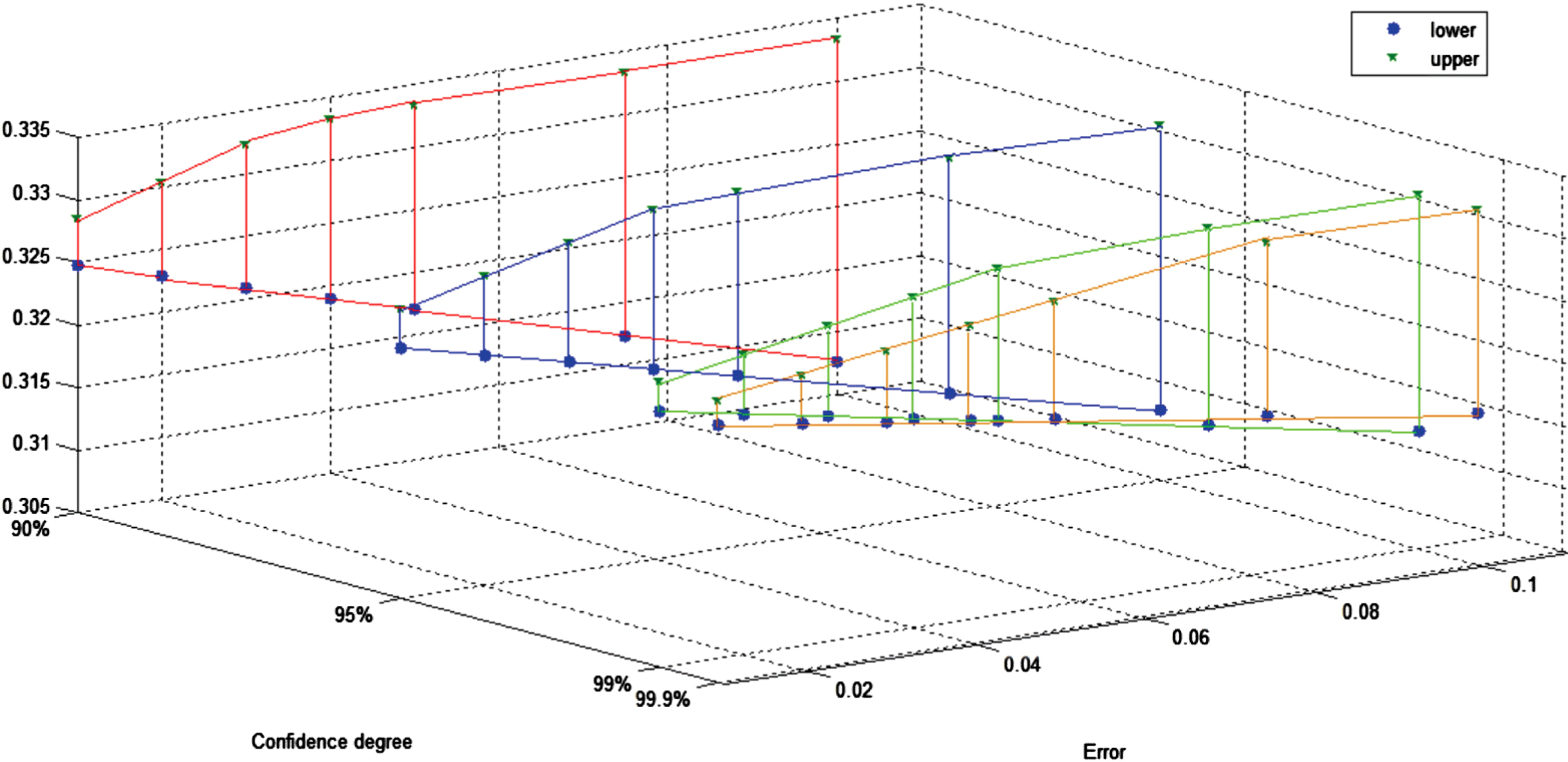
When the sample size t₁, t₂ and confidence level 1 - α are different, the error E are different. Therefore, the sample size can be taken according to the tolerance error E. Let t₁ = t₂, based on Table 3, the different results can be shown in Table 4. And then, the figures of $m_{12}^{CI}$ by different error E and confidence level 1 - α are shown in Figs. 2 and 3. In Fig. 2, the red line denotes the combined CI belief degree when the confidence level 1 - α = 90%; the blue line denotes that when 1 - α = 95%; the green line denotes that when 1 - α = 99%; the yellow line denotes that when 1 - α = 99.9%.

Table 4

The combined belief degree m₁₂

1 - α\E		99.9%			99%			95%			90%
		m₁₂ (H₁)	m₁₂ (H₂)	m₁₂ (H₃)	m₁₂ (H₁)	m₁₂ (H₂)	m₁₂ (H₃)	m₁₂ (H₁)	m₁₂ (H₂)	m₁₂ (H₃)	m₁₂ (H₁)	m₁₂ (H₂)	m₁₂ (H₃)
0.01	min	0.3257	0.0116	0.3257	0.3254	0.0110	0.3254	0.3250	0.0103	0.3250	0.3247	0.0097	0.3247
	max	0.3276	0.0154	0.3276	0.3278	0.0159	0.3278	0.3282	0.0167	0.3282	0.3285	0.0173	0.3285
0.02	min	0.3247	0.0097	0.3247	0.3242	0.0086	0.3242	0.3234	0.0071	0.3234	0.3228	0.0059	0.3228
	max	0.3285	0.0173	0.3285	0.3290	0.0184	0.3290	0.3298	0.0199	0.3298	0.3304	0.0211	0.3304
0.03	min	0.3238	0.0078	0.3238	0.3230	0.0062	0.3230	0.3218	0.0039	0.3218	0.3209	0.0021	0.3209
	max	0.3295	0.0192	0.3295	0.3302	0.0208	0.3302	0.3314	0.0231	0.3314	0.3323	0.0250	0.3323
0.04	min	0.3228	0.0059	0.3228	0.3218	0.0038	0.3218	0.3202	0.0008	0.3202	0.3190	0.0000	0.3190
	max	0.3304	0.0211	0.3304	0.3314	0.0233	0.3314	0.3329	0.0264	0.3329	0.3333	0.0288	0.3333
0.05	min	0.3219	0.0040	0.3219	0.3205	0.0014	0.3205	0.3186	0.0000	0.3186	0.3171	0.0000	0.3171
	max	0.3313	0.0230	0.3313	0.3326	0.0258	0.3326	0.3333	0.0296	0.3333	0.3333	0.0327	0.3333
0.075	min	0.3195	0.0000	0.3195	0.3175	0.0000	0.3175	0.3146	0.0000	0.3146	0.3123	0.0000	0.3123
	max	0.3333	0.0279	0.3333	0.3333	0.0319	0.3333	0.3333	0.0379	0.3333	0.3333	0.0424	0.3333
0.1	min	0.3171	0.0000	0.3171	0.3144	0.0000	0.3144	0.3106	0.0000	0.3106	0.3075	0.0000	0.3075
	max	0.3333	0.0327	0.3333	0.3333	0.0382	0.3333	0.3333	0.0460	0.3333	0.3333	0.0522	0.3333

Fig. 2

The combination belief degree m₁₂ (H₁) and m₁₂ (H₃).

Fig. 3

The combination belief degree m₁₂ (H₂).

Compared with the results in Revised Example 1, ( $m_{12}^{″} (H_{1})$ $= 0.327, m_{12}^{″} (H_{2}) = 0.013, m_{12}^{″} (H_{3}) = 0.327$ ). From Table 4 and Figs. 2 and 3, the combined belief degree m₁₂ (H₁) = [0.3257, 0.3276] , m₁₂ (H₂) = [0.0116, 0.0154] , m₁₂ (H₃) = [0.3257, 0.3276] when the confidence level 1 - α = 99.9% and the error E = 0.01. It is obvious that $m_{12}^{″} (H_{1})$ $= 0.327 \in [0.3257, 0.3276], m_{12}^{″} (H_{2}) = 0.013 \in [0.0116,$ $0.0154], m_{12}^{″} (H_{3}) = 0.327 \in [0.3257, 0.3276] .$ Likewise, in any case, we can find that $m_{12}^{″} (H_{1}) \in m_{12} (H_{1}), m_{12}^{″}$ $(H_{2}) \in m_{12} (H_{2}), m_{12}^{″} (H_{3}) \in m_{12} (H_{3}) .$ It is obvious that the results obtained by the extended approach can better describe the uncertainty and this approach is feasible.

Compared with the method in Example 2, the method proposed in this paper considers the preferences of decision makers. From Table 4 and Figs. 2 and 3, we can get the following two conclusions: (1) If the error E is constant, the interval of combined CI belief degree is narrower as the confidence level 1 - α is bigger. For example, when E = 0.01 and 1 - α = 99.9%, m₁₂ (H₁) = [0.3257, 0.3276] , m₁₂ (H₂) = [0.0116, 0.0154] , m₁₂ (H₃) = [0.3257, 0.3276]; when E = 0.01 and 1 - α = 90%, m₁₂ (H₁) = [0.3247, 0.3285], m₁₂ (H₂) = [0.0097, 0.0173] , m₁₂ (H₃) = [0.3247, 0.3285]. The reason for this phenomenon is that the sample size t₁ and t₂ keep getting bigger and bigger as confidence level 1 - α gets bigger. (Generally, the confidence interval is wider as the confidence degree 1 - α is bigger.) (2) If the confidence level 1 - α is constant, the interval of combined CI belief degree is narrower as the error E is bigger. For example, when E = 0.01 and 1 - α = 99.9%, m₁₂ (H₁) = [0.3257, 0.3276] , m₁₂ (H₂) = [0.0116, 0.0154] , m₁₂ (H₃) = [0.3257, 0.3276]; when E = 0.1 and 1 - α = 99.9%, m₁₂ (H₁) = [0.3171, 0.3333], m₁₂ (H₂) = [0.0000, 0.0327] , m₁₂ (H₃) = [0.3171, 0.3333]. Therefore, the new method, which can adjust by different errors and confidence degrees, is more flexile than the previous method in Example 2.

In general, the proposed evidence combination method with CIBS is feasible. Based on it, the extended evidential reasoning approach is proposed to apply in evaluating sustainable operation of Shanghai rail transit system in the following case. And it can show better performance.

4 Numerical examples

In this section, a case study of evaluating sustainable operation of Shanghai rail transit system ([44]) are shown to verify the feasibility of the proposed method in real world. The aim of this study is to obtain combined belief degree of first-level indicators by Definition 3.4, which is to prepare for calculating the weights of first-level indicators.

4.1 Implementation

Based on Definition 3.4, the implementation steps of this extended evidential reasoning approach are as follows:

a . Setting up the index system.

A integrated, efficient and economical rail transit system, which is an important condition for sustainable development of urbanization. And in the researches of sustainable operation of rail transit, customer requirements should be concerned. Therefore, the index system of customer requirements in this case is established, which contains 5 first-level indicators and 13 secondary indicators (see in Fig. 4). Where, e_ij denotes a secondary indicator and R_i denotes a first-level indicator.

Fig. 4

The index system of CRs in rail transit system.

b . Collecting data to obtain belief degree of e_ij.

In the data collection phase, 18091 useful questionnaires are used to evaluate customer requirements. Let H be the frame of discernment with five propositions {H₁, H₂, H₃, H₄, H₅}, which are different grades, described by very important, important, moderate, less important and unimportant. The original belief degrees of secondary indictors are as shown in Table 5. m_{R_i,j} (H_k) denotes the probability that the index e_ij supports the proposition H_k by customers in 18091 questionnaires.

Table 5

The original basic probability assignment

	H ₁	H ₂	H ₃	H ₄	H ₅
m _R₁,1	0.5268	0.2470	0.1957	0.0143	0.0161
m _R₁,2	0.4422	0.2543	0.2149	0.0333	0.0553
m _R₁,3	0.4974	0.3616	0.0675	0.0165	0.0569
m _R₁,4	0.3008	0.1891	0.1665	0.2220	0.1217
m _R₂,1	0.3807	0.1782	0.0111	0.3726	0.0573
m _R₂,2	0.4594	0.1112	0.0294	0.2278	0.1722
m _R₃,1	0.3715	0.0937	0.0460	0.2394	0.2494
m _R₃,2	0.4550	0.1780	0.2383	0.0175	0.1112
m _R₄,1	0.3660	0.2494	0.1167	0.2494	0.0186
m _R₄,2	0.3710	0.3753	0.0542	0.1904	0.0094
m _R₅,1	0.4356	0.1891	0.2518	0.0819	0.0416
m _R₅,2	0.4871	0.0129	0.0743	0.2427	0.1830
m _R₅,3	0.2524	0.4837	0.0128	0.1134	0.1277

Next, the original belief degrees of secondary indictors will be converted to confidence interval belief degrees. Since $E = z_{\frac{α}{2}} \sqrt{\frac{p^{*} (1 - p^{*})}{n}}, 0 \leq p^{*} \leq 1$ , takes $max_{P^{*}} p^{*} (1 - p^{*}) = 0.25$ , when 1 - α = 95%, we have the error E = 0.0073; when 1 - α = 99%, we have the error E = 0.0096. Therefore, in this case, when 1 - α = 95%, the error E ≤ 0.0073; when 1 - α = 99%, the error E ≤ 0.0096. Let 1 - α = 95% (95% is more common confidence level), the CIBS m^CI can be obtained as shown in Table 6. $m_{R_{i}, j}^{CI} (H_{k})$ denotes the CI belief degree of the index e_ij in the proposition H_k.

c . Calculate the combined belief degree of R_i .

The proposed evidential combination models with CIBS (3.9) is applied in this step. We assume that all pieces of evidence are completely reliable, namely, r_R₁,1 = r_R₁,2 = r_R₁,3 = r_R₁,4 = r_R₂,1 = r_R₂,2 = r_R₃,1 = r_R₃,2 = r_R₄,1 = r_R₄,2 = r_R₅,1 = r_R₅,2 = r_R₅,3 = 1 (Where, r_{R_i,j} denotes the reliability of the index e_ij). In addition, we assume that the relative importance of each evidence is equal, that is $ω_{R_{1}, 1} = ω_{R_{1}, 2} = ω_{R_{1}, 3} = ω_{R_{1}, 4} = \frac{1}{4}$ , $ω_{R_{2}, 1} = ω_{R_{2}, 2} = \frac{1}{2}$ , $ω_{R_{3}, 1} = ω_{R_{3}, 2} = \frac{1}{2}$ , $ω_{R_{4}, 1} = ω_{R_{4}, 2} = \frac{1}{2}$ , $ω_{R_{5}, 1} = ω_{R_{5}, 2} = ω_{R_{5}, 3} = \frac{1}{3}$ (Where, ω_{R_i,j} denotes the relative importance of the index e_ij). Taking the combined belief degree of R₂ as an example, based on the data of Table 6, the evidential combination models are shown as follows: $\begin{matrix} Max / Min β_{θ, e (2)} = \frac{{\tilde{m}}_{θ, e (2)}}{1 - {\tilde{m}}_{P (Θ), e (2)}} \\ s . t . {\hat{m}}_{θ, e (2)} = [(1 - \frac{ω_{R_{2}, 2}}{1 + ω_{R_{2}, 2} - r_{2}}) {\tilde{m}}_{θ, 1} \\ + {\tilde{m}}_{P (Θ), e (1)} {\tilde{m}}_{θ, i}] + \sum_{B ⋂ C = θ} {\tilde{m}}_{B, e (1)} {\tilde{m}}_{C, 2}, \\ {\hat{m}}_{P (Θ), e (2)} = (1 - \frac{ω_{R_{2}, 2}}{1 + ω_{R_{2}, 2} - r_{R_{2}, 2}}) {\tilde{m}}_{P (Θ), e (1)}, \\ {\tilde{m}}_{θ, e (2)} = {\hat{m}}_{θ, e (2)} / (\sum_{D \subseteq Θ} {\hat{m}}_{D, e (2)} + {\hat{m}}_{P (Θ), e (2)}), \\ {\tilde{m}}_{R_{2}, 1} (H_{k}) = \frac{ω_{R_{2}, 2}}{1 + ω_{R_{2}, 2} - r_{R_{2}, 2}} m_{R_{2}, 1}^{CI} (H_{k}), \\ {\tilde{m}}_{R_{2}, 2} (H_{k}) = \frac{ω_{R_{2}, 2}}{1 + ω_{R_{2}, 2} - r_{R_{2}, 2}} m_{R_{2}, 2}^{CI} (H_{k}), \end{matrix}$ $\begin{matrix} 0.3736 \leq m_{R_{2}, 1}^{CI} (H_{1}) \leq 0.3878, \\ . . . \\ 0.0539 \leq m_{R_{2}, 1}^{CI} (H_{5}) \leq 0.0607, \\ 0.4521 \leq m_{R_{2}, 2}^{CI} (H_{1}) \leq 0.4667, \\ . . . \\ 0.1667 \leq m_{R_{2}, 2}^{CI} (H_{5}) \leq 0.1777, \\ \sum_{k} m_{R_{2}, i}^{CI} (H_{k}) = 1, \\ \sum_{i} \frac{ω_{R_{2}, i}}{1 + ω_{R_{2}, i} - r_{R_{2}, i}} = 1, \\ \frac{ω_{R_{2}, i}}{1 + ω_{R_{2}, i} - r_{R_{2}, i}} \geq 0, 0 \leq r_{i} \leq 1, \\ k = 1, 2, . . ., 5, i = 1, 2, . . ., n . \end{matrix}$

Table 6

The basic probability assignment based on confidence interval (CI)(1 - α = 95%)

	H ₁	H ₂	H ₃	H ₄	H ₅
$m_{R_{1}, 1}^{CI}$	[0.5195,0.5341]	[0.2407,0.2533]	[0.1899,0.2015]	[0.0126,0.0160]	[0.0143,0.0179]
$m_{R_{1}, 2}^{CI}$	[0.4350,0.4494]	[0.2480,0.2606]	[0.2089,0.2209]	[0.0307,0.0359]	[0.0520,0.0586]
$m_{R_{1}, 3}^{CI}$	[0.4901,0.5047]	[0.3546,0.3686]	[0.0638,0.0712]	[0.0146,0.0184]	[0.0535,0.0603]
$m_{R_{1}, 4}^{CI}$	[0.2941,0.3075]	[0.1834,0.1948]	[0.1611,0.1719]	[0.2159,0.2281]	[0.1169,0.1265]
$m_{R_{2}, 1}^{CI}$	[0.3736,0.3878]	[0.1726,0.1838]	[0.0096,0.0126]	[0.3656,0.3796]	[0.0539,0.0607]
$m_{R_{2}, 2}^{CI}$	[0.4521,0.4667]	[0.1066,0.1158]	[0.0269,0.0319]	[0.2217,0.2339]	[0.1667,0.1777]
$m_{R_{3}, 1}^{CI}$	[0.3645,0.3785]	[0.0895,0.0979]	[0.0429,0.0491]	[0.2332,0.2456]	[0.2431,0.2557]
$m_{R_{3}, 2}^{CI}$	[0.4477,0.4623]	[0.1724,0.1836]	[0.2321,0.2445]	[0.0156,0.0194]	[0.1066,0.1158]
$m_{R_{4}, 1}^{CI}$	[0.3590,0.3730]	[0.2431,0.2557]	[0.1120,0.1214]	[0.2431,0.2557]	[0.0166,0.0206]
$m_{R_{4}, 2}^{CI}$	[0.3640,0.3780]	[0.3682,0.3824]	[0.0509,0.0575]	[0.1847,0.1961]	[0.0080,0.0108]
$m_{R_{5}, 1}^{CI}$	[0.4284,0.4428]	[0.1834,0.1948]	[0.2455,0.2581]	[0.0779,0.0859]	[0.0387,0.0445]
$m_{R_{5}, 2}^{CI}$	[0.4798,0.4944]	[0.0113,0.0145]	[0.0705,0.0781]	[0.2365,0.2489]	[0.1774,0.1886]
$m_{R_{5}, 3}^{CI}$	[0.2461,0.2587]	[0.4764,0.4910]	[0.0112,0.0144]	[0.1088,0.1180]	[0.1228,0.1326]

Where, Θ be the frame of discernment with five propositions {H₁, H₂, H₃, H₄, H₅}.

The combined belief degree m^CI can be obtained by the proposed evidential combination method in this paper (referred as "A"). And it is compared with the results obtained by the methods in [44] (referred as "B"), which are shown in Table 7 (In Table 7, m_{R
_i} (H_k) denotes the combined belief degree of the index R_i (i = 1, 2, . . . , 5) in the proposition H_k (k = 1, 2, 3 .)). Taking the index S₁ as an example, m_R₁,1 (H₁) =0.5268, m_R₁,2 (H₁) =0.4422, m_R₁,3 (H₁) =0.4974 and m_R₁,4 (H₁) =0.3008, which are dominant in the proposition of H₁. By the proposed method in this paper, the combined belief degree of the index S₁ with the proposition H₁ are obtained, which are denoted by m_{R
₁} (H₁) = [0.8594, 0.8970]. And it is obvious that m_R₁,j (H₁) ≺ m_{R
₁} (H₁) (j = 1, 2, 3, 4) . As well as, m_S₁,1 (H₄) =0.0143, m_R₁,2 (H₄) =0.0333, m_R₁,3 (H₄) =0.0165 and m_R₁,4 (H₄) =0.2220, most of which are the smallest in the proposition of H₄. By the proposed method in this paper, the combined belief degree of the index R₁ with the proposition H₄ are obtained, which are denoted by m_{R
₁} (H₄) = [0.0000, 0.0001]. And it is obvious that m_R₁,j (H₄) > m_{R
₁} (H₄) (j = 1, 2, 3, 4) .

Table 7

The combined belief degree of R_i

1 - α		95%
		m_{R _i} (H₁)	m_{R _i} (H₂)	m_{R _i} (H₃)	m_{R _i} (H₄)	m_{R _i} (H₅)
R ₁	A	[0.8594,0.8970]	[0.0923,0.1267]	[0.0096,0.0147]	[0.0000,0.0001]	[0.0001, 0.0002]
	B	0.4231	0.2171	0.1793	0.1141	0.0665
R ₂	A	[0.5849,0.6220]	[0.0621,0.0751]	[0.0009, 0.0014]	[0.2767,0.3096]	[0.0303,0.0380]
	B	0.4433	0.1350	0.0178	0.2993	0.1046
R ₃	A	[0.7198,0.7587]	[0.0657,0.0808]	[0.0425,0.0539]	[0.0155,0.0214]	[0.1107,0.1326]
	B	0.4467	0.1294	0.1325	0.1172	0.1742
S ₄	A	[0.4599,0.4987]	[0.3129,0.3483]	[0.0198,0.0251]	[0.1557,0.1801]	[0.0005,0.0008]
	B	0.3822	0.3145	0.0774	0.2134	0.0123
R ₅	A	[0.9042,0.9330]	[0.0159,0.0252]	[0.0031,0.0053]	[0.0324,0.0461]	[0.0135,0.0204]
	B	0.3520	0.3456	0.1261	0.0947	0.0815

Therefore, we can get that the combined support of the proposition should be higher than the single support of each piece of evidence for the proposition if the proposition is supported by each piece of evidence and each piece of evidence is dominant in this proposition. On the contrary, the combined support of the proposition should be lower than the single support of each piece of evidence for the proposition if most of evidences for the proposition is supported by the least probability. That is reasonable and reflects the advantages of the method in this paper. But the results by the method in [44] are not shown that. In the following description, this phenomenon is simply called intuitive phenomenon.

After the combined belief degree of the first-level indictors, their weights can be obtained easily.

4.2 Sensitivity analysis

In this part, a sensitivity analysis is conducted to determine the sensitivity of the final results with respect to changes in parameters, including index weights (ω) and reliability (r).

We design 24 experiments and take the index of Reliability (R₂) as an example, which are presented in Table 8. Among 24 experiments, Experience 1-13 (Exp. 1-13) are given by ω_R₂,1 = ω_R₂,2 = 0.5. Where, Exp.1 provides r_R₂,1 = r_R₂,2 = 1; Exp.2 provides r_R₂,1 = r_R₂,2 = 0.8; Exp.3 provides r_R₂,1 = r_R₂,2 = 0.6; Exp.4 provides r_R₂,1 = r_R₂,2 = 0.4; Exp.5 provides r_R₂,1 = r_R₂,2 = 0.2; Exp.6 provides r_R₂,1 = 1 and r_R₂,2 = 0.8; Exp.7 provides r_R₂,1 = 1 and r_R₂,2 = 0.6; Exp.8 provides r_R₂,1 = 1 and r_R₂,2 = 0.4; Exp.9 provides r_R₂,1 = 1 and r_R₂,2 = 0.2; Exp.10 provides r_R₂,1 = 0.8 and r_R₂,2 = 1; Exp.11 provides r_R₂,1 = 0.6 and r_R₂,2 = 1; Exp.12 provides r_R₂,1 = 0.4 and r_S₂,2 = 1; Exp.13 provides r_R₂,1 = 0.2 and r_S₂,2 = 1.

Table 8
The combined belief degree of R₂ in different ω and r

95% 95%

Exp. No m_{R
₂} (H₁) m_{R
₂} (H₂) m_{R
₂} (H₃) m_{R
₂} (H₄) m_{R
₂} (H₅) Exp. No m_{R
₂} (H₁) m_{R
₂} (H₂) m_{R
₂} (H₃) m_{R
₂} (H₄) m_{R
₂} (H₅)

Exp.1 min 0.5849 0.0621 0.0009 0.2767 0.0303 Exp.14 min 0.3736 0.1726 0.0096 0.3656 0.0539

max 0.6220 0.0751 0.0014 0.3096 0.0380 max 0.3878 0.1838 0.0126 0.3796 0.0607

Exp.2 min 0.4584 0.1187 0.0136 0.2892 0.0887 Exp.15 min 0.4048 0.1538 0.0101 0.3426 0.0611

max 0.4792 0.1301 0.0168 0.3074 0.0979 max 0.4219 0.1654 0.0130 0.3586 0.0685

Exp.3 min 0.4391 0.1276 0.0156 0.2911 0.0979 Exp.16 min 0.4260 0.1408 0.0107 0.3255 0.0677

max 0.4573 0.1384 0.0191 0.3070 0.1069 max 0.4449 0.1525 0.0137 0.3427 0.0755

Exp.4 min 0.4313 0.1312 0.0164 0.2919 0.1016 Exp.17 min 0.4408 0.1314 0.0115 0.3118 0.0742

max 0.4484 0.1418 0.0200 0.3069 0.1105 max 0.4608 0.1430 0.0145 0.3297 0.0825

Exp.5 min 0.4270 0.1331 0.0168 0.2923 0.1036 Exp.18 min 0.4512 0.1242 0.0124 0.3000 0.0811

max 0.4435 0.1436 0.0205 0.3069 0.1125 max 0.4718 0.1358 0.0155 0.3182 0.0898

Exp.6 min 0.4621 0.1256 0.0059 0.3280 0.0439 Exp.19 min 0.4584 0.1187 0.0136 0.2892 0.0887

max 0.4864 0.1387 0.0080 0.3503 0.0513 max 0.4792 0.1301 0.0168 0.3074 0.0979

Exp.7 min 0.4296 0.1427 0.0072 0.3417 0.0475 Exp.20 min 0.4629 0.1145 0.0150 0.2787 0.0977

max 0.4502 0.1553 0.0097 0.3611 0.0548 max 0.4835 0.1256 0.0184 0.2965 0.1072

Exp.8 min 0.4146 0.1507 0.0079 0.3481 0.0492 Exp.21 min 0.4648 0.1112 0.0168 0.2677 0.1086

max 0.4335 0.1630 0.0105 0.3661 0.0564 max 0.4849 0.1221 0.0204 0.2849 0.1185

Exp.9 min 0.4059 0.1553 0.0082 0.3518 0.0502 Exp.22 min 0.4642 0.1088 0.0191 0.2555 0.1224

max 0.4238 0.1674 0.0109 0.3690 0.0573 max 0.4832 0.1193 0.0231 0.2716 0.1327

Exp.10 min 0.5077 0.0876 0.0158 0.2449 0.1087 Exp.23 min 0.4604 0.1072 0.0223 0.2409 0.1408

max 0.5320 0.0989 0.0192 0.2655 0.1197 max 0.4777 0.1172 0.0267 0.2554 0.1515

Exp.11 min 0.4873 0.0946 0.0199 0.2364 0.1298 Exp.24 min 0.4521 0.1066 0.0269 0.2217 0.1667

max 0.5081 0.1051 0.0239 0.2538 0.1411 max 0.4667 0.1158 0.0319 0.2339 0.1777

Exp.12 min 0.4778 0.0978 0.0217 0.2325 0.1397

max 0.4970 0.1080 0.0261 0.2485 0.1510

Exp.13 min 0.4724 0.0996 0.0228 0.2302 0.1454

max 0.4906 0.1097 0.0273 0.2454 0.1567

	95%			95%
Exp.1	min	0.5849	0.0621	0.0009	0.2767	0.0303	Exp.14	min	0.3736	0.1726	0.0096	0.3656	0.0539
	max	0.6220	0.0751	0.0014	0.3096	0.0380		max	0.3878	0.1838	0.0126	0.3796	0.0607
Exp.2	min	0.4584	0.1187	0.0136	0.2892	0.0887	Exp.15	min	0.4048	0.1538	0.0101	0.3426	0.0611
	max	0.4792	0.1301	0.0168	0.3074	0.0979		max	0.4219	0.1654	0.0130	0.3586	0.0685
Exp.3	min	0.4391	0.1276	0.0156	0.2911	0.0979	Exp.16	min	0.4260	0.1408	0.0107	0.3255	0.0677
	max	0.4573	0.1384	0.0191	0.3070	0.1069		max	0.4449	0.1525	0.0137	0.3427	0.0755
Exp.4	min	0.4313	0.1312	0.0164	0.2919	0.1016	Exp.17	min	0.4408	0.1314	0.0115	0.3118	0.0742
	max	0.4484	0.1418	0.0200	0.3069	0.1105		max	0.4608	0.1430	0.0145	0.3297	0.0825
Exp.5	min	0.4270	0.1331	0.0168	0.2923	0.1036	Exp.18	min	0.4512	0.1242	0.0124	0.3000	0.0811
	max	0.4435	0.1436	0.0205	0.3069	0.1125		max	0.4718	0.1358	0.0155	0.3182	0.0898
Exp.6	min	0.4621	0.1256	0.0059	0.3280	0.0439	Exp.19	min	0.4584	0.1187	0.0136	0.2892	0.0887
	max	0.4864	0.1387	0.0080	0.3503	0.0513		max	0.4792	0.1301	0.0168	0.3074	0.0979
Exp.7	min	0.4296	0.1427	0.0072	0.3417	0.0475	Exp.20	min	0.4629	0.1145	0.0150	0.2787	0.0977
	max	0.4502	0.1553	0.0097	0.3611	0.0548		max	0.4835	0.1256	0.0184	0.2965	0.1072
Exp.8	min	0.4146	0.1507	0.0079	0.3481	0.0492	Exp.21	min	0.4648	0.1112	0.0168	0.2677	0.1086
	max	0.4335	0.1630	0.0105	0.3661	0.0564		max	0.4849	0.1221	0.0204	0.2849	0.1185
Exp.9	min	0.4059	0.1553	0.0082	0.3518	0.0502	Exp.22	min	0.4642	0.1088	0.0191	0.2555	0.1224
	max	0.4238	0.1674	0.0109	0.3690	0.0573		max	0.4832	0.1193	0.0231	0.2716	0.1327
Exp.10	min	0.5077	0.0876	0.0158	0.2449	0.1087	Exp.23	min	0.4604	0.1072	0.0223	0.2409	0.1408
	max	0.5320	0.0989	0.0192	0.2655	0.1197		max	0.4777	0.1172	0.0267	0.2554	0.1515
Exp.11	min	0.4873	0.0946	0.0199	0.2364	0.1298	Exp.24	min	0.4521	0.1066	0.0269	0.2217	0.1667
	max	0.5081	0.1051	0.0239	0.2538	0.1411		max	0.4667	0.1158	0.0319	0.2339	0.1777
Exp.12	min	0.4778	0.0978	0.0217	0.2325	0.1397
	max	0.4970	0.1080	0.0261	0.2485	0.1510
Exp.13	min	0.4724	0.0996	0.0228	0.2302	0.1454
	max	0.4906	0.1097	0.0273	0.2454	0.1567

Furthermore, Experience 14-24 (Exp.14-24) are given by r_R₂,1 = r_R₂,2 = 1. Where, Exp.14 provides ω_R₂,1 = 1 and ω_R₂,2 = 0; Exp.15 provides ω_R₂,1 = 0.9 and ω_R₂,2 = 0.1; Exp.16 provides ω_R₂,1 = 0.8 and ω_R₂,2 = 0.2; Exp.17 provides ω_R₂,1 = 0.7 and ω_R₂,2 = 0.3; Exp.18 provides ω_R₂,1 = 0.6 and ω_R₂,2 = 0.4; Exp.19 provides ω_R₂,1 = 0.5 and ω_R₂,2 = 0.5; Exp.20 provides ω_R₂,1 = 0.4 and ω_R₂,2 = 0.6; Exp.21 provides ω_R₂,1 = 0.3 and ω_R₂,2 = 0.7; Exp.22 provides ω_R₂,1 = 0.2 and ω_R₂,2 = 0.8; Exp.23 provides ω_R₂,1 = 0.1 and ω_R₂,2 = 0.9; Exp.24 provides ω_R₂,1 = 0 and ω_R₂,2 = 1.

It is seen from Table 8 that, due to the change in reliability r or weight ω of e₂₁ and e₂₂, the combined belief structure m_{R
₂} also changed.

From Table 5, the evidence e₂₁ and e₂₂ are both dominate in H₁, so their combined belief degree m_{R
₂} (H₁) should be higher than m_R₂,1 (H₁) and m_R₂,2 (H₁), which called the intuitive phenomenon. As shown from Exp.1-5, the larger reliability (r) is and the more obvious that intuitive phenomenon is. And due to m_R₂,1 (H₁) =0.3807 < m_R₂,2 (H₁) =0.4594 (in Table 5), compared with Exp.6-9 and Exp.10-13, it is seen that the combined belief degree m_{R
₂} (H₁) in the reliability of evidence e₂₂ is fully trusted (that is r_R₂,2 = 1) is higher than in the reliability of evidence e₂₁ is fully trusted (that is r_R₂,1 = 1). Furthermore, it is observed from Experience 14-24 that, the results vary with ω_R₂,1 and ω_S₂,2. And obviously, the combined BS is closer to the single BS with the greater the weight of evidence.

5 Conclusions

In the existing research of evidential reasoning, researchers developed the concepts of IBS to deal with the uncertainty of information ([25, 26]). As well as, the method of combination and normalization of IBS are proposed ([21]). However, IBS ignores the probability law of random variables in the case of objective calculation of experimental data and the method of combination of IBS is not flexible. This paper has extended the concept of IBS and proposed a new combination of CIBS to make up for these deficiencies of IBS. The extended approach has been used to aggregate the belief degree of indicators in evaluating sustainable operation of the Shanghai rail transit system, which can prepare for weights of first-level customer requirements indicators.

The major advantage of the new method is that it can be flexibly adjusted by appropriate errors and confidence levels. Furthermore, the proposed method has great performances in Example 3 and the case of implementation and sensitivity analysis. Its performance mainly embodies in the following aspects: (1) If the error E is a constant, the interval of combined belief degree is narrower as the confidence level is bigger; as well as, the interval of combined belief degree is narrower as the error is bigger if the confidence level is a content; (2) The combined support of the proposition is higher than the single support of each piece of evidence for the proposition if the proposition is supported by each piece of evidence and each piece of evidence is dominant in this proposition, which is called intuitive phenomenon; (3) Due to the change in reliability or weight of evidences, the combined belief degree also be changed. The lager reliability is and the more obvious that intuitive phenomenon is; And the combined belief degree is closer to the single belief degree with the greater the weight of evidence.

Nowadays, evidential reasoning is applied widely in many fields, such as supplier selection, safety analysis, stock portfolio selection, financial investment, etc. What’s more, evidential reasoning approach has been used in most decision-making methods ([48]), but few researchers have applied it to model consensus in group decision making. In the future, the extended approach will be applied to used to model consensus ([49 –52]).

Footnotes

Acknowledgments

The authors thank the reviewers for their careful reading and providing some pertinent suggestions. And this work was supported by the General Program of National Natural Science Foundation of China (No. 11671250, 12071280).

References

Gordon

and Shortliffe

E.H.

, A method for managing evidentialreasoning in a hierarchical hypothesis space [J], ArtificialIntelligence 26(3) (1985), 323–357.

Pearl

, On evidential reasoning in a hierarchy of hypotheses [J], Artificial Intelligence 28(1) (1986), 9–15.

Lee

C.H.

, A comparison of 2 evidential reasoning schemes [J], Artificial Intelligence 35(1) (1988), 127–134.

Dempster

A.P.

, Upper and lower probabilities induced by amultivalued mapping [J], Annals of Mathematical Statistics 38 (1967), 325–339.

Yager

R.R.

, On the dempster-shafer framework and new combinationrules [J], Information Sciences 41(2) (1987), 93–137.

Leung

, Ji

N.N.

and Ma

J.H.

, An integrated information fusionapproach based on the theory of evidence and group decision-making[J], Information Fusion 14(4) (2013), 410–422.

Jiang

, Yang

, Luo

and Qin

, Determining basic probabilityassignment based on the improved similarity measures of generalizedfuzzynumbers [J], International Journal of Computers,Communications and Control 10(3) (2015), 333–347.

, Liu

, Miller

and Zhou

, An evidential fusion approachfor gender profiling [J], Information Sciences 333(2016), 10–20.

Deng

, Hu

, Deng

and Mahadevan

, Supplier selection usingAHP methodology extended by D numbers [J], Expert Systems withApplications 41(1) (2014), 156–167.

10.

Jiang

, Xie

, Wei

and Zhou

, A modified method for riskevaluation in failure modes and effects analysis of aircraft turbinerotor blades [J], Advances in Mechanical Engineering 8(4) (2016), 1–16.

11.

, Mahadevan

, Xu

and Deng

, Dependence assessment inHuman Reliability Analysis using evidence theory and AHP [J], Risk Analysis 35(7) (2015), 1296–1316.

12.

Deng

, Mahadevan

and Zhou

, Vulnerability assessment ofphysical protection systems: a bio-inspired approach [J], International Journal of Unconventional Computing 11(3-4) (2015), 227–243.

13.

, Gao

, Liu

, Zheng

and Wang

, Adequate is better:limited-information particle swarm optimization [J], AppliedMathematics and Computation 268 (2015), 832–838.

14.

H.X.

, Wang

and Chen

C.L.P.

, Dempster-Shafer structure basedfuzzy logic system for stochastic modeling [J], Applied SoftComputing 56 (2017), 134–142.

15.

Zhang

L.M.

, Ding

L.Y.

, Wu

X.G.

and Skibniewski

M.J.

, An improvedDempsterShafer approach to construction safety risk perception [J], Knowledge-Based Systems 132 (2017), 30–46.

16.

Mitra Thakur

G.S.

, Bhattacharyya

and Sarkar Mondal

, Stockportfolio selection using Dempster-Shafer evidence theory [J], Journal of King Saud UniversityComputer and InformationScience 30 (2018), 223–235.

17.

Park

T.J.

and Chang

J.H.

, Dempster-Shafer theory for enhancedstatistical modelbased voice activity detection [J], ComputerSpeech and Language 47 (2018), 47–58.

18.

Guo

Q.J.

and Xu

D.L.

, An empirical study on the application of theEvidential Reasoning rule to decision making in financial investment[J], Knowledge-Based Systems 164 (2019), 226–234.

19.

Bappy

M.M.

, Syed

M.K.

, Golam

and Sanjoy

, Supply chain sustainability assessment with Dempster-Shafer evidence theory: Implications in cleaner production [J], Journal of Cleaner Production, 2019, 237.

20.

Herrera

V.E.

, Palomares

, Li

C.C.

, Cabrerizo

F.J.

, Dong

, Chiclana

and Herrera

, Revisiting Fuzzy and LinguisticDecision-Making: Scenarios and Challenges for Wiser Decisions in aBetter Way [J], IEEE Transactions on Systems, Man andCybernetics: Systems 51(1) (2020), 191–208.

21.

Zhang

X.X.

, Wang

Y.M.

, Chen

A.Q.

and Chen

, On the combination and normalization of conflicting interval-valued belief structures, Computers and Industrial Engineering, 2019, 137.

22.

Francisco

J.C.

, Rami

A.H.

, Ali

, Maria

A.M.

, Witold

and Enrique

H.V.

, Estimating incomplete information in group decisionmaking:Aframework of granular computing [J], Applied Soft Computing, 2020, 86.

23.

Tan

, Zhu

J.J.

, Cabrerizo

F.J.

and Herrera-Viedma

, A cyclic dynamic trust-based consensus model for largescale group decision making with probabilistic linguistic information [J], Applied Soft Computing, 2021, 100.

24.

Morente-Molinera

J.A.

, Cabrerizo

F.J.

, Mezei

, Carlsson

and Herrera-Viedma

, A dynamic group decision making process for high number of alternatives using hesitant Fuzzy Ontologies and sentiment analysis [J], Knowledge-Based Systems, 2020, 195.

25.

Lee

E.S.

and Zhu

, An interval Dempster-Shafer approach, Computers and Mathematics with Applications 24 (1992), 89–95.

26.

Song

Y.F.

, Wang

X.D.

, Lei

and Yue

S.H.

, Uncertainty measure forintervalvalued belief structures, Measurement 80(2016), 241–250.

27.

Shafer

, A Mathematical Theory of Evidence [M], Princeton University Press, Princeton, 1976.

28.

Dempster

A.P.

, A generalization of Bayesian inference [J], J RStat Soc Ser B 30 (1968), 205–247.

29.

Yang

J.B.

and Xu

D.L.

, Evidential reasoning rule for evidentcombination [J], Artificial Intelligence 205 (2013), 1–29.

30.

Yang

J.B.

and Xu

D.L.

, On the evidential reasoning algorithm formultiattribute decision analysis under uncertainty [J], IEEETrans Syst Man Cybern, Part A, Syst Hum 32(3) (2002), 289–304.

31.

Wang

Y.M.

, Yang

J.B.

, Xu

D.L.

and Chin

K.S.

, The evidentialreasoning approach for multiple attribute decision analysis usinginterval belief degrees, European Journal of OperationalResearch 175 (2006), 35–66.

32.

Florea

M.C.

, Jousselme

A.L.

and Bossĺȩ ĺȩ

G.D.

, Robustcombination rules for evidence theory[J], Inf Fusion 10 (2009), 183–197.

33.

Huynh

V.N.

, Nakamori

, Ho

T.B.

and Murai

, Multiple-attributedecision making under uncertainty: the evidential reasoning approachrevisited [J], IEEE Trans Syst Man Cybern, Part A 36(4) (2006), 804–822.

34.

Sevastianov

, Dymova

and Bartosiewicz

, A framework forrule-base evidential reasoning in the interval setting applied todiagnosing type 2 diabetes, Expert Systems with Applications 39 (2012), 4190–4200.

35.

Song

Y.F.

, Wang

X.D.

, Lei

and Xue

A.J.

, Combination ofinterval-valued belief structures based on intuitionistic fuzzy set, Knowledge-Based Systems 67 (2014), 61–70.

36.

Chen

S.Q.

and Wang

Y.M.

, Conflicting evidence combination ofinterval-valued belief structures, Systems Engineering-Theoryand Practice 34 (2014), 256–261.

37.

Utkin

L.V.

, Extensions of belief functions and possibilitydistributions by using the imprecise Dirichlet model [J], FuzzySets and Systems 154 (2005), 413–431.

38.

Dempster

A.P.

, Upper and lower probabilities induced bu amulti-valued mapping [J], Ann Math Stat 38 (1967), 325–339.

39.

Smarandache

, Dezert

and Tacnet

J.M.

, Fusion of sources of evidence with different importances and reliabilities, in: The 2010 13th IEEE Conference on Information Fusion (FUSION), 2010, pp. 1–8.

40.

Denoeux

, Reasoning with imprecise belief structures, International Journal of Approximate Reasoning 20(1999), 79–111.

41.

Wang

Y.M.

, Yang

J.B.

, Xu

D.L.

and Chin

K.S.

, On the combination andnormalization of interval-valued belief structures, InformationSciences 177 (2007), 1230–1247.

42.

Wang

J.W.

, Xiao

F.Y.

, Deng

X.Y.

, Fe

L.G.

and Deng

, Weightedevidence combination based on distance of evidence and entropyfunction, International Journal of Distributed SensorNetworks 12 (2016), 1–10.

43.

Anderson

D.R.

, Sweeney

D.J.

, Williams

T.A.

, Camm

J.D.

and Coochran

J.J.

, Statistics for business and economics (13th edition) [M], Cengage Learning, 2017.

44.

Yan

, Yu

L.Y.

and Wang

, Research on Evaluating the SuatainableOperation of Rail Transit System Based on QFD and Fuzzy Clustering[J], Entropy 22(7) (2020), 750.

45.

Zhang

M.J.

, Wang

Y.M.

, Li

L.H.

and Chen

S.Q.

, A general evidentialreasoning algorithm for multi-attribute decision analysis underinterval uncertainty [J], European Journal of OperationalResearch 257(3) (2017), 1005–1015.

46.

Liu

, Analyzing the degree of conflict among belif functions, Artificial Intelligence 170 (2006), 909–924.

47.

Kong

, Theory, method and application of fuzzy multiattribute decision making, Chinese Agricultural Science and Technology Press, 2008.

48.

Yang

J.B.

, Wang

Y.M.

, Xu

D.L.

and Chin

K.S.

, The evidentialreasoning approach for MADA under both 737 probabilistic and fuzzyuncertainties, European Journal of Operational Research 17 (2006), 309–343.

49.

Gong

Z.W.

, Xu

X.X.

, Guo

W.W.

, Herrera-Viedma

and CabrerizoMinimum

F.J.

, cost consensus modelling under various linearuncertain-constrained scenarios [J], Information Fusion 66 (2021), 1–17.

50.

Cabrerizo

F.J.

, Chiclana

, Al-Hmouz

, Morfeq

, Balamashet

A.S.

, al., Fuzzy decision making and consensus: Challenges [J], Journal of Intelligent and Fuzzy Systems 29(3) (2015), 1109–1118.

51.

Cabrerizo

F.J.

, Al-Hmouz

, Morfeq

, Balamash

A.S.

, Martĺłnez

M.A.

, et al., Soft consensus measures in group decisionmaking using unbalanced fuzzy linguistic information [J], SoftComputing 21(11) (2017), 3037–3050.

52.

Cabrerizo

F.J.

, Morente-Molinera

J.A.

, Pedrycz

, Taghavi

and Herrera-Viedma

, Granulating linguistic information in decisionmaking under consensus and consistency [J], Expert Systems withApplications 99 (2018), 83–92.

	95%							95%
Exp. No		m_{R ₂} (H₁)	m_{R ₂} (H₂)	m_{R ₂} (H₃)	m_{R ₂} (H₄)	m_{R ₂} (H₅)	Exp. No		m_{R ₂} (H₁)	m_{R ₂} (H₂)	m_{R ₂} (H₃)	m_{R ₂} (H₄)	m_{R ₂} (H₅)
Exp.1	min	0.5849	0.0621	0.0009	0.2767	0.0303	Exp.14	min	0.3736	0.1726	0.0096	0.3656	0.0539
	max	0.6220	0.0751	0.0014	0.3096	0.0380		max	0.3878	0.1838	0.0126	0.3796	0.0607
Exp.2	min	0.4584	0.1187	0.0136	0.2892	0.0887	Exp.15	min	0.4048	0.1538	0.0101	0.3426	0.0611
	max	0.4792	0.1301	0.0168	0.3074	0.0979		max	0.4219	0.1654	0.0130	0.3586	0.0685
Exp.3	min	0.4391	0.1276	0.0156	0.2911	0.0979	Exp.16	min	0.4260	0.1408	0.0107	0.3255	0.0677
	max	0.4573	0.1384	0.0191	0.3070	0.1069		max	0.4449	0.1525	0.0137	0.3427	0.0755
Exp.4	min	0.4313	0.1312	0.0164	0.2919	0.1016	Exp.17	min	0.4408	0.1314	0.0115	0.3118	0.0742
	max	0.4484	0.1418	0.0200	0.3069	0.1105		max	0.4608	0.1430	0.0145	0.3297	0.0825
Exp.5	min	0.4270	0.1331	0.0168	0.2923	0.1036	Exp.18	min	0.4512	0.1242	0.0124	0.3000	0.0811
	max	0.4435	0.1436	0.0205	0.3069	0.1125		max	0.4718	0.1358	0.0155	0.3182	0.0898
Exp.6	min	0.4621	0.1256	0.0059	0.3280	0.0439	Exp.19	min	0.4584	0.1187	0.0136	0.2892	0.0887
	max	0.4864	0.1387	0.0080	0.3503	0.0513		max	0.4792	0.1301	0.0168	0.3074	0.0979
Exp.7	min	0.4296	0.1427	0.0072	0.3417	0.0475	Exp.20	min	0.4629	0.1145	0.0150	0.2787	0.0977
	max	0.4502	0.1553	0.0097	0.3611	0.0548		max	0.4835	0.1256	0.0184	0.2965	0.1072
Exp.8	min	0.4146	0.1507	0.0079	0.3481	0.0492	Exp.21	min	0.4648	0.1112	0.0168	0.2677	0.1086
	max	0.4335	0.1630	0.0105	0.3661	0.0564		max	0.4849	0.1221	0.0204	0.2849	0.1185
Exp.9	min	0.4059	0.1553	0.0082	0.3518	0.0502	Exp.22	min	0.4642	0.1088	0.0191	0.2555	0.1224
	max	0.4238	0.1674	0.0109	0.3690	0.0573		max	0.4832	0.1193	0.0231	0.2716	0.1327
Exp.10	min	0.5077	0.0876	0.0158	0.2449	0.1087	Exp.23	min	0.4604	0.1072	0.0223	0.2409	0.1408
	max	0.5320	0.0989	0.0192	0.2655	0.1197		max	0.4777	0.1172	0.0267	0.2554	0.1515
Exp.11	min	0.4873	0.0946	0.0199	0.2364	0.1298	Exp.24	min	0.4521	0.1066	0.0269	0.2217	0.1667
	max	0.5081	0.1051	0.0239	0.2538	0.1411		max	0.4667	0.1158	0.0319	0.2339	0.1777
Exp.12	min	0.4778	0.0978	0.0217	0.2325	0.1397
	max	0.4970	0.1080	0.0261	0.2485	0.1510
Exp.13	min	0.4724	0.0996	0.0228	0.2302	0.1454
	max	0.4906	0.1097	0.0273	0.2454	0.1567