
Abstract
The main objective of this research article is to classify different types of m-polar fuzzy edges in an m-polar fuzzy graph by using the strength of connectedness between pairs of vertices. The identification of types of m-polar fuzzy edges, including α-strong m-polar fuzzy edges, β-strong m-polar fuzzy edges and δ-weak m-polar fuzzy edges proved to be very useful to completely determine the basic structure of m-polar fuzzy graph. We analyze types of m-polar fuzzy edges in strongest m-polar fuzzy path and m-polar fuzzy cycle. Further, we define various terms, including m-polar fuzzy cut-vertex, m-polar fuzzy bridge, strength reducing set of vertices and strength reducing set of edges. We highlight the difference between edge disjoint m-polar fuzzy path and internally disjoint m-polar fuzzy path from one vertex to another vertex in an m-polar fuzzy graph. We define strong size of an m-polar fuzzy graph. We then present the most celebrated result due to Karl Menger for m-polar fuzzy graphs and illustrate the vertex version of Menger’s theorem to find out the strongest m-polar fuzzy paths between affected and non-affected cities of a country due to an earthquake. Moreover, we discuss an application of types of m-polar fuzzy edges to determine traffic-accidental zones in a road network. Finally, a comparative analysis of our research work with existing techniques is presented to prove its applicability and effectiveness.
Introduction
Zadeh [32] introduced a mathematical framework to discuss the imprecision and uncertainty in real systems. Since then, fuzzy set theory has emerged as an active research branch in several areas such as graph theory, social sciences, medicine, decision-making, signal processing, artificial intelligence, engineering, and management. Chen et al. [12] proposed the concept of m-polar fuzzy set as a generalized approach of fuzzy set. The reason for the existence of “multi-polar information” is that sometimes the data for real-world problems comes from m agents (m ≥ 2). For instance, the exact degree of human telecommunications security is a point within [0, 1] m (m = 7 ×10⁹) as different people are monitored at different times. There exist many other examples like truthfulness of logical formulas based on m logical implication operators (m ≥ 2), the similarity between two logical formulas based on m logical implication operators (m ≥ 2), magazine ordering results, university ordering results, and rough set inclusion degrees. Consider the statement, “China is a good country” as an example. This statement may not have its membership value as a single real number in [0, 1]. Becoming a good country might have different constituents such as good at political awareness, good at public transportation systems, good at medical facilities etc. Each constituent can be a real number in [0, 1]. If j shows the number of such constituents/components under study, then the membership value of fuzzy sentences is a j-tuple of real numbers in [0, 1].
Based on fuzzy relations [32], Kaufmann [15] provided the basic idea related to fuzzy graphs. Fuzzy graph theory has many applications in various fields such as cluster analysis, network analysis, information theory and database theory. Rosenfeld [25] also studied fuzzy relations on fuzzy sets. He investigated fuzzy analogues of certain elementary graph-theoretical concepts, including paths, cycles, trees, connectedness, bridges, and determined several of their related properties. Actually, the theory of fuzzy graphs was established by Rosenfeld [25]. Fuzzy graphs were also independently introduced by Yeh and Bang [31]. They presented various connectivity parameters of a fuzzy graph and examined their applications. Mordeson and Nair [21] introduced different operations on fuzzy graphs. Later on, some concepts of connectivity regarding fuzzy cut-vertex and fuzzy bridges were provided by Bhattacharya [9]. Bhattacharya and Suraweera [10] presented an algorithm to find the connectivity between pairs of vertices in fuzzy graphs. Banerjee [8] provided an optimal algorithm to find the strength of connectedness in fuzzy graphs. Tong and Zheng [29] obtained an algorithm to find the connectedness matrix of a fuzzy graph. Xu [30] utilized connectivity parameters of fuzzy graphs to the problems of chemical structures. Bhutani and Rosenfeld [11] introduced the concepts of strong edges and strong paths in fuzzy graphs. Mathew and Sunitha [18] classified different types of edges in fuzzy graphs and obtained the edge identification procedure. In [18], a sufficient condition for a vertex to become a fuzzy cut-vertex is also established.
Menger’s theorem in crisp graph theory has a lot of applications in decision-making and social networks. But, a fuzzy graph version of Menger’s theorem [20] is more appropriate and flexible than a crisp graph version. To increase accuracy, a further extended version of Menger’s theorem is discussed in [14]. One of the significant differences between crisp graph and fuzzy graph is that the strength of connectedness between pairs of vertices in crisp graph (
Recently, the strength of connectedness between pairs of vertices in mPF graphs has been studied in [1, 17]. Mandal et al. [17] discussed certain basic concepts like strongest mPF path, strong mPF path, mPF bridge, mPF forests etc. mPF graph theory is a generalization of fuzzy graph theory. There are still many fuzzy graph theoretic results which have not been yet studied in case of mPF graph theory, e.g., edge analysis, vertex and edge connectivity parameters etc. Edge analysis is very important for identifying the nature of edges. To our knowledge, no such edge analysis is available in literature of mPF graph theory. This motivates us to discuss the types of mPF edges in an mPF graph. Depending on the strength of connectedness between pairs of vertices, we categorize mPF edges in an mPF graph into strong and weak mPF edges. Further, we classify strong mPF edges into two types termed as α-strong and β-strong mPF edges and discuss two types of weak mPF edges termed as δ-weak and δ*-weak mPF edges. The analysis of types of mPF edges explores the basic structure of an mPF graph. Also, in terms of application, this classification highlights the significance of each edge, which will result in minimizing the cost and improving the efficiency of the uncertain system, especially in problems involving networks. The divisions of this study are as follows: In section 2, some basic definitions and results which are helpful in constructing the properties relating to our research work are given. In section 3, we classify the different types of mPF edges namely α-strong mPF edges, β-strong mPF edges, δ-weak mPF edges, δ*-weak mPF edges. We discuss some remarks related to the strongest mPF edges, strong mPF edges and weak mPF edges. We distinguish between strong mPF path and strongest mPF path. We analyze types of mPF edges in an mPF cycle. In section 4, we first define strength reduction mPF vertex and strength reduction mPF edge. On the basis of these defined terms, we modify the definitions of mPF cut-vertex and mPF bridge. We investigate the criterion to find out mPF cut-vertex and mPF bridge. We define x i -x k strength reducing set of vertices and x i -x k strength reducing set of edges in an mPF graph. We show that internally disjoint [x i , x k ]-mPF paths are always edge disjoint [x i , x k ]-mPF paths but converse may not be true. We also define the strong size of mPF graph. Then, we present the vertex version of Menger’s theorem for mPF graphs with proof and apply this theorem to find the suitable strongest mPF paths from non-affected cities to affected cities due to an earthquake. We also discuss the edge version of Menger’s theorem for mPF graphs and highlight the difference between both versions. Section 5 deals with an application related to the types of m-PF edges to determine different traffic-accidental zones in a road network. The comparison between our research work and existing techniques is given in Section 6. Section 7 highlights the concluded remarks of our research study.
Preliminaries
In this section, some basic definitions are given. These definitions are helpful to construct the properties related to this study.
Here after G = (Ψ, Φ) represents an mPF graph of the crisp graph G★ = (X, E).
Through out this study, we assume that G is a connected mPF graph.
3PF vertex set
3PF vertex set
3PF edge set

3PF graph.
4PF vertex set
4PF edge set
4PF graph.
Through out this research study, we will use the following list of abbreviations (Table 5).
Abbreviations
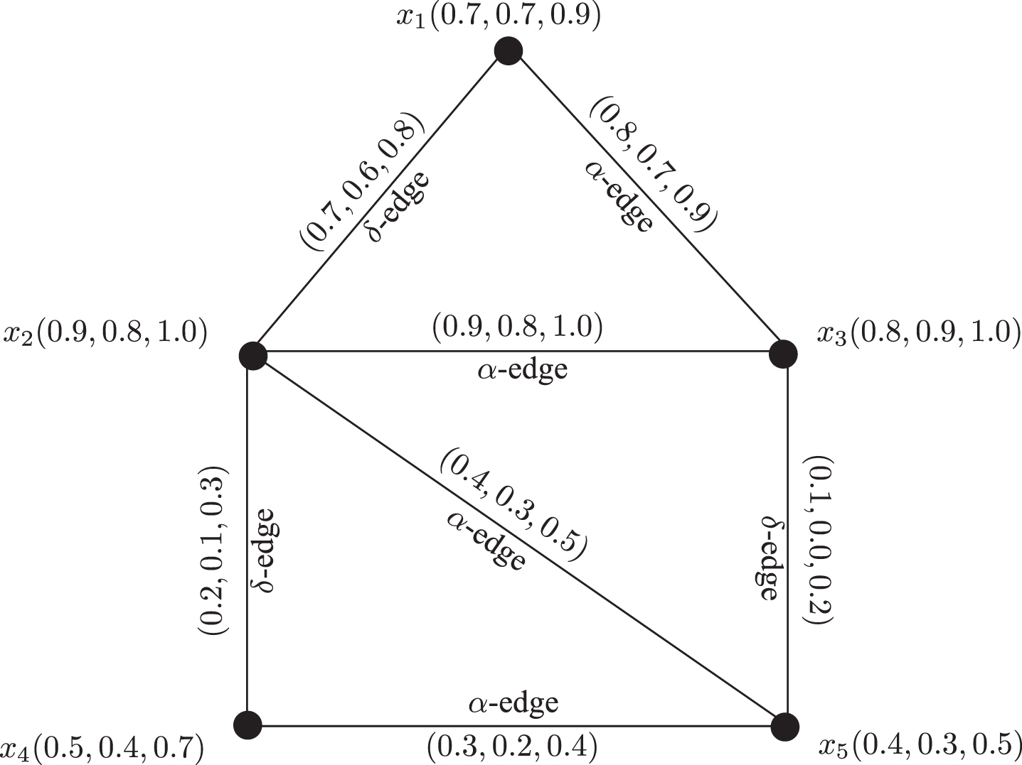
In crisp graph theory, each edge in the network is strong. For this reason edge analysis has no importance in crisp graph theory. However, in mPF graph theory, mPF edges in the mPF graphs are defined as strong mPF edges and non-strong mPF edges [17]. Therefore, mPF edge analysis in mPF graph theory has a significant role and it is very important to determine the nature of an mPF edge in an mPF graph. There is no such analysis on mPF edges in mPF graph theory in the literature. Depending on strength of connectedness between pairs of adjacent vertices of an mPF graph G, we characterize mPF edges according to the following definitions:
Through out this study, we assume that G has no mixed mPF edges.
3PF vertex set
3PF vertex set
3PF edge set

3PF graph.
In network theory, x i -x k separating set X′ of vertices is a collection of vertices in G★ = (X, E) whose removal disconnects G★ into different components G★ \ {x k } and G★ \ {x i } with vertices x i and x k not belong to the same components of G★ \ X′. Similarly, x i -x k separating set E′ of edges is defined. See also [19, 20]. Since, the reduction in strength is more significant and frequent in networks, therefore we define x i -x k strength reducing set of vertices (SRSVs) and x i -x k strength reducing set of edges (SRSEs) in an mPF graph G = (Ψ, Φ) as follows:
In either case vertex x is an mPF cut-vertex of G. □
3PF vertex set
3PF vertex set
4PF edge set
3PF graph.
In either case edge xy is an mPF bridge of G. □
3PF vertex set
4PF edge set

3PF graph.
3PF vertex set
3PF edge set
3PF graph.
{x2, x4, x7}, {x2, x4, x8}, {x2, x4, x9},
{x2, x5, x7}, {x2, x5, x8}, {x2, x5, x9},
{x2, x4, x7, x8}, {x2, x4, x7, x9}, {x2, x4, x8, x9}, {x2, x5, x7, x8},
{x2, x5, x7, x9}, {x2, x5, x8, x9}, {x2, x4, x5, x7}, {x2, x4, x5, x8}, {x2, x4, x5, x9},
{x2, x4, x5, x7, x8}, {x2, x4, x5, x7, x9}, {x2, x4, x5, x8, x9},
{x2, x4, x5, x7, x8, x9}.
3PF vertex set
4PF edge set

3PF graph.
It is interesting to note that in this example minimum x1-x3 SRSVs contains at least three vertices. For instance,
We now present an mPF graph version of one of the famous results in graph theory due to the Karl Menger. For fuzzy version of Menger’s theorem, the readers may read reference [20].
Now, suppose that
Let
Let
We assume on contrary that there exists a minimum x i -x k SRSVs (say U = {u1, u2, …, ut-1}) in G \ {xy} with t-1 vertices. Then U ∪ {x} is a minimum x i -x k SRSVs in G. Also, note that each vertex in the set U ∪ {x}, i.e., u1, u2, …, ut-1 and x is α-strong neighbor of vertex x i . As U ∪ {y} is also a minimum x i -x k SRSVs in G. It follows that vertex y is an α-strong neighbor of vertex x i . This contradicts to the fact that xy is β-edge. (x i x, x i y and xy form a triangle with xy as weakest mPF edge. The unique weakest mPF edge of an mPF cycle is a δ-edge). Hence, t is the minimum number of vertices in an x i -x k SRSVs in G \ {x}. As S S (G \ {x}) < S S (G). By induction, it follows that G \ {xy} has t internally disjoint strongest [x i , x k ]-mPF paths and hence in G.
Let V = {v1, v2, …, v
t
} be the minimum x
i
-x
k
SRSVs having t vertices with the property mentioned in case III. Consider each strongest mPF path from vertex x
i
to vertex x
k
(see in Fig. 8(a)). As V is a minimum x
i
-x
k
SRSVs this implies that vertices v1, v2, …, v
t
must belong to at least one such [x
i
, x
k
]-mPF path. Let G
x
i
be the mPF subgraph of G containing all [x
i
-v
i
]-mPF subpath of each strongest [x
i
, x
k
]-mPF path in which v
i
∈ V is the only vertex of the mPF path belonging to V. Note that if P
j
∘ CONN
G
(x
i
, x
k
) = f
j
then P
j
∘ Φ (xy) ≥ f
j
(where for each 1 ≤ j ≤ m, f
j
be any real number in [0, 1]) for every edge xy in these mPF paths. Let

Construction of mPF subgraphs
Assume that for each 1 ≤ j ≤ m, P
j
∘ Ψ (w) =1 and P
j
∘ Φ (v
i
, w) = P
j
∘ Ψ (v
i
) for all i = 1, 2, …, t. Similarly, mPF subgraphs G
x
k
and
3PF vertex set
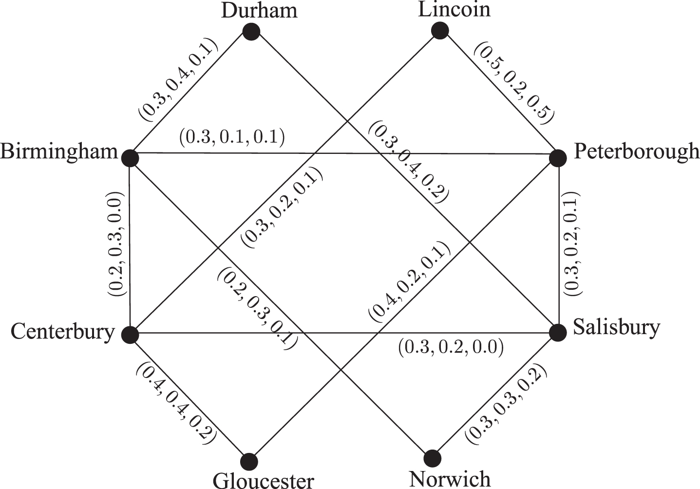
The membership value of each vertex is measured according to three characteristics: {population, city condition, expenses}. The membership value of each edge is measured according to three characteristics: {traffic jam on road, road condition, travel cost}. The membership values of roads are calculated according to the condition: P j ∘ Φ (xy) ≤ inf {P j ∘ Ψ (x) , P j ∘ Ψ (y)} for each 1 ≤ j ≤ m. The correspondent 3PF graph G = (Ψ, Φ) is shown in Fig. 9. Since, Lincoin is the disaster area, it needs help from non-disaster cities through efficient roots. For this purpose, we will find out the strongest mPF paths from non-affected cities to Lincoin. Consider two cities Centerbury and Lincoin (not strong neighbors of each other). The mPF paths from Centerbury to Lincoin with their corresponding strengths are:
P1: Centerbury - Lincoin, S (P1) = (0.3, 0.2, 0.1)
P2: Centerbury - Birmingham - Peterborough - Lincoin, S (P2) = (0.2, 0.1, 0.0)
P3: Centerbury - Salisbury - Peterborough - Lincoin, S (P3) = (0.3, 0.2, 0.0)
P4: Centerbury - Gloucester - Peterborough - Lincoin, S (P4) = (0.4, 0.2, 0.1)
The minimum {Centerbury}-{Lincoin} SRSVs in this network consists of only one vertex, i.e., X′ = {Peterborough}. According to Theorem 4.5 there is only one internally disjoint strongest mPF path from Centerbury to Lincoin, i.e., P4 (CONN G (Centerbury, Lincoin) = (0.4, 0.2, 0.1) = S (P4)). Therefore, Centerbury has to send essentials to Lincoin through strongest mPF path P4. Similarly, we can find out strongest mPF paths from other non-affected cities to Lincoin.
3PF graph
We now discuss the edge version of Menger’s Theorem for mPF graphs.
Now, suppose that
Let
Let
We assume on contrary that there exists a minimum x i -x k SRSEs (say H = {e1, e2, …, et-1}) in G \ {xy} with t-1 edges. Then H ∪ {xy} is a minimum x i -x k SRSEs in G. Also, note that each edge in the set H ∪ {xy}, i.e., e1, e2, …, et-1 and xy is incident with vertex x i such that x is α-strong neighbor of vertex x i . As H ∪ {xz} is also a minimum x i -x k SRSEs in G. It follows that vertex yz is incident with vertex x i such that z is an α-strong neighbor of vertex x i . This contradicts to the fact that xz is β-edge. Hence, t is the minimum number of edges in an x i -x k SRSEs in G \ {xy}. As S S (G \ {xy}) < S S (G). By induction, it follows that G \ {xy} has t internally disjoint strongest [x i , x k ]-mPF paths and hence in G.
Let F = {f0 = v0v1, f1 = v1v2, …, ft-1 = vt-1v
t
} be the minimum x
i
-x
k
SRSEs having t edges with the property mentioned in case III. Consider each strongest mPF path from vertex x
i
to vertex x
k
(see in Fig. 8(a)). As F is a minimum x
i
-x
k
SRSEs this implies that edges f0, f1, …, ft-1 must belong to at least one such [x
i
, x
k
]-mPF path. Let G
x
i
be the mPF subgraph of G containing all [x
i
-v
i
]-mPF subpath of each strongest [x
i
, x
k
]-mPF path in which f
i
∈ F is the only edge of the mPF path belonging to F with one of its end vertex v
i
. Note that if P
j
∘ CONN
G
(x
i
, x
k
) = q
j
then P
j
∘ Φ (xy) ≥ q
j
(where for each 1 ≤ j ≤ m, q
j
be any real number in [0, 1]) for every edge xy in these mPF paths. Let
Assume that for each 1 ≤ j ≤ m, P
j
∘ Ψ (z) =1 and P
j
∘ Φ (v
i
, z) = P
j
∘ Ψ (v
i
) for all i = 1, 2, …, t. Similarly, mPF subgraphs G
x
k
and
Theorem 4.5 only able to provide maximum number of internally disjoint strongest [x i , x k ]-mPF paths in G if x i and x k both are not strong mPF neighbors of each other, i.e., x i x k is not strong mPF edge. If x i and x k both are strong mPF neighbors of each other then Theorem 4.5 can not be applied. However, Theorem 4.6 provides the maximum number of internally disjoint strongest [x i , x k ]-mPF paths in G no matter x i and x k both are strong mPF neighbors of each other or not. For illustration, consider two cities Peterborough and Lincoin in Example 4.7. Peterborough and Lincoin are strong mPF neighbors of each other. The minimum Peterborough-Lincoin SRSVs consists of no vertex. So, we are not able to apply Theorem 4.5 here to find out maximum number of internally disjoint strongest [Peterborough, Lincoin]-mPF paths. However, minimum Peterborough-Lincoin SRSEs consists of one edge, i.e., edge between Peterborough and Lincoin. Therefore, we can apply Theorem 4.6 here to find out maximum number of internally disjoint strongest [Peterborough, Lincoin]-mPF paths.
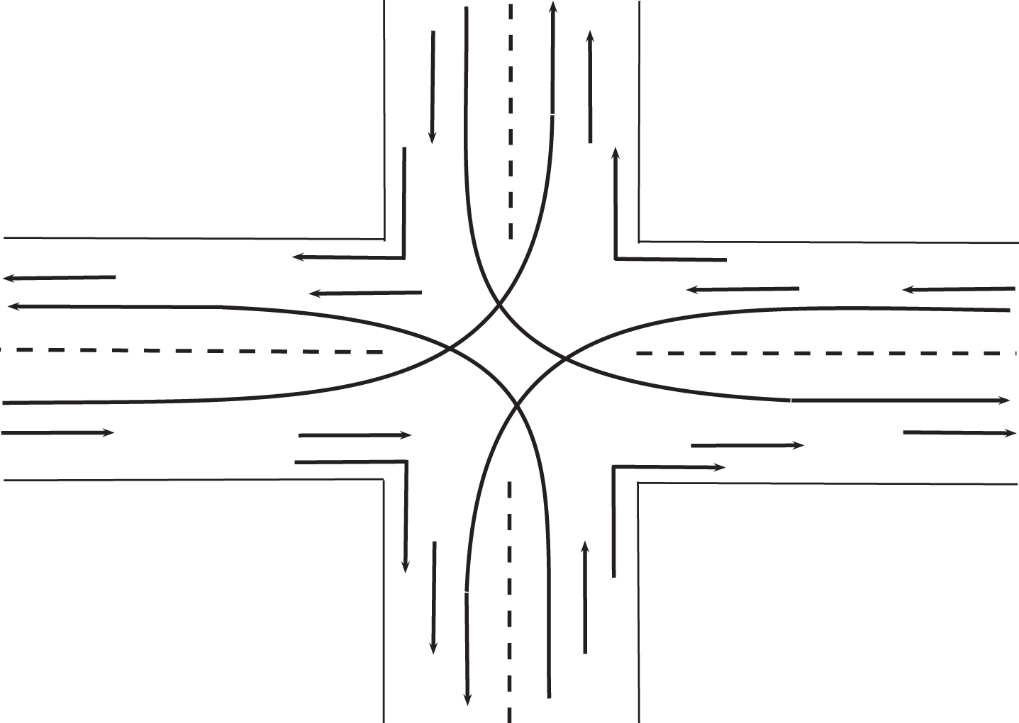
A fuzzy graph is actually a convenient way of representing information involving relations between vague or uncertain objects. The vague objects are taken as fuzzy vertices while relationships between them by fuzzy edges. Fuzzy graphs involve membership values of vertices and edges with respect to single attribute only. However, we have to deal with multi-objects, multi-agents or multi-polar information in many real-world vague problems. To illustrate such type of problems, mPF graphs provide more precision and accuracy as compared to fuzzy graphs. In this paper, we highlight the types of traffic-accidental zones in a road network with the help of strength of connectedness between traffic intersections in the road network. Nowadays, road accidents have become very common. Data analysis shows that road accidents depend upon multi-factors like road condition, vehicles on the road, careless driving, over speeding, reckless driving, construction sites, etc. Road accidents are more likely to occur at traffic intersections. We need to develop a flow pattern so that vehicles can pass through the intersections without interfering with other traffic flows. Since, road accidents depend upon multi-factors. Therefore, we can represent the road network as an mPF graph network. For this purpose, we consider a road network as shown in Fig. 11.

Construction of mPF subgraphs
Road network.
In Fig. 11, each direction indicates the traffic flow from one side of the road to another side of the road. However, the road condition, vehicles on road, reckless driving in all directions are not always the same. All these factors are fuzzy in nature. Due to this reason, we consider it as an mPF set where membership value depends on {road condition, vehicles on road, reckless driving}. It can easily be observed in Fig 11 that each right directed traffic flow does not intersect with the other traffic flows. So, we can eliminate these directions from our further discussion. The remaining directions are shown in Fig. 12.
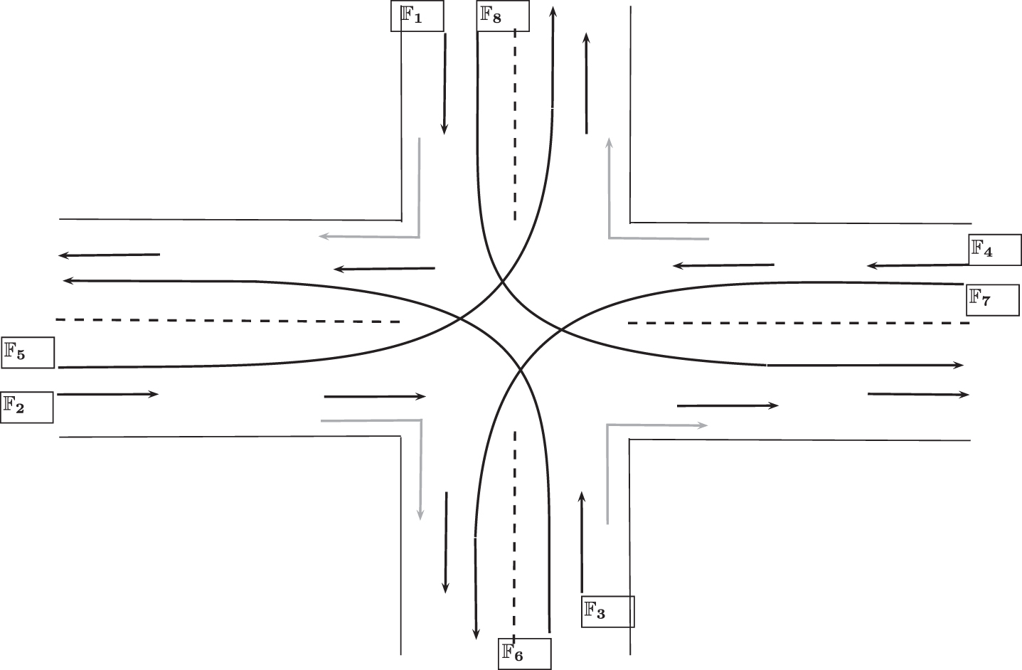
Labeled road network
In Fig. 12, let us label all directions of traffic flow on the road. Let
3PF vertex set
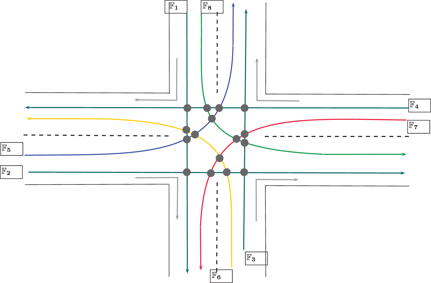
Crossings between different traffic flows
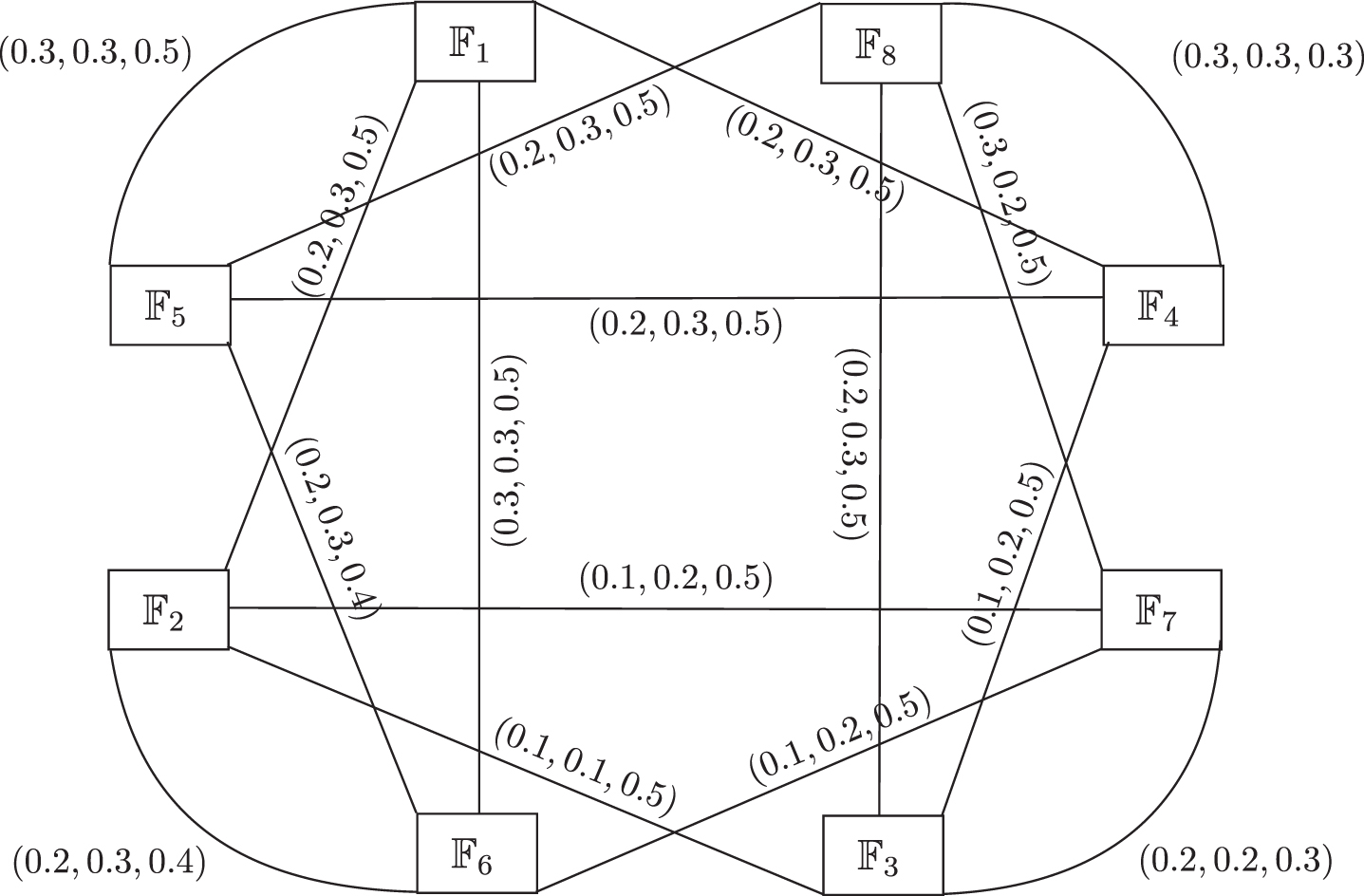
mPF graph network
We now present the procedure of our application in the following algorithm.
The flowchart of above algorithm is given in Fig. 15.
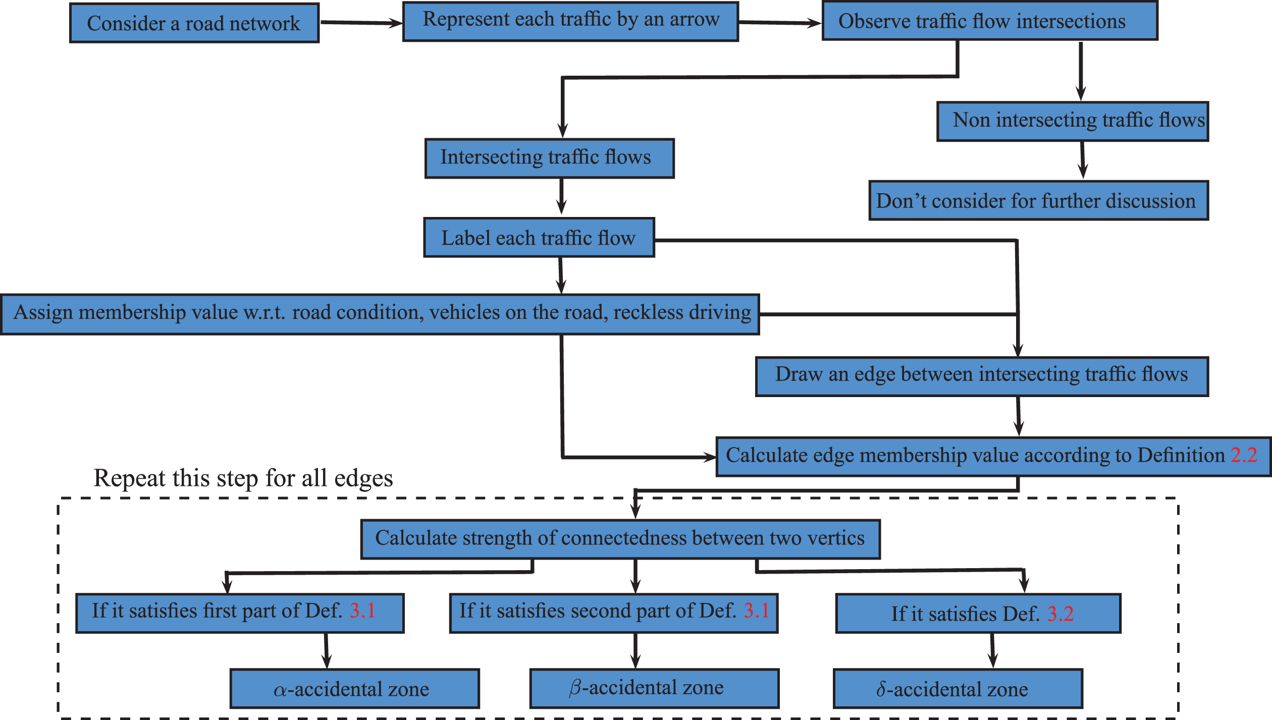
Flowchart of road network problem
The strength of connectedness between any pair of vertices in a crisp graph is either 0 or 1 as there is an edge between two vertices or not. For this reason, edge analysis in case of crisp graphs provides no information. Fuzzy graph is an extension of a crisp graph. In fuzzy graphs, all vertices and edges are uncertain in nature and their membership value can be any real number in [0, 1]. Due to the existence of membership value, edge analysis is important to understand the nature of each edge and basic structure of fuzzy graph. In fuzzy graph, membership value corresponds to a single uncertain statement. However, many real life problems are multi-polar uncertain in nature. Fuzzy graphs are unable to efficiently handle vague multi-polarity of any problem. Let us take an example of 4 countries, including China, America, Pakistan and India. All these countries are different according to their population, army position, resources, etc. Similarly, the relationships among these countries may be different according to friendship, enemy relationship, occupying other country relationships, etc. All these terms are vague in nature. We want to discuss the nature of each relationship between two countries. Although, edge analysis in fuzzy graph provides such information but fuzzy graph does not efficiently handle the existing problem. To discuss each relationship, we have to make a separate fuzzy graph (shown in the following Fig. 16).
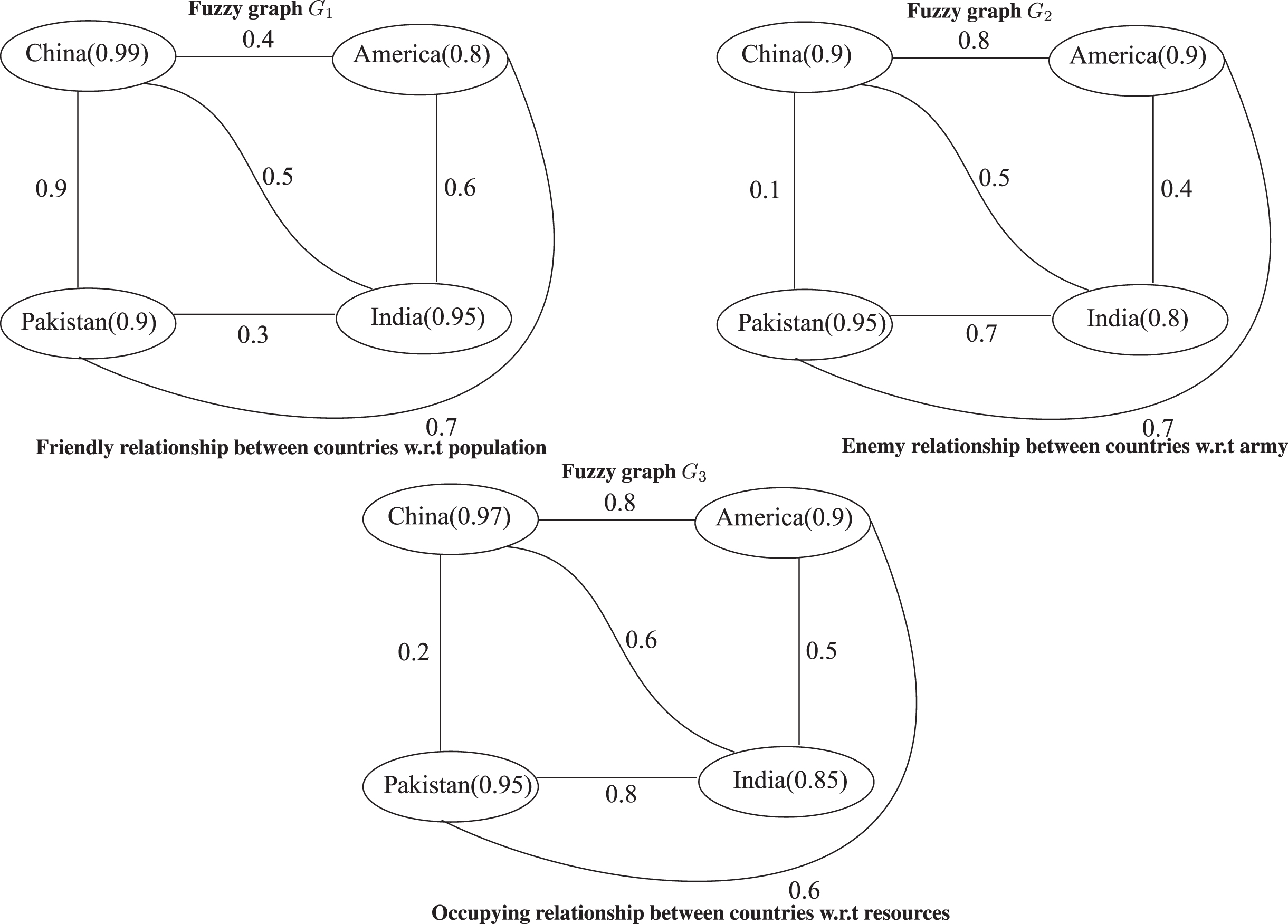
Fuzzy graphs representing relationships among countries
Consider two countries, Pakistan and America. All possible paths from Pakistan to America with their strengths and strength of connectedness between Pakistan and America are given below:
P1: Pakistan - America S (P1) =0.7
P2: Pakistan - India - America S (P1) =0.3
P3: Pakistan - China - America S (P1) =0.4
P4: Pakistan - India - China - America S (P1) =0.3
P5: Pakistan - China - India - America S (P1) =0.5
CONN G 1 (Pakistan, America) =0.7
CONNG1\{Pakistan,America} (Pakistan, America) =0.5
P1: Pakistan - America S (P1) =0.7
P2: Pakistan - India - America S (P1) =0.4
P3: Pakistan - China - America S (P1) =0.1
P4: Pakistan - India - China - America S (P1) =0.4
P5: Pakistan - China - India - America S (P1) =0.1
CONN G 2 (Pakistan, America) =0.7
CONNG2\{Pakistan,America} (Pakistan, America) =0.4
P1: Pakistan - America S (P1) =0.6
P2: Pakistan - India - America S (P1) =0.5
P3: Pakistan - China - America S (P1) =0.2
P4: Pakistan - India - China - America S (P1) =0.6
P5: Pakistan - China - India - America S (P1) =0.2
CONN G 3 (Pakistan, America) =0.6
CONNG3\{Pakistan,America} (Pakistan, America) =0.6
It can be observed that the edge between Pakistan and America is a strong edge in each fuzzy graph G1, G2, G3. Similarly, the edges between other countries can be analyzed. It is difficult and time consuming to deal with each relationship separately and to discuss the nature of each edge. An mPF graph is an extended approach of a fuzzy graph. In an mPF graph, all vertices and edges are multi-polar uncertain in nature and their membership values have multi-components according to the multi-polar uncertain statements. In which each component of membership value can be any real number in [0, 1]. All these components are independent from each other. An mPF graph is an efficient approach to discuss several relationships among countries at a time. For example, consider China, America, Pakistan and India as 3PF vertices. The membership value of each country is measured according to the population, army, resources of that country. The description of each country can be written in the form of a set as: {Population, Army, Resources}. The relationship between countries is represented by 3PF edges. The membership value of each edge is measured according to the friendship, enemy relationship, occupying relationship between countries. The description of each edge can be written in the form of a set as: {Friendship, Enemy relationship, Occupying relationship}. The correspondent 3PF graph is shown in Fig. 17.
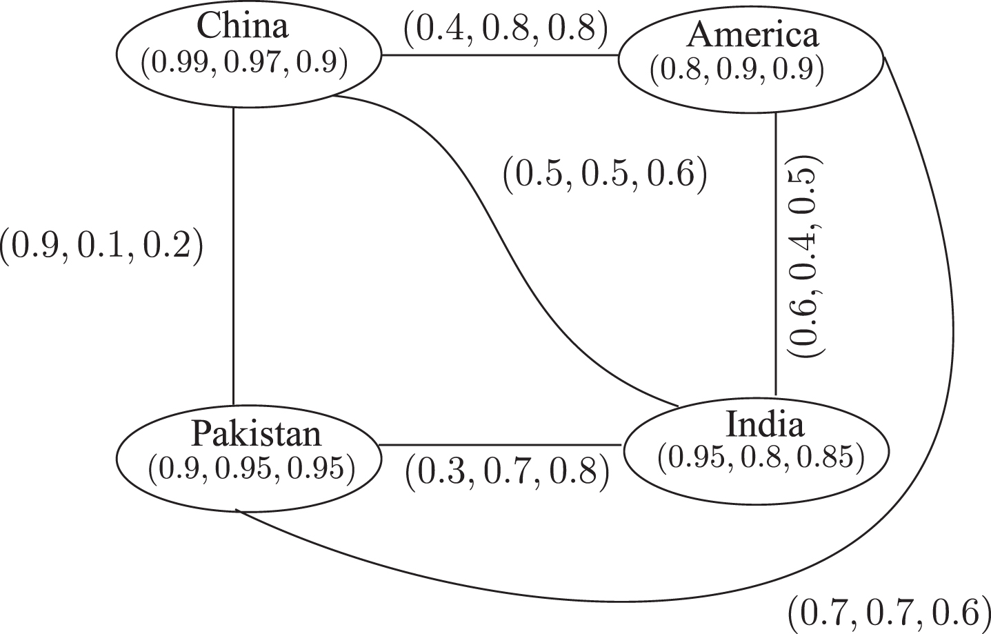
3PF graph representing relationships among countries
We now consider, Pakistan and America. All possible paths from Pakistan to America with their strengths and strength of connectedness between Pakistan and America are given below:
P1: Pakistan - America S (P1) = (0.7, 0.7, 0.6)
P2: Pakistan - India - America S (P1) = (0.3, 0.4, 0.5)
P3: Pakistan - China - America S (P1) = (0.4, 0.1, 0.2)
P4: Pakistan - India - China - America S (P1) = (0.3, 0.4, 0.6)
P5: Pakistan - China - India - America S (P1) = (0.5, 0.1, 0.2)
CONN G (Pakistan, America) = (0.7, 0.7, 0.6)
CONNG\{Pakistan,America} (Pakistan, America) = (0.5, 0.4, 0.6)
It can observe that 3PF edge between Pakistan and America is strong 3PF edge. Similarly, the edges between other countries can be analyzed. It takes less time to discuss nature of each edge in an mPF graph. This proves the applicability and efficiency of our research work.
An mPF graph plays a significant role in modeling of real-world problems that involve multi-attribute, multi-polar information and uncertainty. The mPF graphs provide accurate and flexible results when we have to deal with more than one agreements or suggestions. There are still many fuzzy graph theoretic results which have not been yet studied in case of mPF graph theory, e.g., edge analysis, vertex and edge connectivity parameters etc. In this research study, we have defined strong mPF edges and weak mPF edges with the help of strength of connectedness between pairs of vertices. We have presented Menger’s theorem for mPF graphs and illustrated it by an example. We have discussed an application to determine traffic-accidental zones in a road network with the help of types of mPF edges. Moreover, we have designed an algorithm (flowchart) to elaborate the procedure of our application. In future, we want to extend our research work to vertex connectivity and edge connectivity parameters for mPF graphs.
Conflict of interest
The authors declare no conflict of interest.
Footnotes
Acknowledgement
This project is funded by NRPU project no. 9073, HEC Islamabad.