
Abstract
Due to the promising performance on energy-saving, the building integrated photovoltaic system (BIPV) has found an increasingly wide utilization in modern cities. For a large-scale PV array installed on the facades of a super high-rise building, the environmental conditions (e.g., the irradiance, temperature, sunlight angle etc.) are always complex and dynamic. As a result, the PV configuration and maximum power point tracking (MPPT) methodology are of great importance for both the operational safety and efficiency. In this study, some famous PV configurations are comprehensively tested under complex shading conditions in BIPV application, and a robust configuration for large-scale BIPV system based on the total-cross-tied (TCT) circuit connection is developed. Then, by analyzing and extracting the feature variables of environment parameters, a novel fast MPPT methodology based on extreme learning machine (ELM) is proposed. Finally, the proposed configuration and its MPPT methodology are verified by simulation experiments. Experimental results show that the proposed configuration performs efficient on most of the complex shading conditions, and the ELM-based intelligent MPPT methodology can also obtain promising performance on response speed and tracking accuracy.
Keywords
Introduction
Due to the world-wide environment problem caused by fossil fuel burning, different kinds of renewable energy systems are widely adopted to generate electricity power by exploring clean energy [1–3]. As one of the most popular renewable energy systems, the photovoltaic (PV) power generation system is widely used in real engineering applications, for example, the grid-connected PV system [4], the green ship with PV system installed [5–7], the hybrid green energy system and so on [8].
The building integrated photovoltaic system (BIPV), which means that thousands of PV modules are installed on the facades of a building to collect the solar energy, has found an increasingly wide utilization in modern cities [9, 10]. As buildings account for almost 32% of the world’s total energy consumption, it is of great value to develop the green buildings and even near net-zero energy buildings [11]. By installing large-scale PV array on the building’s surface, the BIPV system makes use of the building envelope for solar energy collection, providing an efficient way of generating electricity power and reducing building energy consumption.
As the energy harvesting component, the PV array in BIPV system is usually composed of many PV modules in certain connections. For BIPV system installed on a super high-rise building, the shadings of PV array are always complex and dynamic. This may significantly reduce the entire power output, and may also cause permanent thermal damage of PV modules [12]. To be specific, the detailed reason for integrating the maximum power point tracking (MPPT) control in BIPV system can be illustrated as the following two aspects: on one hand, the output power of BIPV array will be maximized in real-time by the integrated MPPT system. For a certain connected PV array without MPPT, the partial shading will cause significant power loss to not only the shaded PV modules but also the un-shaded modules nearby. Obviously, this additional power loss greatly reduces the system efficiency, especially for the BIPV system which always operates in complex and dynamic shading conditions; on the other hand, the effective PV configuration and MPPT control method can also protect PV module from the “hot-spot” effect caused by deep partial shading. As discussed above, the optimal configuration of large-scale BIPV system and its MPPT control methodology are of great importance for system operational safety and efficiency [13].
In the past decades, as the PV systems are often integrated into small buildings, the adopted MPPT methods are always the basic constant voltage control (CV), the perturb and observe (P&O), or the incremental conductance (InC). However, due to the development of green building and intelligent building in recent years, the large-scale PV system begins to be integrated into the super high-rise buildings in modern city [14]. Obviously, the traditional MPPT methods like CV, P&O, and InC are not efficient enough for these large-scale BIPV system due to the huge PV module quantity and unpredictable occupants’ behaviours. As a result, the lack of efficient MPPT system is actually a major problem for the large-scale BIPV system, and obviously it is worthy to be discussed in detail. This study compares and analyses different PV configurations under typical shading conditions in BIPV application, and an optimal configuration based on total-cross-tied (TCT) circuit connection is developed. In addition, a novel fast MPPT methodology based on extreme learning machine (ELM) is also proposed for improving the MPPT performance, especially under complex and dynamic shading conditions of large-scale BIPV system.
The rest of this study is organized as follows: Section 2 presents an overview of the related works, including the BIPV system, configuration of PV array and some state-of-the-art MPPT methodologies. Section 3 compares and analyses some popular PV configurations in BIPV application. Section 4 presents the TCT-based configuration of large-scale BIPV system. In Section 5, the ELM-based fast MPPT model is established by extracting the environmental feature variables. The experimental results and analysis are conducted in Section 6. Finally, this study is concluded in Section 7.
As discussed above, the main contributions of this study can be summarized as the following points: Comparison for typical PV array configurations in building application Novel configuration for large-scale building integrated PV system Feature extraction for environmental parameters under complex shading condition Structures and comparison of data-driven maximum power point tracking model Fast maximum power point tracking methodology based on extreme learning machine
Related works
Building integrated photovoltaic system
In BIPV system, the PV modules are adopted as construction material in the design and construction processes, for example, PV window overhangs and BIPV shingles on the roof. Obviously, the energy-saving performance of a building can be enhanced by the use of BIPV system. Due to the promising energy performance, the installation of BIPV system on modern buildings is a hot topic and attracts attentions of world-wide scholars [15].
For example, Lu et al. introduced the PV system into an isolated building [16], and the effect of dust pollution on the performance of BIPV system is also analysed in their study. In order to verify the electrical properties of BIPV system, Sprenger et al. evaluated the performance on electricity power generation of a complex BIPV system, which is installed in the main building of Fraunhofer Institute for Solar Energy Systems [17]. Ravyts et al. proposed a methodology for investigating the influence of feeder voltage level and solar cell technology on the efficiency of facade BIPV system [18]. Salameh et al. evaluated the performance of BIPV system in commercial application, especially when the cooling load is high. According to the result of their case study, the use of BIPV system can save the power consumption of air conditioning system by 27.69%, and reduce the annual power cost by 2084 $ [19].
Configuration of photovoltaic system
As the output voltage of a single PV cell is very small, a PV module is usually composed of several PV cells in series connection. Similarly, a PV array is also composed of many modules in certain connection. The PV configuration, which means the connection of all the PV modules to form a certain scale array, is very important to the overall performance. Especially under partial shading conditions, an efficient PV configuration may significantly improve the entire output power [20].
The most widely used PV configuration contains the basic series configuration (S), the classical series-parallel configuration (SP), total-cross-tied configuration (TCT), honey-comp (HC) configuration, bridge-linked (BL) configuration and so on [21]. For further improving the performance under partial shading conditions, some new PV configurations are widely developed. For example, Bosco et al. proposed a novel cross diagonal view configuration for improving the output power under partial shading condition [22]. Rani et al. developed a methodology to arrange the PV modules in a TCT connection using the Su Do Ku puzzle pattern, in order to distribute the shading effect over the entire array, and improve the overall performance under partial shading condition [23]. In our previous work, the configuration of large-scale PV system is discussed [24]. Based on the proposed configuration, MPPT control at the level of PV module, and at the level of minimum control unit are achieved. In addition, the configurations of large-scale PV array in some special engineering applications (e.g., the large green ships, the BIPV system) are also developed in our previous works [25, 26].
Maximum power point tracking
As the PV output is easily affected by environment conditions, e.g., the irradiance, temperature, and shading, the MPPT is very necessary for a PV system to reduce this effect and maintain maximum output. The existing MPPT methods can be divided into two categories, that is, the online MPPT and offline MPPT. For the first online MPPT, the most widely used method is the P&O, InC and their variants. For example, Pilakkat et al. proposed an improved P&O by introducing the artificial bee colony algorithm. According to their simulation results, the proposed P&O-variant gave more than 99.5% efficiency under partial shading conditions [27]. Alik et al. developed a modified P&O by adding the so-called checking mechanism. Experimental results showed that their proposed P&O method can obtain even 100% tracking efficiency under partial shading conditions [28].
For the offline MPPT, Huang et al. developed a data-driven approach called the spline model guided MPPT method, in order to benefit the PV power generation facing variable partial shading conditions [29]. Mao et al. proposed a maximum power exploitation method for grid-connected PV system by employing the salp swarm algorithm, in order to overcome the influence caused by the fast-varying environment conditions [30]. In our previous work, we proposed a data-driven MPPT method, in which the time-window mechanism was employed to overcome the existed problems in maritime application [31]. In addition, the offline MPPT methods based on machine learning model, evolutionary algorithm and some other intelligent approaches are interesting topics and attract worldwide attentions [32–34].
Comparison of PV configurations for BIPV application
The shadings of BIPV system
The BIPV system has been identified as one of viable technologies to improve the building energy performance. For a BIPV system installed on a super high-rise building, it involves combing PV power generation technologies with typical building fabrics such as the roof and facades. In particular, the roof and facades are completely covered by a special PV module namely the BIPV window, which has been verified to have excellent optical, thermal and power-generating properties [35]. For the BIPV window, the solar cells incorporated in a typical window can generate electricity power, which therefore reduces the off-side power demand, and yet allow daylight which enhances occupants’ visual comfort. The application of BIPV system are shown as Fig.1.
As shown in Fig. 1, the PV array of a BIPV system always contains a large number of PV modules installed on the roof or facades. Due to the special working environment, the PV array always suffers from the partial shading conditions (PSC), or even complex and dynamic shading conditions (CSC/DSC). The reasons are analysed as follows:

The application of BIPV system.
On one hand, the BIPV system may be shaded by the clouds, dusts or litters, and the shadows of surrounding buildings. On the other hand, each of the BIPV windows may be open or closed at each time, and the angles of them are even random. That is because the BIPV windows are not only the power generation units, but also the traditional windows for the building. As a result, each of the BIPV windows may be opened to a certain degree by the occupants, and this may affect the incidence angle of sunlight, and may also cause partial shadings for the lower windows. The complex shading of BIPV system is illustrated in Fig. 2.
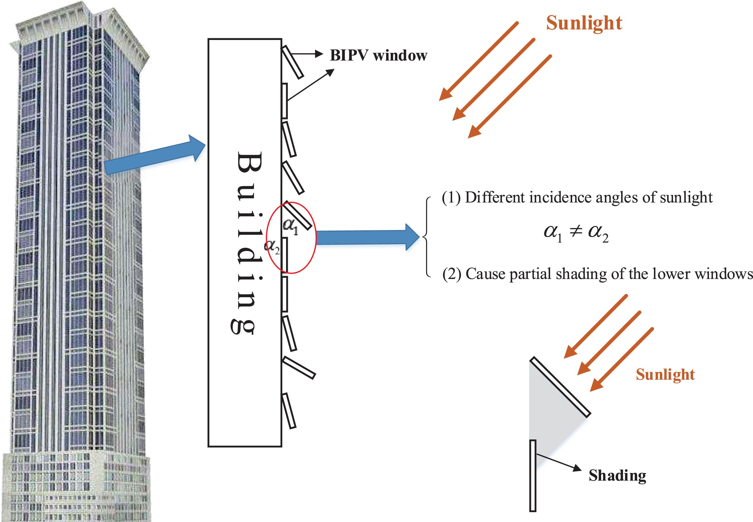
Complex shadings of BIPV system.
Note that in Fig. 2, the status of BIPV window (means closed/open, and the opening degree) may be dynamically changed due to the huge window quantity and the unpredictable occupants’ behaviours. As a result, the complex shadings (i.e., CSC) in Fig. 2 are always combined with the dynamic characteristics (i.e., DSC), which makes the real-time MPPT control of BIPV system more difficult.
In order to optimally connect all the BIPV windows to overcome the aforementioned CSC and DSC environments, some well-known PV configurations are compared under some typical shading conditions of BIPV system. The compared PV configurations include the series configuration (S), series-parallel configuration (SP), total-cross-tied configuration (TCT), bridge-linked configuration (BL), and the honey-comb configuration (HC) [20-21], which are illustrated in Fig. 3.
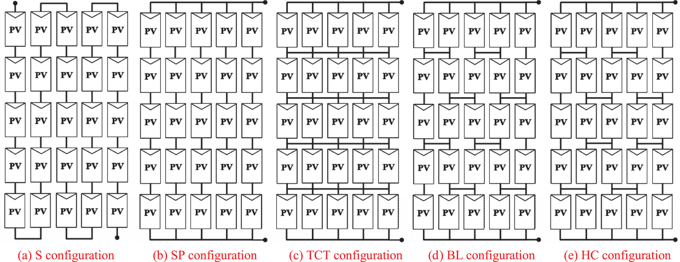
Schematics the S, SP, TCT, BL, and HC configurations.
As discussed above, the shadings of BIPV system are much more complex than the other applications due to the unpredictable behaviours of occupants. In this section, the aforementioned 5 classic PV configurations are compared under CSC conditions. The employed shading conditions of BIPV system are shown in Fig. 4. Note that in Case 1, the irradiance is almost uniform except a few individual BIPV windows. In Case 2, the shadings become complex and the irradiance is non-uniform. In Case 3 to 5, the PV array is totally under CSC, especially for Case 4, the irradiance of each adjacent BIPV window is different, and for Case 5, the irradiance of each BIPV window is randomly generated between 50 W/m2 to 1000 W/m2. As discussed above, the shading complexity increases from Case 1 to 5.

Shading conditions of BIPV system.
Parameters of the PV module adopted in comparison experiments are as follows: the short-circuit current under reference environment condition (I Scref ) is 8.24 A; the open circuit voltage under reference condition (V Ocref ) is 40.35 V; the current of maximum power point (MPP) under reference condition (I mref ) is 7.36 A; the voltage of MPP under reference condition (V mref ) is 31.25 V. The simulation software is MATALB/SIMULINK R2019b. The Power-Voltage (P - V) characteristics of each configuration for different cases are plotted in Fig. 5.
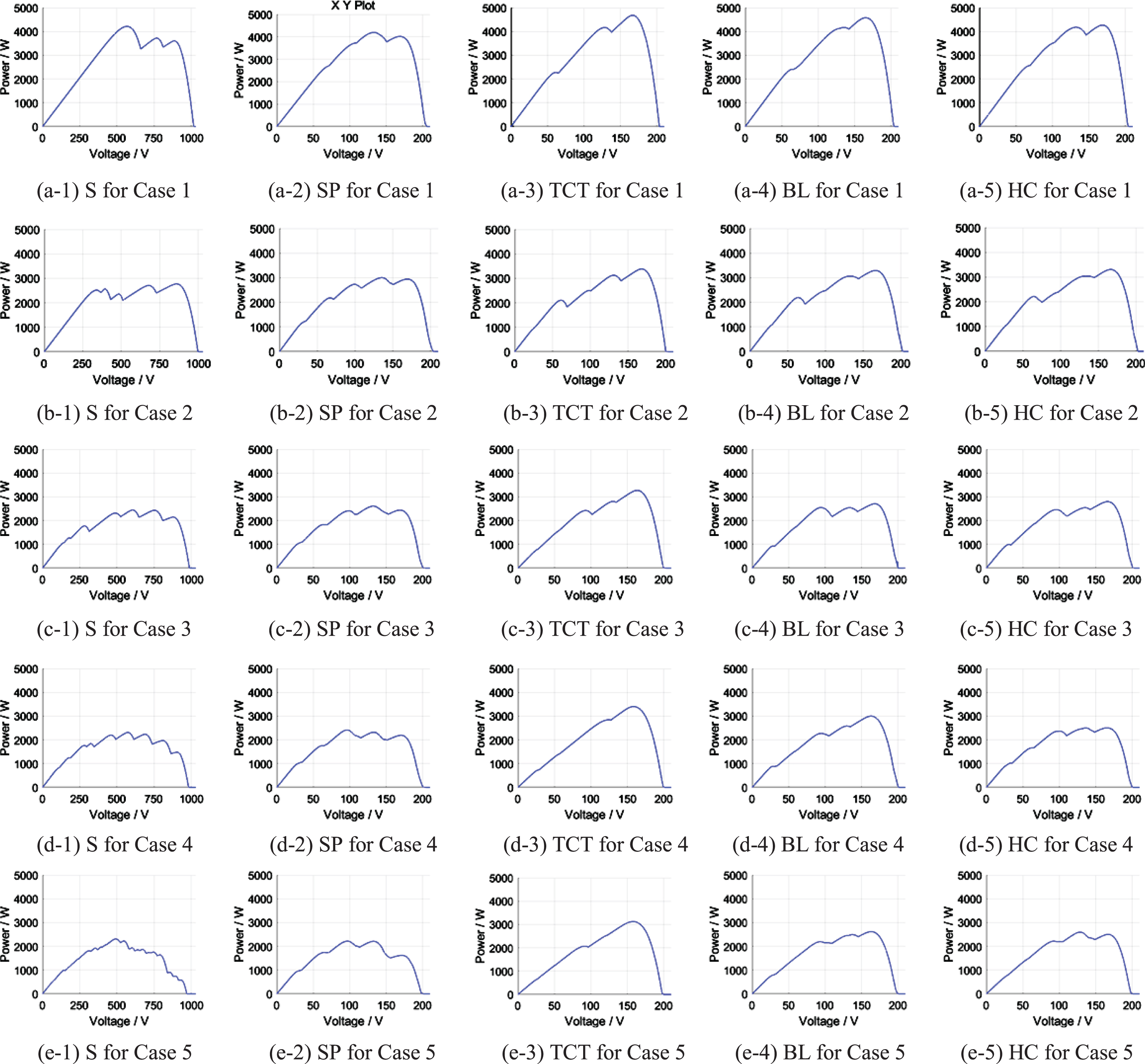
P-V characteristics for each configuration.
As shown in Fig. 5, the P-V characteristics for the above configurations are different under partial shading conditions. Especially when the CSC occurs in Case 3 to 5, a lot of local optimums exist in the P-V curves of S and SP configurations. However, the local optimums for TCT, BL and HC are relatively few. The maximum output power for the above configurations are compared in Table 1, in which the best performance is set in bold.
Maximum output power for each configuration
As shown in the table, TCT outperforms the other configurations for all the cases. However, S performs the worst for Case 2 to 4, and SP performs the worst for Case 1 and Case 5. The outperformance of TCT compared with other configurations is listed in Table 2. Note that in Table 2, ηTCT-X denotes the power improvement percentage between the best performer TCT and the competitor X. For example, ηTCT-SP denotes the power improvement percentage of TCT when compared with SP.
Outperformance of TCT compared with other configurations
As shown in Table 2, when the partial shading condition is not very complex in Case 1 and Case 2, the outperformance of TCT is also not very significant. For example, in Case 2, compared with S and SP, ηTCT-S and ηTCT-SP are 22.08% and 12.73% respectively. In addition, compared with BL and HC, ηTCT-BL and ηTCT-HC are just 2.75% and 2.34%. However, when the shading becomes complex in Case 3, the outperformance of TCT increases to 33.87%, 25.39%, 20.82% and 16.84% compared with S, SP, BL and HC, respectively.
In Case 4 and Case 5, when more complex CSC conditions are imposed on the BIPV windows, the outperformance of TCT becomes very significant. For example, compared with S and SP, ηTCT-S and ηTCT-SP increase to more than 40%. In addition, compared with BL and HC, the outperformance of TCT also increases to different degrees.
As discussed above, it can be concluded that for the complex CSC condition which frequently occurs in BIPV system, the advantage of TCT-based configuration is very significant. Moreover, the advantage of TCT will also increase when the CSC becomes more complex.
In this section, the TCT-based configuration of large-scale BIPV system is developed. To be specific, considering the promising performance of TCT configuration under CSC conditions, the entire BIPV array is divided into several TCT-based sub-arrays. Then, these sub-arrays are installed on each side of the building’s facade for collecting solar energy. Moreover, for a super high-rise building, the facades which can be installed with BIPV windows are always very narrow and long. As a result, the physical-layout of BIPV windows and their circuit-connections are designed to be different. That is to say, each parallel branch in a TCT configuration may correspond to several layers of BIPV window in the building’s physical-layout. The aforementioned TCT-based BIPV configuration, and the relationship between physical-layout and circuit-connection of BIPV windows are illustrated in Fig. 6.
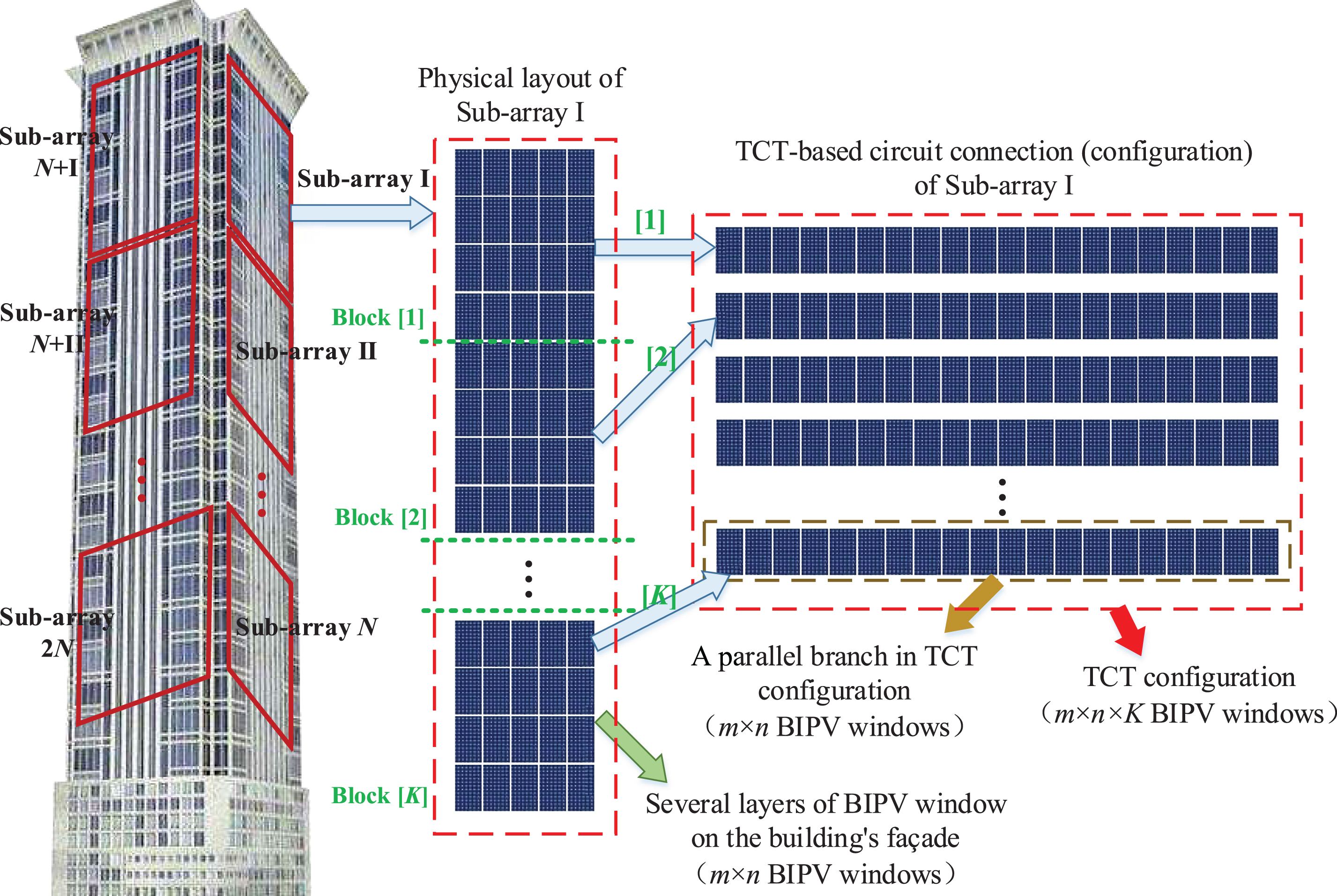
TCT-based BIPV configuration and the relationship between physical layout and circuit connection.
Note that in Fig. 6, the BIPV windows installed on each side of the narrow and long facade are divided into K blocks, and each block consists of m rows and n columns of BIPV windows in physical layout. Then, the BIPV windows within each block are connected as a TCT parallel circuit branch, and the TCT series circuit branches are composed of different blocks. Finally, the irradiance and temperature sensors are equipped within each BIPV blocks. That is to say, the resolution ratios of irradiance and temperature in the proposed configuration are in the level of each BIPV block from the perspective of physical layout, or in the level of each TCT parallel branch from the perspective of circuit connection. Obviously, the scale of each BIPV block (i.e., resolution ratios of the collected irradiance and temperature) can be flexibly designed in certain engineering applications by balancing the hardware cost and MPPT benefit.
As discussed in Section 3, the BIPV system always suffers from the complex and dynamic CSC/ DSC conditions due to the huge window quantity and unpredictable occupants’ behaviours. As a result, the BIPV system requires an efficient MPPT algorithm with high response speed and tracking accuracy, which is significantly difficult than the traditional applications.
In recent years, the data-driven networks, as well as the non-iterative approaches are fast developed and widely applied in many engineering aspects [36–38]. In this section, the extreme learning machine (ELM) is employed to establish the fast MPPT model. ELM was originally proposed for the single-hidden-layer feedforward neural network. Due to the efficient learning efficiency and promising performance on generalization ability, ELM is widely adopted to solve the real engineering problems in recent years [39]. Different from the traditional machine learning model, ELM tends to reach not only the smallest training error but also the smallest norm of output weights. In addition, the hidden layer of ELM network needs not be tuned during training. Schematic of an ELM network is illustrated as Fig. 7.
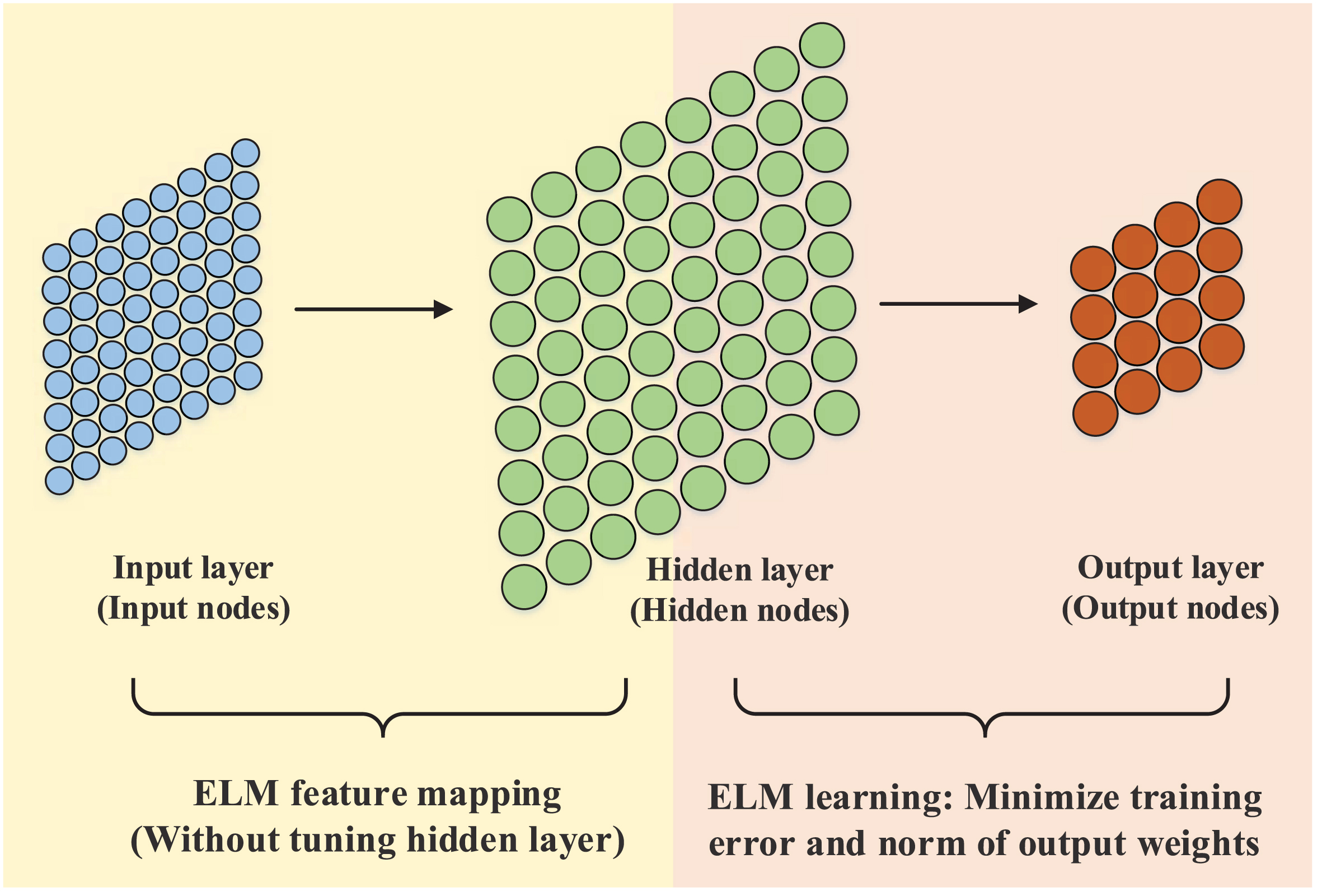
Schematic of ELM network.
As discussed in Section 4, the irradiance and temperature sensors are equipped within each BIPV block. For a BIPV sub-array with K blocks and each block contains m rows and n columns of BIPV windows, i.e., the corresponding circuit connection is a (m · n) × KTCT-based configuration, the environmental variables for each CSC contain K irradiances (S1, S2, ... , S K ) and K temperatures (T1, T2, ... , T K ). The evaluated BIPV sub-array and its environmental variables under CSC are illustrated as Fig. 8.
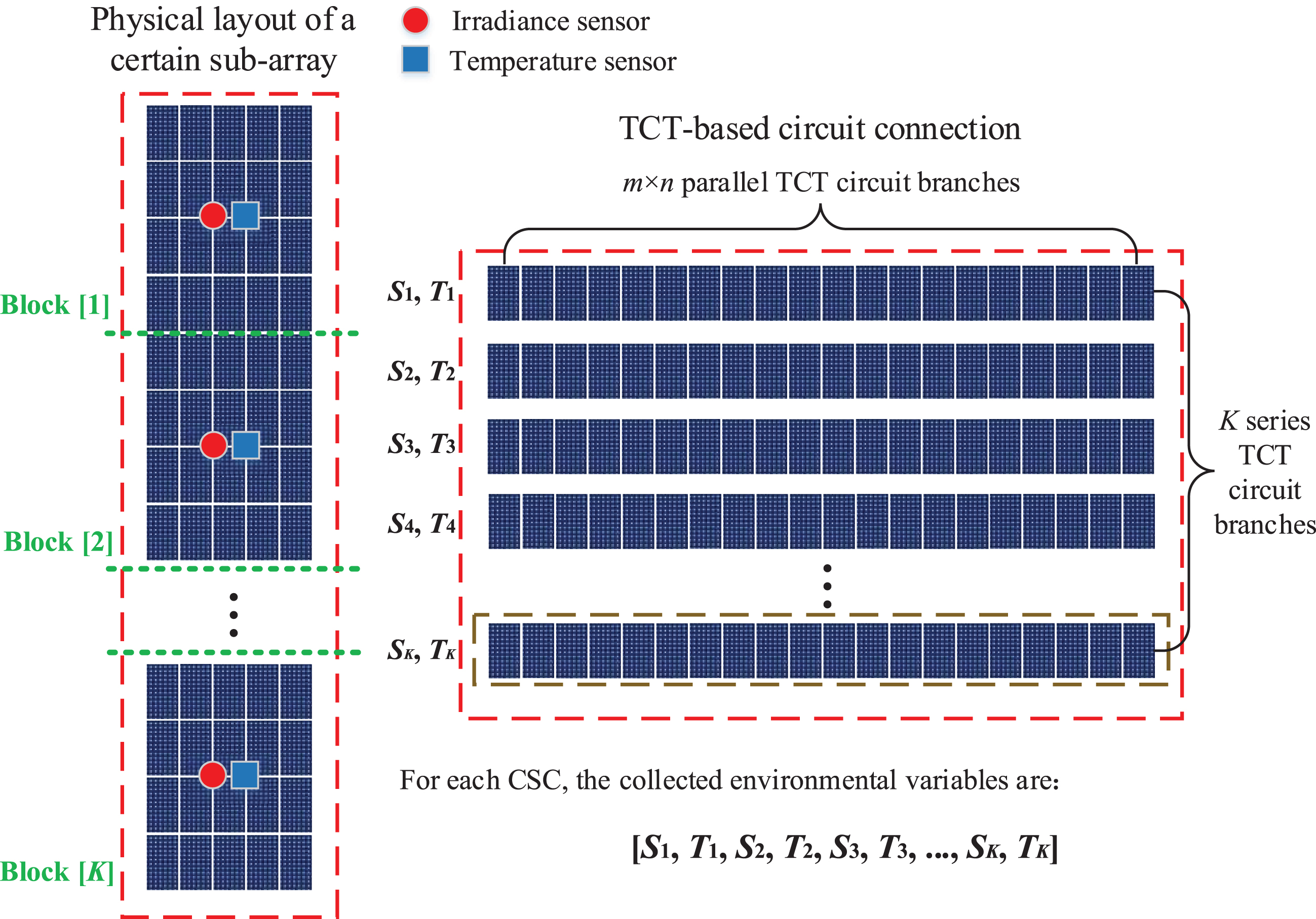
Environmental variables of BIPV sub-array in TCT configuration.
For a certain sub-array, the MPP under CSC entirely depends on all the collected environmental variables. In order to forecast the MPP under CSC/DSC accurately and quickly, the most direct way is to employ all the collected environmental variables (S1, S2, ... , S K , T1, T2, ... , T K ) as the model input, and the corresponding MPP voltage (V m ) is employed as the model output (denote as Model-I).
However, for a BIPV system installed on the facade of a super high-rise building, the system scale is always very large. As a result, the environmental variables may contain a lot of irradiance and temperature parameters, which will cause an increasing complexity of the ELM model. To overcome this problem, the collected environmental variables are firstly processed by feature extraction, then the obtained feature variables are employed as the model input (denote as Model-II). To be specific, the extracted feature variables contain the following four parts: The irradiance statistical variables: the maximum value of The temperature statistical variables: the maximum value of The local distribution variables of irradiance. Firstly, define four breakpoints as Q1 = S
min
+ (S
max
- S
min
)×20%; Q2 = S
min
+ (S
max
- S
min
)×40%; Q3=S
min
+ (S
max
- S
min
) ×60%; Q4=S
min
+ (S
max
- S
min
)×80%; Then, the local distribution variables of irradiance are defined as: the number of irradiances within the interval [S
min
Q1] (denote as NL1); the number of irradiances within the interval [Q1 Q2] (denote as NL2); the number of irradiances within the interval [Q2 Q3] (denote as NL3); the number of irradiances within the interval [Q3 Q4] (denote as NL4); the number of irradiances within the interval [Q4 S
max
] (denote as NL5). The global distribution variables of irradiance. Firstly, define four absolute irradiance breakpoints as QA1= 200 W/m2; QA2= 400 W/m2; QA3= 600 W/m2; QA4= 800 W/m2; Then, the global distribution variables of irradiance are defined as: the number of irradiances within the interval [0 QA1] (denote as NG1); the number of irradiances within the interval [QA1 QA2] (denote as NG2); the number of irradiances within the interval [QA2 QA3] (denote as NG3); the number of irradiances within the interval [QA3 QA4] (denote as NG4); the number of irradiances within the interval [QA4 +∞] (denote as NG5). The detailed input variables of Model-II are listed in Table 3.
Input variables of Model-II
Structures of the aforementioned MPPT models are illustrated as Fig. 9.

Structures of ELM-based fast MPPT model.
For the ELM-based MPPT model, an efficient training methodology with fast learning speed and high forecasting accuracy is necessary. Based on the basic theory of ELM, training methodology of the model is as follows:
Denote S sets of training samples as (
As the activation function is infinitely differentiable, the sample output can be approximated with zero error by ELM model theoretically, which is formulized as
Equation (2) can be rewritten as
According to the basic theory of extreme learning, all the linking weights ω and biases b are randomly generated. Then, the hidden layer output matrix H can be directly obtained using the following equation
Parameter settings
In this section, the proposed MPPT methodology for BIPV system is tested by simulation experiments. Parameters of the BIPV windows employed in the following experiments are set as: the short-circuit current under reference condition (I Scref ) is set to 12.2 A; the open-circuit voltage under reference (V Ocref ) is set to 21.7 V; the maximum power point current under reference condition (I mref ) is set to 11.1 A; the maximum power point voltage under reference condition (V mref ) is set to 18.1 V.
For the BIPV modules with the maximum system voltage of 1500 V, the evaluated BIPV array in the following experiments contains 75 blocks (i.e., K = 75 in Fig. 8), and each block contains 5×5 = 25 BIPV windows (i.e., m = n = 5 in Fig. 8). From the perspective of circuit connection, the evaluated BIPV array is a 75×25 TCT configuration which contains 75 series branches and each with 25 BIPV windows in parallel. The simulation environment is MATLAB R2019b.
Data generation
In order to verify the efficiency of ELM-based MPPT methodology, the sufficient training and forecasting samples are required, and these samples are generated using the numerical model of BIPV array. The engineering numerical model of basic PV module is adopted for data generation [40], which can be formulized as
For the evaluated 75×25 TCT-based BIPV array, randomly set the irradiance and temperature of each block, and generate 10000 sets of MPP samples under different CSC conditions. The MPP samples can be expressed as

Irradiances and temperatures of 5 random CSC samples.
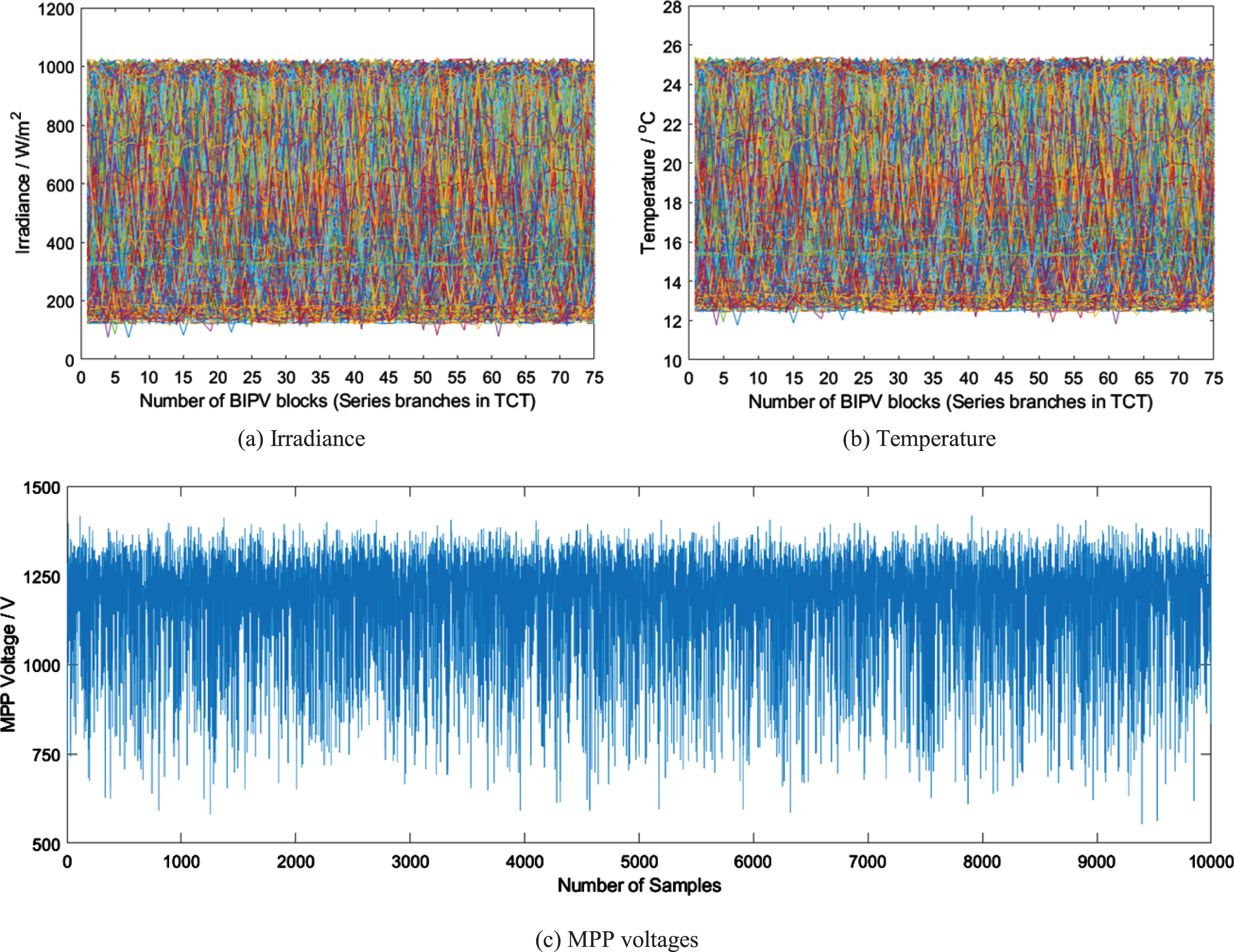
Irradiances, temperatures and MPP voltages of the entire 10000 CSC samples.
In this section, the proposed MPPT methodology is tested using the aforementioned 10000 MPP samples under CSC. The evaluated MPPT methodologies in case studies are as follows: (1) the ELM-based Model-I as described in Section 5.1 (denote as ELM-Model-I); (2) the ELM-based Model-II (denote as ELM-Model-II). In addition, the BP-ANN network is also employed for comparison: (3) BP-ANN using the input and output structures as in Model-I (denote as BP-Model-I); (4) BP-ANN using the structure as in Model-II (denote as BP-Model-II).
(1) Comparison of different MPPT methodologies
In the following case studies, randomly disorder the 10000 sets of CSC samples firstly. Then, employ the 9800 sets of samples to train each model, and employ the rest 200 sets as forecasting samples for testing. The optimal parameters of the investigated ELM-Model-I, ELM-Model-II, BP-Model-I and BP-Model-II are set as follows: for ELM-Model-I and ELM-Model-II, the hidden nodes number is set to 1000, the activation function is set to the sigmoid function; for BP-Model-I and BP-Model-II, the hidden layers number is set to 1, i.e., the classic single-hidden-layer structure is adopted in BP-based models. The hidden nodes number is set to 8, the activation function is set to the sigmoid function, the maximum iteration number is set to 20000. Outputs of ELM-Model-I, ELM-Model-II, BP-Model-I and BP-Model-II are compared in Fig. 12 and Table 4.
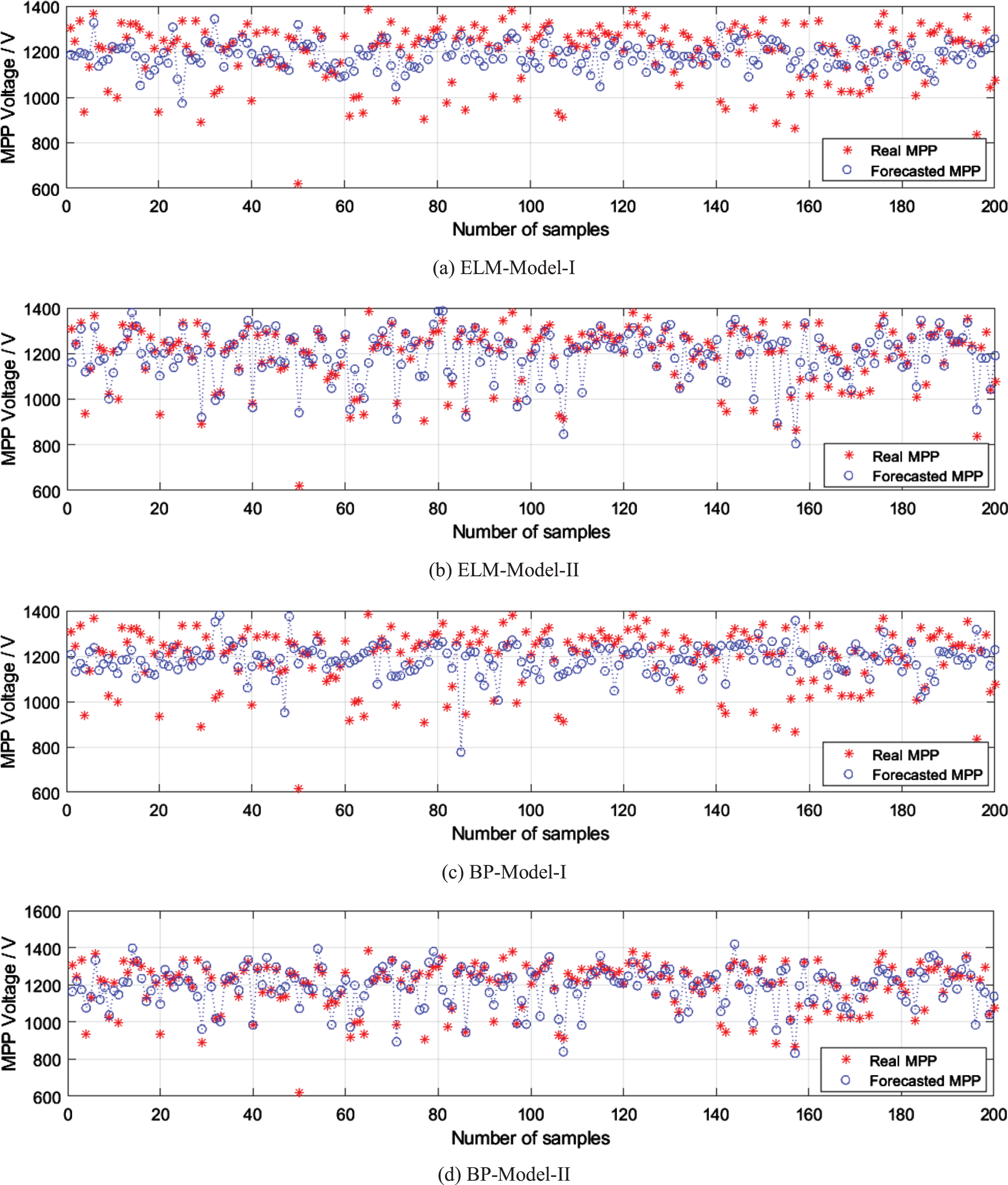
Forecasting of the 200 MPP samples.
Comparison of different methodologies on forecasting the 200 MPP samples
As shown in Fig. 12 and Table 4, the forecasting accuracy of ELM-Model-II and BP-Model-II is much better than that of ELM-Model-I and BP-Model-I. For example, the mean error of ELM-Model-II is 4.57%, which significantly outperforms 9.57% obtained by ELM-Model-I. In addition, the mean error of BP-Model-II is 5.07%, which also outperforms 9.84% obtained by BP-Model-I significantly. This implies that by extracting the feature variables listed in Table 3, the model can easily explore the relationship between the environmental variables and the corresponding MPP voltage. As a result, the model efficiency is significantly improved.
In terms of different training methodologies, the mean error of ELM-Model-II is 4.57%, which is slightly better than 5.07% obtained by BP-Model-II. Moreover, the time cost of ELM-Model-II is just 1.82 s, which is much faster than the BP-ANN-based models, e.g., 174.65 s obtained by ELM-Model-I, and 112.23 s obtained by ELM-Model-II. Note that because of the huge BIPV window quantity and unpredictable occupants’ behaviours, the CSC and DSC conditions are very common in BIPV system. As a result, the training and forecasting speed is very important for the MPPT control in BIPV application. As analysed above, comprehensively considering the forecasting accuracy and speed, the proposed ELM-Model-II performs the best.
(2) Comparison for more general cases
In order to further verify the outperformance and stability of ELM-Model-II, the comparisons for more general cases are conducted in this part. Specifically, the aforementioned 10000 MPP samples are repeatedly disordered. Then, the random 9900 samples are used to retrain each model, and the rest 100 samples are employed for forecasting tests. The comparisons are conducted for 5 different cases, and the experimental results are plotted in Fig. 13 and also summarized in Table 5. Note that in Table 5, the values outside and inside each bracket denote the mean forecasting error and the time cost, respectively. The last line in Table 5 denotes the average of Cases 1 to 5.
Comparisons for more general cases
As shown in Fig.13 and Table 5, the ELM-Model-II outperforms the compared methodologies for all the cases. To be specific, for Cases 1 to 5, the ELM and BP networks based on Model-II structure obtain higher forecasting accuracy compared with the Model-I based networks. This implies that to use the 20 parameters listed in Table 3 as the model input is useful for the CSC feature extraction, and this model structure is more efficient than directly employing all the environmental parameters as the model input. Moreover, by employing the ELM networks, the ELM-Model-II stably outperforms BP-Model-II on learning speed and forecasting accuracy. As discussed above, the proposed ELM-Model-II methodology is a good choice for the MPPT control of large BIPV system.
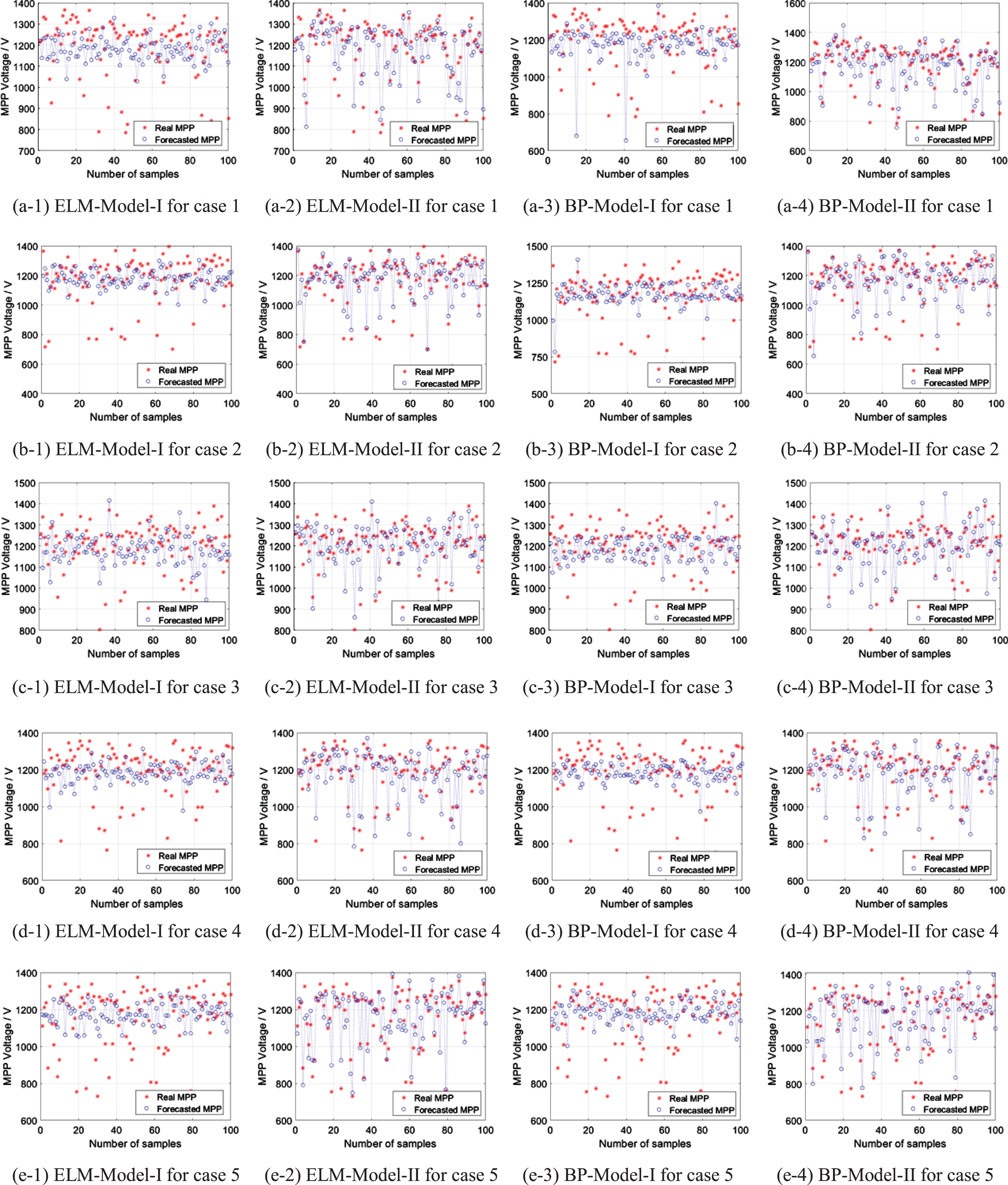
The forecasting curves for more general cases.
(3) Comparison for different scales of samples
In this part, the forecasting performance of ELM-Model-II on different scales of samples is further tested. First of all, generate 30000 sets of MPP samples use the method describes in Section 6.2. Then, employ the last 1000 samples as the testing samples, and the number of training samples increases from 1000 to 29000 step by step. The number of hidden nodes in ELM is set to 10% of the training sample number. For each scale of training samples, the independent forecasting tests are conducted for 10 times, and the average performance is used for evaluation. The experimental results are shown in Table 6.
Comparisons of ELM-Model-II for different sample scales
As shown in Table 6, the performance of ELM-Model-II is acceptable for the small scale of training samples. For example, the average forecasting errors are around 5% when the number of training samples is lower than 10000. In addition, it can be easily concluded from Table 6 that the performance of ELM-Model-II can be slightly improved with the increase of sample scale. Specifically, the average forecasting error approximately decreases from 5.51% to 4.31% when the sample number increases from 1000 to 29000.
Note that in the real application, the forecasting errors of ELM-Model-II can be furtherly eliminated by employing the online MPPT methodology as the second control step, for example, the P&O, InC and their variants [41-42]. On one hand, the online MPPT method can be regarded as the supplement to the offline ELM-Model-II for eliminating forecasting errors. On the other hand, the final output of online MPPT method can be employed as the newly generated training samples, and used for further training ELM-Model-II.
This study proposes an efficient PV array configuration and its fast MPPT methodology based on the extreme learning machine, in order to improve the performance of BIPV system under complex and dynamic shading conditions. First of all, some famous PV configurations are compared under complex shading conditions of BIPV system. Then, the best performer TCT-configuration is employed as the basic circuit connection unit, and the entire configuration of large-scale BIPV system installed on super high-rise building is proposed. Secondly, the input and output structures of data-driven MPPT network are described and two different model structures, i.e., Model-I (input all the environmental parameters) and Model-II (input twenty feature parameters), are proposed and compared. Then, in order to achieve promising performance on learning speed and forecasting accuracy, the extreme learning machine theory is employed for training the aforementioned MPPT models. Finally, the proposed ELM-Model-I, ELM-Model-II are tested and compared under a series of complex shading conditions, and the BP-ANN-based models, i.e., BP-Model-I and BP-Model-II, are also employed for comparison.
Experimental results show that the ELM-based models significantly outperform the BP-based models on learning speed, and the Model-II-based networks significantly outperform the Model-I-based networks on forecasting accuracy. As a result, the ELM-Model-II obtains the best performance for all the cases, and the average forecasting errors are just around 5%. Moreover, according to the experimental results, the ELM-Model-II can keep acceptable performance when the scale of training samples is small, and the forecasting error slightly decreases with the increase of training sample number.
In conclusion, the contribution of this study provides a novel methodology for the configuration design and operation control of large-scale BIPV system. The proposed methodology can ensure the maximum output power and fast response speed of BIPV system under complex and dynamic shading conditions, which are caused by the unpredictable behaviours of building’s occupants. However, there still exist some limitations in our study. For example, the prediction error is still large for some cases, in addition, the online MPPT step to cooperate with our offline model is not concerned in this study. In the future, more efforts could be made to further optimize the model structure and learning principles. On one hand, some further numerical experiments should be made to verify additional variables which affect the offline MPPT accuracy of TCT-based PV configuration. On the other hand, the latest achievements of ELM should be also concerned to further improve the prediction accuracy of our model. In addition, in the real engineering application of BIPV system, output of offline ELM model should be given to the online MPPT algorithm (e.g., the P&O, InC or their variants) as the control target, so the final performance is closely related to both the offline prediction part and the online control part. As a result, we will also consider the cooperation of data-driven MPPT network and the online MPPT control algorithm in our future work.
Conflict of interest
The authors declare that they have no conflict of interests regarding the publication of this paper.
Footnotes
Acknowledgments
This work was supported by the Fundamental Research Funds for the Central Universities (WUT: 2018IVB003).