An improved QPSO-SVM-based approach for predicting the milling force for white marble in robot stone machining

Abstract

Milling force prediction is one of the most important ways to improve the quality of products and stability in robot stone machining. In this paper, support vector machines (SVMs) are introduced to model the milling force of white marble, and the model parameters in the SVMs are optimized by the improved quantum-behaved particle swarm optimization (IQPSO) algorithm. A set of online inspection data from stone-machining robotic manipulators is adopted to train and test the model. The overall performance of the model is evaluated based on the decision coefficient (R2), mean absolute percentage error (MAPE) and root mean square error (RMSE), and the results obtained by IQPSO-SVM are superior to those of the PSO-SVM model. On this basis, the relationship between the milling force of white marble and various machining parameters is explored to obtain optimal machining parameters. The proposed model provides a tool for the adjustment of machining parameters to ensure stable machining quality. This approach is a new method and concept for milling force control and optimization research in the robotic stone milling process.

Keywords

Robot stone machining quantum-behaved particle swarm algorithm regression of support vector machines milling force of white marble machining parameters

1 Introduction

Because of their clear and crisp color and fine texture, white marble products are the highest value-added stone products among all three-dimensional carved stones. The application of industrial robots for the three-dimensional carving of white marble can make up for the shortcomings of traditional numerical control machining, such as the small working range, the inability to machine large and extremely large sculptures, and poor machining posture; thus, robots are the projected development direction in machining and three-dimensional stone carving [1]. Additionally, diamond cutting tools have been widely used in the field of white marble machining because of their long tool life and strong wear resistance [2]. However, due to the low stiffness of the robot structure and the hard brittle and natural crystal defects in white marble, the rock can easily break under a strong transient milling force (as shown in Fig. 1) [3]. Therefore, it is important to construct a prediction model of the milling force for white marble and establish the relationships between machining parameters and the milling force to guide the adjustment of machining parameters; the results provide an important reference for ensuring the stability of white marble carving with robots. It is difficult to precisely control the milling force of white marble due to the use of sophisticated equipment and complex control systems, as well as the extremely harsh working conditions; moreover, common prediction models of the milling force based on traditional mathematics cannot solve problems related to the strong coupling and nonlinearity among parameters. Therefore, the accuracy of milling force predictions for white marble is difficult to improve.

Fig. 1

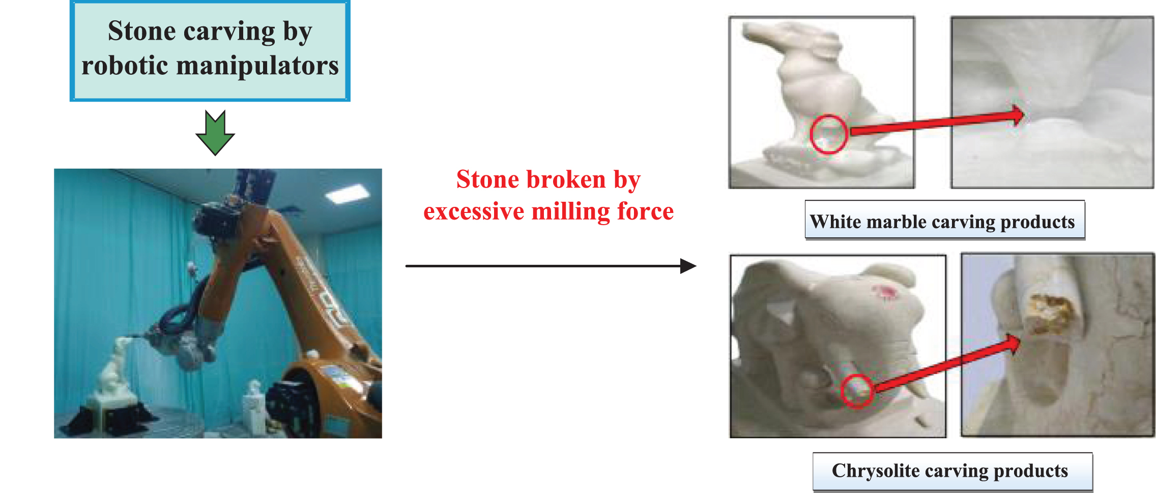
Breakage of white marble caused by an excessive milling force.

With the development of intelligent technology, many scholars have begun to introduce artificial neural network (ANN) methods into milling force models of the machining process [4, 5]. A prediction model for the milling force of a ball-end milling cutter was established by Zuperl using an ANN, and the prediction accuracy of the model reached 98% [6]. Hanafi et al. introduced an ANN method for the milling force prediction of TiC-coated tools in the process of milling PEEK CF30 material [7]. A prediction model of the milling force of Inconel 718 materials was established by Pawade based on grey relational analysis, and the effects of milling parameters on milling force output were explored [8]. Ratchev et al. established a neural network prediction model based on a genetic algorithm for complex thin-walled parts, and the error was less than 5% [9]. Cus et al. established a prediction mod el for white marble based on the use of TiC-coated tools considering the effects of the cutting speed, milling depth, tool geometry and material properties on the milling force [10]. Although ANNs have been widely used in the prediction of the milling force, they have problems such as a slow convergence speed and a long training time, and they often converge to a local optimal solution. In addition, ANNs adopt a training method of empirical risk minimization, which also limits the generalization ability of most networks [11, 12]. Research on artificial intelligence algorithms applied in milling force prediction for machine white marble has not been reported.

An SVM is a supervised machine learning model that is constructed based on the structural risk minimization criterion. Notably, compared with neural networks, SVMs can reduce the probability of overfitting based on an empirical risk minimization criterion, and the insensitive region in the structure can absorb the small-scale random fluctuations in a random response; thus, SVMs can be effectively applied in milling process prediction [13 –15]. The performance of an SVM model depends on the construction of the kernel function, and the selection of the parameters in the kernel function is the main problem in SVM applications. Generally, parameter selection methods can be divided into two categories. The first category includes grid search methods. In these methods, the step size for parameter change is set first, and each pair of parameter combinations is assessed to establish judgement function values; the whole parameter set space is searched, and the optimal value of the judgement function is retained [16]. This method can is most effective in cases with few parameters, but in practice, the calculation process is generally complex and time consuming. The other category of selection methods includes intelligent searching optimization algorithms such as the ant colony search (ACS) algorithm [17], genetic algorithm (GA) [18], and particle swarm optimization (PSO) algorithm [19]. The unique advantages and mechanisms of these algorithms have attracted the attention of the widespread attention of scholars [20 –22]. Notably, PSO is widely used in SVM parameter optimization because of its simple concept and fast convergence [23 –25].

This paper proposes a method for establishing a milling force model for the robot machining of white marble based on the IQPSO-SVM method. This approach overcomes the limitations of previous models for the modeling and optimization of the stone milling force based on actual data. Moreover, in practical problems, we use the IQPSO algorithm to optimize the parameters of the SVM, which improves the effectiveness of the SVM and reduces the control parameters of the traditional PSO algorithm. The core objective is to collect online data from the production process and then use it in practical production tasks after processing. The proposed model has the advantages of high pertinence and reliability.

This paper is organized as follows. In Section 2, the traditional model of the milling force of white marble is given, and the collection and processing of experimental data are briefly described. Section 3 describes the SVM theory. Section 4 introduces the basic PSO algorithm, and the SVM parameter optimization strategy based on IQPSO is proposed. In Section 5, the experimental results are analyzed and discussed, and compared with the PSO-SVM model, the superiority and accuracy of IQPSO-SVM are validated. In Section 6, the effects of machining parameters on the milling force modeling of white marble are determined. The conclusions are presented in Section

2 Definition of the milling force of white marble and the experimental database

2.1 Definition of the milling force of white marble

In the process of machining white marble, diamond milling cutters are used in a continuous grinding process. In addition to being subjected to the torsional force of the spindle, the diamond milling cutter is also subjected to the reaction force of white marble in the contact arc area, and the force will directly affect the service life of the milling cutter, the cutting performance of the diamond bit, the control characteristics of the matrix and the consumed power of the motor. These factors affect the machining quality and cost, which are extremely important to manufacturers. The force applied to white marble by a diamond milling cutter is distributed in the milling contact arc region. In this paper, the resultant force F_∑s is decomposed into a tangential milling force F_x, a radial milling force F_y and an axial milling force F_z (as shown in Fig. 2). It is assumed that the diamond particles are uniformly and continuously distributed on the arc surface of the milling cutter. The resultant force is decomposed in the x, y and z directions as follows:

${\begin{matrix} F_{x} = a_{p} \cdot F_{\sum} \cdot \int_{0}^{φ} sin (θ - β) d φ \\ F_{y} = a_{p} \cdot F_{\sum} \cdot \int_{0}^{φ} cos (θ - β) d φ \\ F_{z} = a_{p} \cdot F_{\sum} \cdot \int_{0}^{φ} cos (θ + β) d φ \end{matrix}$ (1)

where $φ = arccos (1 - a_{w} / l_{s})$ (2)

In this case, β is the angle between the normal force and resultant force of a single diamond particle, θ is the angle of the circular direction movement of the dynamic diamond particles along the contact arc of the tool, a_p is the axial cutting depth in the z direction, a_w is the radial cutting width in the y direction, and l_s is the contact length.

2.2 Traditional model for the milling force of white marble

For the milling of white marble with a diamond cutter, the theoretical formula for calculating the milling force is given based on the method in [26], which is shown as follows: $\begin{matrix} F_{Σ} = 2 a_{p} k_{t} \cdot \sqrt{{(1 + λ)}^{2}} \cdot \\ {[\frac{v_{f}}{v_{s}} \cdot \frac{1}{n_{d} \cdot ξ} \cdot {\frac{2 a_{w}}{d}}_{s} \cdot arccos (1 - 2 a_{w} / d_{s})]}^{\frac{α}{2}} \end{matrix}$ (3)

where v_f is relative feed rate of the milling cutter, v_s is the circular velocity of milling cutter, k_t is a constant, n_d is the dynamic effective grain number, λ is the milling force ratio, ξ is the cutting section coefficient, α is the coefficient of the average milling force, and d_s is the diameter of the cutter. Formula (3) indicates that most of the parameters in the theoretical formula of the milling force are related to the material properties of machined white marble and the cutter, which are nonlinear and difficult to confirm. It is difficult to predict the milling force for white marble with this formula in practice, so it is limited in practical applications. Notably, the parameters of the cutter when machining are important factors that can affect the milling force. The main goal of milling force prediction in white marble machining is to guide the optimization of machining parameters and improve the machining efficiency of cutters.

2.3 Experimental data acquisition and processing

A stone-carving robotic manipulator from a Stone Carving Company, which is located in Fujian Province, China, was used to collect experimental data and establish the prediction model of the stone milling force in this paper. We selected white marble as the studied stone, and the main components of white marble are quartz, feldspar and mica. White marble has a hard surface, so it is difficult to machine. The material removal rate must be high to quickly remove materials and maintain the profile of the model. Therefore, the machining process often produces a large milling force, which leads to tool wear and fractured products. There are two kinds of cutters used in white marble machining: diamond tools and carbide tools. White marble has high hardness and is difficult to machine, so diamond tools are most commonly used in white marble machining because of their high hardness and wear resistance. We selected an electroplated diamond wheel with 8 sections in this experiment. The tool parameters were as follows: the diameter was 50 mm, the height was 20 mm, the particle diameter was 465–561μm and the density was 271 particles/m³. The milling force date acquisition experiment was performed with stone-carving robotic manipulators, as shown in Fig. 2. The force measurement system consisted of a dynamometer, a signal amplifier, a data acquisition system and a computer. The basic principle is that the force signal in three directions (x, y and z) is measured by a dynamometer, transformed into an electrical signal, amplified by an amplifier and sent to a data acquisition system. Finally, a computer processes the data and obtains specific values. The experiment used a Kistler 9255B dynamometer, 5080 signal amplifier and DEWE high-speed data acquisition system, and the measuring process is shown in Fig. 3. The force acting on the workpiece during machining can be decomposed into forces in the x-axis, y-axis and z-axis directions. The tool feed direction along the positive y-axis is defined as F_x, the tool radial cutting direction along the positive x-axis is defined as F_y, and the force along the positive z-axis is defined as F_z.

Fig. 2

Force diagram for a milled stone.

Fig. 3

Test system for measuring the milling force of white marble and the tools used.

The technological parameters of white marble milling include the spindle speed n, feed speed f, cutting depth a_p and cutting width a_w. The section range of parameters is determined by combining existing equipment conditions with existing experience. The preliminary technological parameter ranges according to existing equipment conditions are as follows: the spindle speed n is 6000∼8000 r/min, the feed speed f is 4000∼6000 mm/min, the cutting depth a_p is 40% ∼50% of the cutter diameter, and the cutting width a_w is 1∼2 mm. Specific machining parameter values and the milling force measurement results are shown in Tables 1 and 2. There are 54 groups of milling force values based on different combinations of machining parameters, and we select the first 40 groups as the training set for the prediction model and the remaining 14 groups as the test set for the prediction model.

Table 1

Factors and level of experimental parameters for white marble milling

Factors	Level
	1	2	3
Spindle speed n (r/min)	6000	7000	8000
Feed speed f (mm/min)	4000	5000	6000
Cutting depth ap(mm)	0.4	0.8	1.2
Cutting width aw(mm)	0.4	0.5	0.6

Table 2

Measurement results for the milling force of white marble

Test no.	F_x(N)	F_y(N)	F_z(N)	Test no.	F_x(N)	F_y(N)	F_z(N)
1	23.132	39.578	175.47	28	55.659	125.887	350.06
2	19.388	42.465	180.23	29	42.017	91.586	423.98
3	–2.3132	40.872	220.31	30	15.087	98.187	445.32
4	5.6291	3.4561	140.23	31	35.232	65.973	338.11
5	–2.0882	31.253	142.76	32	40.052	52.373	381.58
6	–0.0781	53.232	219.87	33	45.272	68.978	385.22
7	7.8263	68.345	153.89	34	59.223	42.238	292.11
8	–3.0912	25.343	178.51	35	28.887	92.114	389.09
9	8.4268	25.909	208.23	36	42.132	71.22	381.97
10	11.231	17.832	219.38	37	81.887	172.54	401.93
11	–10.083	30.279	216.67	38	70.526	191.28	473.58
12	9.5225	26.371	305.45	39	59.278	169.44	537.83
13	14.522	40.878	231.43	40	69.558	182.34	396.21
14	19.331	8.4121	269.07	41	77.192	225.72	434.55
15	17.887	–15.231	289.19	42	92.031	242.78	468.89
16	13.445	4.7871	193.28	43	59.878	142.36	378.81
17	8.7872	45.381	258.79	44	55.637	149.38	448.09
18	12.334	31.191	296.83	45	77.699	166.03	498.77
19	39.676	98.131	256.13	46	110.23	212.86	456.63
20	15.466	88.421	327.85	47	125.11	169.07	481.05
21	6.8247	62.321	385.67	48	79.262	179.78	624.18
22	19.355	99.887	268.53	49	131.01	181.72	493.69
23	22.355	115.04	312.61	50	110.32	183.46	567.12
24	39.324	131.88	330.72	51	102.32	188.16	553.22
25	20.088	90.474	261.09	52	133.18	92.732	422.98
26	17.532	73.552	310.18	53	93.144	208.52	558.19
27	25.062	85.077	327.19	54	95.632	138.17	593.13

The training sample set and test sample set of the model fluctuate in different dimensions, as shown in Tables 1 and 2. To avoid model errors caused by data differences in different dimensions, it is necessary to rescale the data sets at certain intervals. The normalized mapping method was applied based on the following formula: $x_{i}^{'} = \frac{x_{i} - \min (x_{i})}{\max (x_{i}) - \min (x_{i})}, i = 1, 2, 3, \dots, n$ (4) where max(x_i) is the maximum value in a data set and min(x_i) is the minimum value in the data set.

3 Support vector machine method

3.1 Support vector regression theory

In view of the complexity and stochastic volatility of the milling process and the high cost of obtaining experimental data, we used an SVM method, which has distinct advantages in dealing with a small sample size and nonlinear relations, to construct the milling force prediction model for white marble. In white marble processing, the input variables x_i = [v_f,i,v_s,i,a_p,i,a_w,i] and the output variables F_i = [F_x,i,F_y,i,F_z,i] of each set of experiments form the sample space {(x_i,F_i),i = 1,2,3, ... ,n}. ɛ-support vector regression (ɛ-SVR) is commonly used to solve regression problems. In ɛ-SVR, the deviation between the output f_F(x) of the regression prediction and the real output F_i must be less than ɛ, and a range with a width of 2ɛ is established at the center of f_F (x). A result is considered satisfactory if it falls within this range. f_F (x) can be expressed as a nonlinear function, as shown in formula (5): $f_{F} (x) = ω^{T} φ (x) + b$ (5) where φ(x) is the nonlinear mapping of input space x, ω is the linear form of φ(x), b is the bias, and ω and b can be determined from formula (2). $\min_{ω, b} (\frac{1}{2} {∥ ω ∥}^{2} + C \sum_{i = 1}^{n} l_{ɛ} (f_{F} (x_{i}) - F_{i}))$ (6) where C is the penalty factor (C > 0) and lɛ is the loss function, which can be calculated as follows: $l_{ɛ} (τ) = {\begin{matrix} 0, if | τ | ⩽ ɛ \\ | τ | - ɛ, otherwise \end{matrix}$ (7)

We introduce relaxation factors ξ_i ⩾ 0 and $ξ_{i}^{*} ⩾ 0$ because of the existence of fitting errors. Now, the optimization objective can be changed as follows: $\begin{matrix} \min_{ω, b, ξ, ξ^{*}} (\frac{1}{2} ω^{T} ω + C \sum_{i = 1}^{n} (ξ_{i} + ξ_{i}^{*})) \\ s . t . f_{F} (x_{i}) - F_{i} ⩽ ɛ + ξ_{i} \\ F_{i} - f_{F} (x_{i}) ⩽ ɛ + ξ_{i}^{*} \\ ξ_{i}, ξ_{i}^{*} ⩾ 0, i = 1, \dots, n . \end{matrix}$ (8)

The Lagrange equation is established by introducing Lagrange multipliers as follows:

$\begin{matrix} L (ω, b, ξ, ξ^{*}, α, α^{*}, η, η^{*}) = \\ \frac{1}{2} ω^{T} ω + C \sum_{i = 1}^{n} (ξ_{i} + ξ_{i}^{*}) - \sum_{i = 1}^{n} (η_{i} ξ_{i} + η_{i}^{*} ξ_{i}^{*}) \end{matrix}$ $\begin{matrix} - \sum_{i = 1}^{n} α_{i} [ɛ + ξ_{i} - F_{i} + ω^{T} φ (x_{i}) + b] \\ - \sum_{i = 1}^{n} α_{i}^{*} [ɛ + ξ_{i}^{*} - F_{i} + ω^{T} φ (x_{i}) + b] \end{matrix}$ (9) where α,,α^*, η and η^* are the Lagrange multipliers. The optimal conditions are as follows: ${\begin{matrix} \frac{\partial L}{\partial ω} = 0 \Rightarrow ω = \sum_{i = 1}^{n} (α_{i}^{*} - α_{i}) x_{i} \\ \frac{\partial L}{\partial b} = 0 \Rightarrow 0 = \sum_{i = 1}^{n} (α_{i}^{*} - α_{i}) \\ \frac{\partial L}{\partial ξ_{i}} = 0 \Rightarrow C = α_{i} + η_{i} \\ \frac{\partial L}{\partial ξ_{i}^{*}} = 0 \Rightarrow C = α_{i}^{*} + η_{i}^{*} \end{matrix}$ (10)

After eliminating ω,b,ξ, ξ^*,η and η^*, duality theory can be used to solve the SVR problem by converting it to a quadratic programming problem. By substituting formula (10) into the Lagrange equation, we obtain the following formula: $\begin{matrix} \max_{α, α^{*}} \sum_{i = 1}^{n} F_{i} (α_{i} - α_{i}^{*}) - ɛ (α_{i}^{*} + α_{i}) \\ - \frac{1}{2} \sum_{i = 1}^{n} \sum_{j = 1}^{n} {(α_{i} - α_{i}^{*})}^{T} (α_{i} - α_{i}^{*}) x_{i}^{T} x_{j} \\ s . t . \sum_{i = 1}^{n} (α_{i} - α_{i}^{*}) = 0 \\ α_{i}, α_{i}^{*} \in [0, C] \end{matrix}$ (11)

The above process satisfies the Karush-Kuhn-Tucker (KKT) conditions: ${\begin{matrix} α_{i} [f_{F} (x_{i}) - F_{i} - ɛ - ξ_{i}] = 0 \\ α_{i}^{*} [F_{i} - f_{F} (x_{i}) - ɛ - ξ_{i}^{*}] = 0 \\ α_{i} α_{i}^{*} = 0, ξ_{i} ξ_{i}^{*} = 0 \\ (C - α_{i}) ξ_{i} = 0, (C - α_{i}^{*}) ξ_{i}^{*} = 0 \end{matrix}$ (12)

Formula (11) can be solved to obtain the regression function of ɛ-SVR as follows: $f_{F} (x) = \sum_{i = 1}^{n} (α_{i}^{*} - α_{i}) K (x_{i}, x_{j}) + b$ (13) where K(x_i,x_j) =φ(x_i)φ(x_j), which is a kernel function. The feature spaces mapped by different kernel functions are also highly different. The Gao Si radial basis function (RBF), which is characterized by high adaptability, is selected as the kernel function in this paper, as shown in formula (14): $K (x_{i}, x_{j}) = \exp (- \frac{∥ x_{i} - x_{j} ∥}{2 σ^{2}})$ (14) where σ is the width of the kernel function.

3.2 Parameters of the SVR model

The parameter σ in the RBF kernel function and penalty factor C effect the prediction performance of the model in practical problems such as milling force prediction for white marble with an SVM. The penalty factor C is the degree of punishment for the training model for incorrectly allocating samples, and it is used to adjust the experience risk and confidence interval of the learning model to ensure that the training model has high generalization ability. A small penalty factor C reflects a small punishment degree for empirical errors in milling force prediction for white marble; a learning machine may be easier to use, but the empirical risk increases. The empirical risk and generalization ability of the trained model will be stable in the state of overlearning when the penalty factor C is large.

The change in σ in the RBF kernel function is actually an implicit change in the mapping function that affects the magnitude of structural risk after the mapping function changes. σ controls the effect of regression fitting with the SVM and influences the number of SVMs that should be used and the generalization ability of the training model. The larger σ is, the smaller the number of SVMs in the model and lower the accuracy of the regression prediction. The smaller σ is, the higher the accuracy of regression prediction, but the generalization ability of the model may be poor when many SVMs are used. Thus, for each specific problem, optimal values of the penalty factor C and parameter σ must be determined to ensure that the model has satisfactory generalization ability and high prediction accuracy. The PSO algorithm is an efficient global optimization algorithm that can effectively select the best combination of internal parameters for an SVM model and improve the prediction accuracy and generalization ability of the model. The traditional PSO algorithm and IQPSO algorithm are used to optimize the penalty factor C and parameter σ and obtain satisfactory parameters for the SVMs.

4 Optimization of SVR with IQPSO

4.1 Basic PSO algorithm

Eberhart and Kennedy proposed the initial PSO algorithm, which involved particle movement in the solution space toward the optimal solution; the intelligence and social properties of the model ensure that particles land at the optimal solution without landing elsewhere. The PSO algorithm assumes that the possible solution of the problem is a point in the n-dimensional search space, and “particles” are used to search this space. Particles fly in the search space at a certain speed and dynamically adjust their flight according to their own flight experience and the experiences of other particles. Each particle uses their current position, their current speed, the distance between their current position and that of the best particle, and the distance between their current position and that of the global best particle to change their course. Optimizing the search process is an iterative procedure in which a group of randomly initialized particles evolve and share information in the population.

The basic objective of the PSO algorithm is to accelerate each particle to the best position. The starting positions and velocities of the particles are randomly set in the solution space. The algorithm will record the best position and corresponding fitness function values of each single particle and the group of particles. The specific mathematical description is as follows. Assuming that the search space for particles is n-dimensional, the whole particle swarm includes N particles, and the position of particle i is X_i = [x_i₁,x_i2,x_i₃, ... ,x_iN]^T; additionally, the velocity of particle i is V_i = [v_i₁,v_i₂,v_i₃, ... ,v_i_N]^T. The individual extremum of particle i is P_i = [p_i₁,p_i₂,p_i₃, ... ,p_i_N]^T, and the global extremum of the group is P_g = [p_g₁,p_g₂,p_g₃, ... ,p_gN]^T. When a particle finds the best individual or global position, it can update its velocity and position information according to formula (15) and formula (16). $V_{id}^{t + 1} = ω V_{id}^{t} + c_{1} r_{1} (P_{id}^{t} - X_{id}^{t}) + c_{2} r_{2} (P_{gd}^{t} - X_{id}^{t})$ (15) $X_{id}^{t + 1} = X_{id}^{t} + V_{id}^{t + 1}$ (16) where ω is the inertial weight, which is used to adjust the velocity of each particle; c₁ and c₂ are learning factors; r₁ and r₂ are used to produce random numbers between 0 and 1; $V_{id}^{t}$ and $X_{id}^{t}$ are the velocity and position of particle i in dimension d at iteration t, respectively; $P_{id}^{t}$ is the individual extremum position of a single particle, $P_{gd}^{t}$ is the global extremum position of the group, and t is the number of cycles (t = 1, 2, ...). The stopping condition for the iterative process can be set according to the specific problem considered and is usually set based on the maximum number of iterations K or the time at which the optimal location is determined in the group search. The standard 2011 PSO algorithm is used in this paper; it involves some improvements over the traditional method [27, 28, 27, 28], and the basic PSO parameters are set as shown in Table 3.

Table 3

The parameters used in PSO

Parameters	Values
Size of populations N	40
Inertial weight ω	$\frac{1}{5 ln 3}$
Acceleration factors c₁ and c₂	ln 3 +0.7
Number of iterations K	150

4.2 PSO with improved quantum behavior (IQPSO)

In the traditional PSO algorithm, each iteration uses only the global and individual optimal information without fully using the information obtained in the calculation process, which can easily lead to a slow convergence speed and low search accuracy [29, 30]. The QPSO algorithm subverts the regeneration method of the traditional particle swarm algorithm, requires fewer parameters than the PSO algorithm, and has a stronger global search ability than the standard PSO algorithm [31, 32]. This paper improves the updating formula of the only contraction-expansion factor that needs to be adjusted in the QPSO algorithm and introduces the differential evolution operator. Combining the two methods gives a self-improved quantum particle swarm optimization (IQPSO) algorithm and improves the updating formula of the contraction-expansion coefficient according to the different demands of the algorithm for the contraction-expansion factor in the early and late calculation stages. Moreover, the differential evolution operation is added to the search group with a certain probability in the particle search process, thus increasing the randomness of the particles and reducing the probability of the particles falling to a local optimum to improve the global search ability of the algorithm.

In the QPSO algorithm, the particle swarm is updated and evolves according to the following formula: $P_{jd} = φ \cdot P_{id} + (1 - φ) \cdot P_{gd}$ (17) $lbest = (\frac{1}{L} \sum_{i = 1}^{L} P_{i 1}, \frac{1}{L} \sum_{i = 1}^{L} P_{i 2}, \dots, \frac{1}{L} \sum_{i = 1}^{L} P_{id})$ (18) $X_{id} = P_{jd} \pm α \cdot | {lbest}_{id} - X_{id} | \cdot ln (1 / u)$ (19) where φ is a random number between 0 and 1, P_jd is a random position between P_id and P_gd, lbest is the neutral position of the particle swarm P_id, and α is the contraction-expansion coefficient of QPSO.

The selection of the contraction-expansion coefficient α has a large influence on the convergence speed and accuracy of the QPSO algorithm. A small α is beneficial to local searching, but the algorithm converges slowly; a large α is beneficial to global searching, and the algorithm converges quickly, but accurate solutions are difficult to obtain. Conventional calculation formulas for α are monotonically decreasing linear functions (as shown in formula (20)), and with these formulas, it is difficult to meet the demands for flexible and dynamic changes the in contraction-expansion factors. $α (t) = α_{m} + \frac{(α_{0} - α_{m}) (T - t)}{T}$ (20) where α₀ and α _m are the initial and final values of the contraction and expansion coefficients, respectively.

The particle aggregation degree k(t) indicates the degree to which particles aggregate at a specific location or at several specific locations, which can effectively reflect the iterative period of the algorithm. k(t) is regarded as an important basis for the dynamic adjust of α in this paper, and the specific formula is: $k (t) = P_{g} (t) / {avgP}_{i} (t)$ (21)

On the basis of the particle aggregation degree k(t), the formula for the contraction-expansion coefficient α _IQ in the IQPSO algorithm is: $α_{IQ} (t) = (α_{0} - α_{m}) \cdot exp [- {(t / T)}^{2} \cdot k (t)] + α_{m}$ (22)

Formula (17) and formula (19) can be used to obtain:

$\begin{matrix} X_{id} = φ \cdot (P_{id} - P_{gd}) + P_{gd} \pm α_{IQ} \cdot | {lbest}_{d} \\ - X_{id} | \cdot ln (1 / u) \end{matrix}$ (23)

Formula (23) shows that when the current position X_id of a particle, the individual optimal position P_id and the global optimal position P_gd are very close in the search process, the first term (P_id -P_gd) in the above formula will cause the updating formula to fail, lead to the loss of the diversity in the particle swarm and increase the probability of the group falling to a local optimal position.

The differential evolution operator λ _jk between particle j and particle k can be obtained by randomly selecting two particles at different positions for any particle i in the current particle swarm. The corresponding formula is shown as follows: $λ_{jk} = X_{k} - X_{j}$ (24)

By substituting formula (24) into formula (23) and adding a random number between 0 and 1 to increase randomness, the evolutionary process of the IQPSO algorithm is obtained as follows:

$\begin{matrix} X_{id} = φ \cdot λ_{d} + (1 - φ) \cdot P_{gd} \\ \pm α_{IQ} \cdot | {lbest}_{d} - X_{id} | \cdot ln (1 / u) \end{matrix}$ (25)

Formula (25) shows that the introduction of the differential evolution operator λ will avoid a reduction in diversity in the group and trapping at local optima, and the improved contraction-expansion coefficient α _IQ strengthens the search performance of the algorithm in iterative calculations in each period.

The standard PSO algorithm, the standard QPSO algorithm and the IQPSO algorithm are used to compare the minimum values obtained with four commonly used test functions. The test function is shown in Table 4, and the minimum value of the test function is zero. The test data dimension is set to 20 and 40, and the number of iterations is 2000 and 4000. The average value (F_avg) and standard deviation (F_SD) of each the simulations of each algorithm are shown in Table 5.

Table 4

Benchmark functions and settings

	Test function	Initialization range	Search scope
Schwefel	$f (x) = 419 - \sum_{i = 1}^{d} x_{i} sin (\sqrt{\| x_{i} \|})$	(50, 100)	(–100, 100)
Gramacy	$f (x) = \frac{sin (10 π x_{i})}{2 x} + {(x_{i} - 1)}^{4}$	(20, 35)	(–60, 60)
Michalewicz	$f (x) = - \sum_{i = 1}^{d} sin (x_{i}) {sin}^{2 m} (\frac{{ix}_{i}^{2}}{π})$	(1.87, 4.36)	(–6.38, 6.38)
Zakharov	$f (x) = \sum_{i = 1}^{d} x_{i}^{2} + {(\sum_{i = 1}^{d} 0.5 {ix}_{i})}^{2} + {(\sum_{i = 1}^{d} 0.5 {ix}_{i})}^{4}$	(–10, 10)	(–20, 20)

Table 5

Numerical comparison of the test functions

Test function	Schwefel		Gramacy		Michalewicz		Zakharov
Dimension	20	40	20	40	20	40	20	40
Iteration times	2000	4000	2000	4000	2000	4000	2000	4000
PSO-F_avg	5.38e-27	1.36e-12	18.1034	138.434	2.59e-15	1.73e-14	6.8752	17.8692
QPSO-F_avg	4.89e-68	2.11e-43	13.4568	52.3268	8.78e-18	4.38e-18	4.2837	12.2365
IQPSO-F_avg	6.94e-98	2.42e-82	7.82567	15.4258	6.37e-18	1.49e-18	0.0023	0.00671
PSO-F_SD	4.32e-13	3.27e-13	32.7037	37.4235	9.88e-6	4.582e-5	4.2352	8.5369
QPSO-F_SD	3.87e-65	1.36e-43	31.5269	35.6987	3.22e-19	4.88e-18	2.3244	1.8226
IQPSO-F_SD	5.77e-95	1.11e-82	0.32589	0.34579	1.37e-19	1.02e-18	0.0007	0.0002

Table 5 indicates that the IQPSO algorithm yields the smallest value for all test functions. The IQPSO algorithm has better local search accuracy than the standard QPSO algorithm and PSO algorithm for the Schwefel function, which suggests that the improved algorithm can effectively promote local convergence. For the Gramacy function, IQPSO yields a better objective function value than do the other algorithms, and the standard deviation is smaller, which reflects the superior global search ability and global convergence ability of the proposed method.

4.3 Strategy of IQPSO with SVR

The SVM prediction model for parameter optimization includes three parts: range determination for the optimization parameters, the selection of a fitness function and algorithm implementation. First, the search ranges of parameters are determined, and the effective search space is defined to reduce the search time. We obtain the estimated value of C based on the target value expression. Then, by taking the calculated value of C and 50% of the average value of the target variable to establish a normal distribution of values, two points on both sides of the estimated value C are selected to determine the range of C, as shown in formula (26). The specific expression of the search range of parameter σ is shown in formula (27) [33]. $C = max (| F_{avg} + 3 F_{SD} |, | F_{avg} - 3 F_{SD} |)$ (26) $σ = [0 . 1^{1 / z}, 0 . 5^{1 / z}]$ (27) where Z is the number of parameters that have an important influence on the experimental process; for the white marble milling experiment in this paper, z = 4, and the milling speed, milling depth, milling width and feed speed are particularly important.

Second, because the SVM can reduce the generalization error of the model, this paper selects the mean square error (MSE) as the fitness function; that is, the MSE of the model output is minimized as the target of optimizing C and σ, as shown in formula (28). $MSE = \frac{\sum_{i = 1}^{n} {| F_{i} - F_{i}^{*} |}^{2}}{n}$ (28) where F _i is the measured milling force value for white marble and F* i is the predicted milling force value for white marble.

Finally, 50 sets of training sets are used to train the IQPSO-SVM model, and the optimal combination of C and σ values that satisfy the fitness function (minimum MSE) is iteratively obtained. The optimization is complete when the predefined maximum number of iterations is exceeded. The process of searching for the best intrinsic parameters is shown in Fig. 4.

Fig. 4

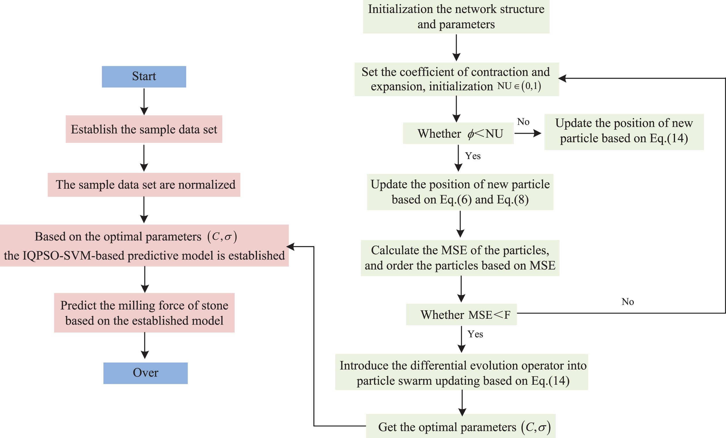
Flow chart for optimizing the SVM parameters (C, σ) by IQPSO.

Step 1. Set the parameters of the IQPSO algorithm, such as the particle group size, number of iteration cycles and sample dimension, to initialize the particle group. The initial fitness is used to evaluate the quality of each particle in the particle group and to update the position and velocity of the current particle.

Step 2. Set the contraction-expansion coefficient α _IQ , initialize NU∈(0,1), and update the average neutral position of the particles in the group according to formula (18).

Step 3. Randomly select a numerical value φ between 0 and 1 to confirm whether φ is less than NU. If φ is less than NU, update the particle position according to formula (17) and formula (19); otherwise, update the particle position according to formula (25).

Step 4. Calculate the fitness variance of the group according to formula (28) to determine whether the MSE is less than a given threshold F; if so, a differential evolution operator is introduced to update the particle group according to formula (25). Then, the process returns to Step 1.

Step 5. Export the individual fitness value and optimal position of the particle, extract the optimal parameters (C, σ) of the SVM after the iterative operation, and build the SVM algorithm based on IQPSO.

Step 6. During the early preprocessing of data samples, the correlation function of the SVM is used to normalize the selected samples and convert them to real numbers between 0 and 1.

Step 7. Use the SVM algorithm to determine the intrusion behavior of the training data sample set, which is selected in the beginning of the process, and statistically analyze the data for samples in the network based on the IQPSO-SVM model established by training. Finally, the forecasting results are output by the model. normalize the selected samples and convert them to real numbers between 0 and 1.

5 Experimental results and analysis

5.1 Performance criteria

A performance index can reflect the quality of a model and the fitting degree between the output of the model and actual measured values. In this paper, we use MSE, MAPE and R² as the indexes to evaluate the predictive performance of the model. The smaller the prediction error of the evaluation data is based on the MSE, the better the result; the MSE is expressed as shown in formula (28). The MAPE (shown in formula (29)) is a measure of predictive accuracy in the field of statistics; it is a relative value that can measure the prediction effect of multiple different models based on the same data. The smaller the MAPE is, the higher the prediction accuracy of the model is. The model result is perfect when the MAPE is 0% and extremely poor when the MAPE is greater than 100%. R² is the ratio of the sum of the squared regression values at observation points to the sum of squares from multiple regression, as shown in formula (30). This statistic measures the fitting degree for a multiple regression equation and reflects the ratio of the result explained by the estimated regression equation in the variation of dependent variable y. Generally, the closer R² is to 1, the greater the ratio of the sum of the regression squares of the observation points to the sum of the total squares. The closer the regression line is to each observation point, the better the fitting degree of the observation point regression. Thus, the better the interpretation of the dependent variables is based on the independent variables in the regression analysis, the better the prediction effect of the model. $MAPE = \frac{\sum_{i = 1}^{n} {| \frac{F_{i} - F_{i}^{*}}{F_{i}} |}^{2}}{n} \times 100$ (29) $R^{2} = 1 - \frac{\sum_{i = 1}^{n} {(F_{i} - F_{i}^{*})}^{2}}{\sum_{i = 1}^{n} {(F_{i} - \frac{1}{n} \sum_{i = 1}^{n} F_{i})}^{2}} \times 100 %$ (30)

5.2 Effect of parameter (C, σ) combinations on the model results

The analysis in Section 3.2 indicates that the C and σ values have an important influence on the prediction accuracy of the model when the support vector machine method is used to establish the prediction model of the milling force for white marble. With a focus on the effects of C and σ on the model prediction accuracy, based on the experimental data obtained in Section 2.3, a grid search method with three cross-validation steps is used to plot the variation in the performance index MSE when C and σ change, as shown in Fig. 5. Figure 5 shows that multiple combinations of C and σ can minimize the MSE. Compared with the grid search algorithm, the particle swarm algorithm does not have to traverse all the points in the grid, and it can find the global optimal solution; thus, it is simple and saves time. Therefore, in this paper, we use the QPSO algorithm and IQPSO algorithm to search for the optimal combination of (C, σ), and the search results are shown in Table 6.

Fig. 5

Model prediction error with (C, σ) changes: (a) F_x ; (b) F_y; and (c) F_z.

Table 6

The best C and σ values from the prediction model

Predicted F /N Models\Models	C by IQPSO	C by QPSO	σ by IQPSO	σ by QPSO
	SVM	SVM	SVM	SVM
_Fx	4.2871	1.3871	1.5157	1.6532
_Fy	0.2679	0.1324	0.5359	0.7883
_Fz	8.0312	4.3257	0.0442	0.0588

5.3 Comparison of different optimization algorithms

A prediction model of the milling force for white marble based on QPSO-SVM and IQPSO-SVM is established, and the fitting degree of the two models is qualitatively analyzed by linear fitting regression analysis of the predicted and actual values. The closer the fitting curve is to the optimal curve y = x, the smaller the discrete degree of scatter and the better the regression effect or prediction effect is. We use the F value to evaluate this result. A test (variance analysis) for F in the prediction model is used to determine whether the parameters in the model are suitable for estimation with data in a given range outside the training set and test set. Calculate the F value and the probability P (F > Fa) value, where P > 0.1 indicates that the model factor has little influence on the model output and P < 0.05 indicates that the model factor has a significant influence on the output. F is verified by testing to determine whether the model is considered effective. The F values of different models based on the same data will vary. If F values are all qualified by testing, the larger F is, the closer the corresponding model is to the ideal model, that is, the smaller the gap between the fitting curve and the optimal y = x curve is. QPSO-SVM and IQPSO-SVM are used to analyze the predicted and actual values based on the training set and test set; the fitting results are shown in Figs. 6 and 7, and the F and P test results are shown in Table 7.

Fig. 6

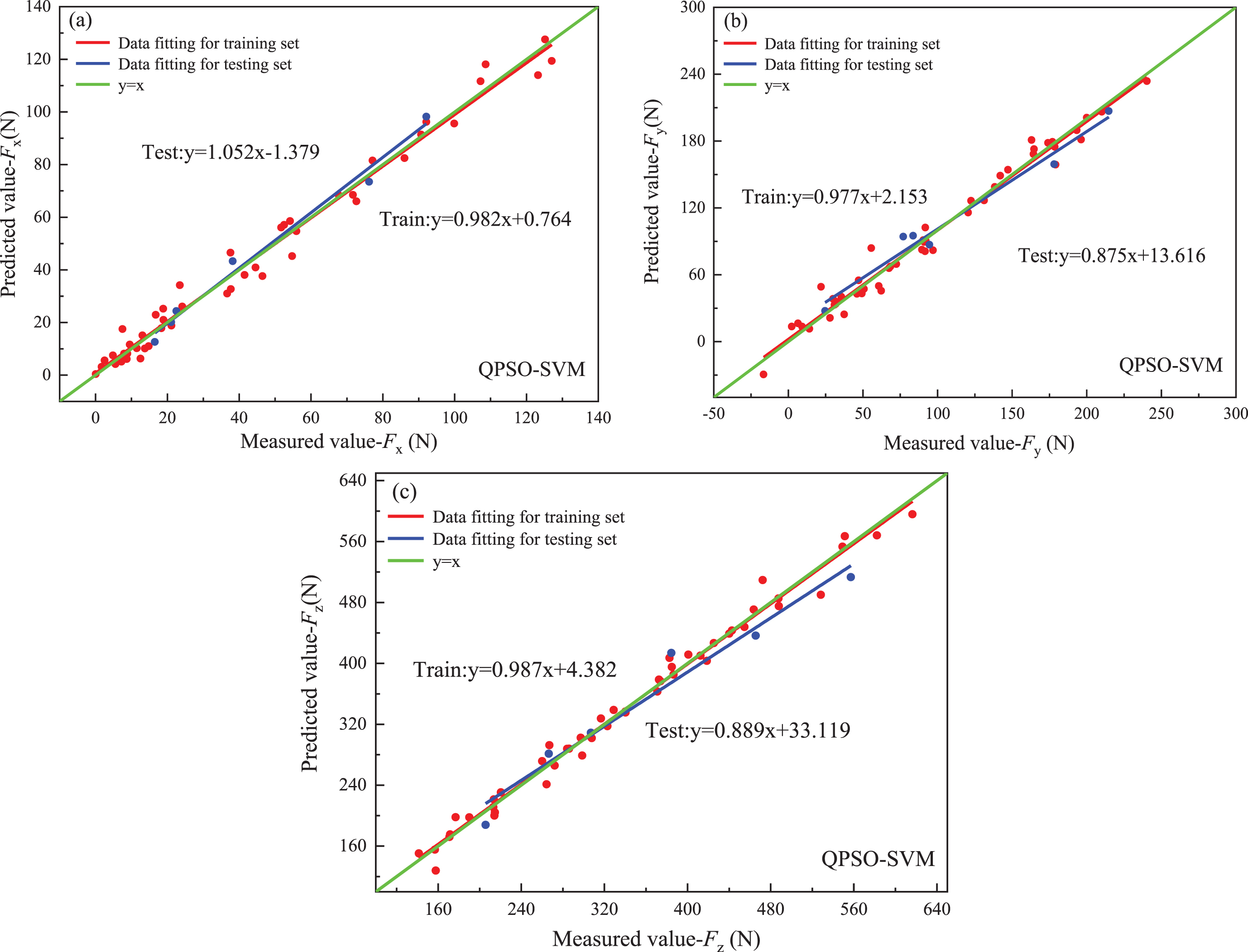
Linear fitting analysis of force F of white marble milling based on QPSO-SVM: (a) F_x ; (b) F_y; and (c) F_z.

Fig. 7

Linear fitting analysis of the force F of marble milling based on IQPSO-SVM: (a) F_x ; (b) F_y; and (c) F_z.

Table 7

F and P test results for the IQPSO-SVM model and QPSO-SVM model

Predicted F /N\Index	F by	F by	P by	P by
	IQPSO-SVM	QPSO-SVM	IQPSO-SVM	QPSO-SVM
F_x-train	75.285	63.294	2.93e-5	5.69e-5
F_x-test	70.283	53.075	3.91e-5	6.79e-5
F_y-train	43.296	41.804	9.76e-5	1.01e-4
F_y-test	30.197	28.408	1.18e-4	2.67e-4
F_z-train	77.185	74.304	2.32e-5	3.05e-5
F_z-test	75.737	16.320	2.68e-5	5.85e-4

According to the above linear fitting and test results, both QPSO-SVM and IQPSO-SVM are effective in predicting the milling force F_x of white marble. However, by comparing the F values in the table, we can find that the F values of the training set and the test set based on the IQPSO-SVM model are larger than the F values of the QPSO-SVM model; in other words, the regression effect and prediction effect of the IQPSO-SVM model are better than those of the QPSO-SVM model. For F_y and F_z, the same conclusion can be clearly obtained by comparing the QPSO-SVM model fitting analysis diagram and the IQPSO-SVM model fitting analysis diagram. The regression and prediction results are generally similar, which indicates that the IQPSO-SVM model has satisfactory generalization ability.

Second, the prediction model of the milling force for white marble was assessed based on the QPSO-SVM and IQPSO-SVM algorithms. The prediction curves of F_x, F_y and F_z obtained by the two models are shown in Fig. 8, and the prediction result for each prediction model and corresponding relative error are shown in Table 8.

Fig. 8

Model prediction curve and actual curve for QPSO-SVM and IQPSO-SVM: (a) F_x; (b) F_y; and (c) F_z.

Table 8(a)

Prediction result for each prediction model and the corresponding relative error for Fx

Number	n	f	a_w	a _p	Measured	Predicted F_x (N)		Error		Relative
	(r/min)	(mm/min)	(mm)	(mm)	F_y (N)	IQPSO-SVM	QPSO-SVM	IQPSO-SVM	QPSO-SVM	IQPSO-SVM	QPSO-SVM
1	6000	4000	12	1.0	22.516	25.165	24.363	2.649	1.847	11.77%	8.20%
14	7000	5000	15	1.0	16.496	16.109	12.610	–0.387	–3.886	2.34%	23.56%
23	7000	5000	12	1.5	21.085	21.944	20.131	0.859	–0.954	4.08%	4.52%
36	8000	6000	15	1.5	38.208	40.342	43.292	2.134	5.084	5.58%	13.31%
41	7000	5000	12	2.0	76.173	76.052	73.481	–0.121	–2.692	0.16%	3.53%
50	8000	5000	15	2.0	92.107	87.743	98.230	–4.364	6.123	4.74%	6.65%

Table 8(b)

Prediction result for each prediction model and the corresponding relative error for Fy

Number	n	f	a_w	a _p	Measured	Predicted F_x (N)		Error		Relative
	(r/min)	(mm/min)	(mm)	(mm)	F_y (N)	IQPSO-SVM	QPSO-SVM	IQPSO-SVM	QPSO-SVM	IQPSO-SVM	QPSO-SVM
12	6000	6000	15	1.0	24.595	24.539	27.621	–0.236	3.026	0.96%	12.3%
19	6000	4000	12	1.5	94.571	100.89	87.053	6.317	–7.518	6.68%	7.95%
27	8000	6000	12	1.5	83.605	79.152	95.096	–4.453	11.49	5.53%	13.7%
37	8000	6000	15	1.5	77.031	70.425	94.237	–6.605	17.21	8.57%	22.3%
41	7000	5000	12	2.0	214.75	225.97	206.87	11.22	–7.876	5.22%	3.67%
49	7000	5000	15	2.0	178.34	193.45	159.26	15.313	–18.878	8.60%	10.60%

Table 8(c)

Prediction result for each prediction model and the corresponding relative error for Fz

Number	n	f	a_w	a _p	Measured	Predicted F_x (N)		Error		Relative
	(r/min)	(mm/min)	(mm)	(mm)	F_y (N)	IQPSO-SVM	QPSO-SVM	IQPSO-SVM	QPSO-SVM	IQPSO-SVM	QPSO-SVM
9	8000	6000	12	1.0	205.65	214.09	187.92	8.435	–17.73	4.10%	8.62%
19	6000	4000	12	1.5	266.51	277.12	281.39	10.61	14.89	3.98%	5.58%
23	7000	5000	12	1.5	306.98	290.92	308.88	–16.06	1.901	5.23%	0.62%
37	6000	4000	12	2.0	384.39	404.82	413.71	20.43	29.31	5.31%	7.63%
42	7000	6000	12	2.0	465.57	472.24	436.49	6.679	–29.08	1.43%	6.25%
48	8000	5000	15	2.0	557.17	559.56	513.35	2.384	–43.82	0.43%	7.87%

The prediction results in Table 8 show that the relative error of the three directional forces is generally below 10% based on the IQPSO-SVM model. The maximum relative error of F_x is 11.77%, and the minimum relative error is 0.16%; the maximum relative error of F_y is 8.60%, and the minimum relative error is 0.96%; and the maximum relative error of F_z is 5.31%, and the minimum relative error is 0.43%. According to the error comparison in the above table, the maximum prediction error for F_x, F_y, and F_z based on the QPSO-SVM model is larger than that for the same variables based on the IQPSO-SVM model; moreover, the relative prediction error of the QPSO-SVM model is larger. However, for some experimental groups, such as group 1 for F_x_, group 41 for F_y and group 23 for F_z, the prediction accuracy of the QPSO-SVM model is larger than that of the IQPSO-SVM model, mainly because the QPSO-SVM model easily falls to local minima during training; that is, the error at some prediction points is very small, and the error at other prediction points is very large.

Finally, to quantitatively compare the prediction effect of the IQPSO-SVM model and QPSO-SVM model, we calculate the corresponding evaluation indexes (MSE, MAPE and R²) for the two models and perform a comparison based on the bar charts in Fig. 9. The evaluation index results for each model are shown in Table 9.

Fig. 9

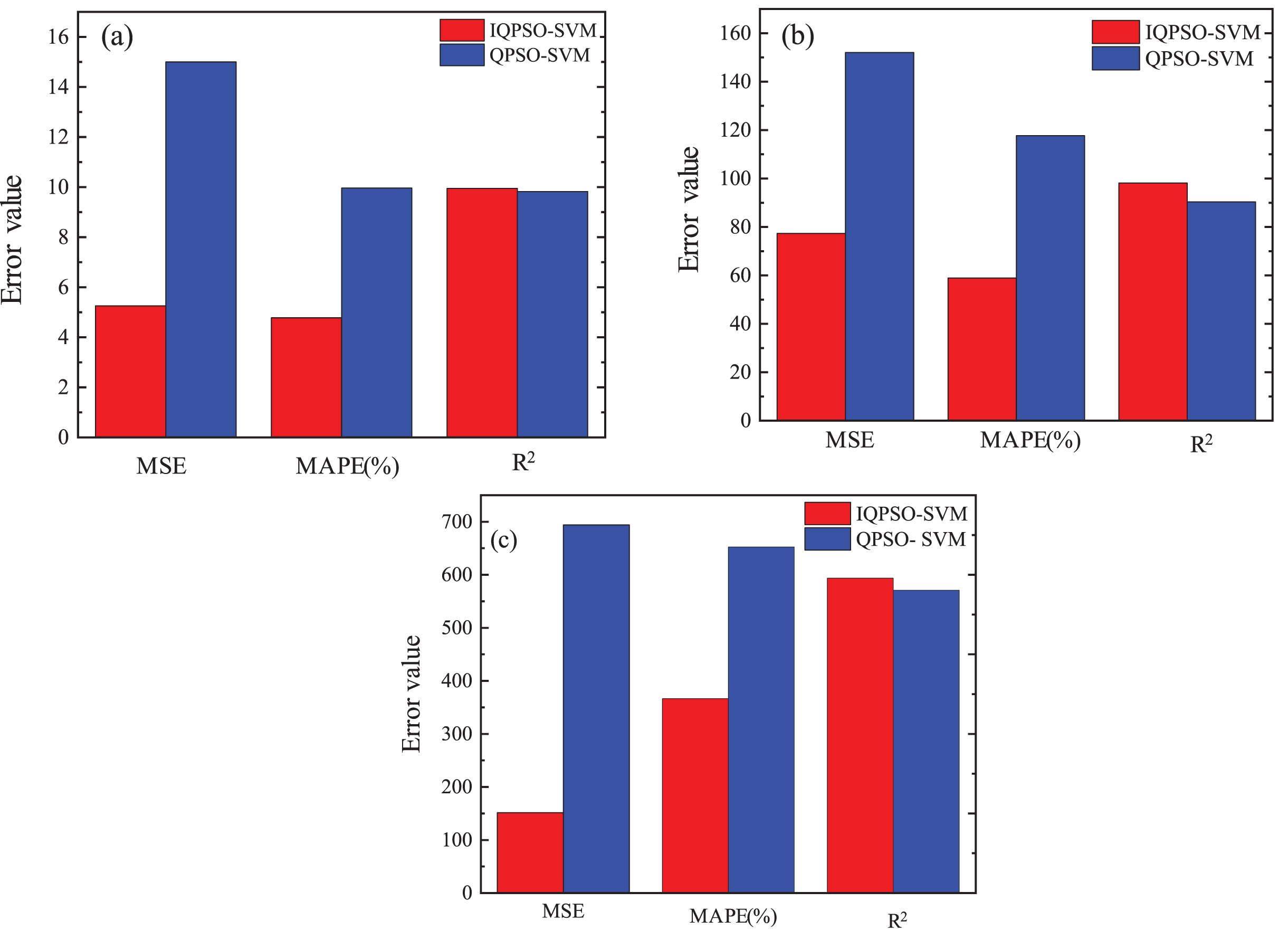
Error histograms for IQPSO-SVM and QPSO-SVM: (a) F_x; (b) F_y; and (c) F_z.

Table 9

Comparison of the evaluation indicators for IQPSO-SVM and QPSO-SVM

Predicted F /N\Index	MSE by	MSE by	MAPE by	MAPE by	R² by	R² by
	IQPSO-SVM	QPSO-SVM	IQPSO-SVM	QPSO-SVM	IQPSO-SVM	QPSO-SVM
F _x	5.2532	15.002	4.78%	9.96%	0.9949	0.9824
F _y	77.291	152.03	5.89%	11.8%	0.9814	0.9634
F _z	151.55	694.08	3.42%	6.09%	0.9894	0.9515

The comparison of the above evaluation indexes shows that the MSE of the IQPSO-SVM model is obviously smaller than that of the QPSO-SVM model, and the MAPE of the model is significantly smaller than that of the QPSO-SVM model; this finding suggests that IQPSO-SVM has higher prediction accuracy for the test set. The R² of the IQPSO-SVM model is larger than that of the QPSO-SVM model, which indicates that the fitting degree of the model is higher and that the overall data trend is better reflected by the improved model. Therefore, based on the prediction evaluation indexes, the prediction effect of the IQPSO-SVM model is obviously better than that of the QPSO-SVM model.

This paper introduces the differential evolution operator λ and improved contraction-expansion coefficient α_IQ, which accelerate the convergence speed of the algorithm and help avoid convergence to local optima and loss of generality. Additionally, the kernel function is introduced in the SVM model to linearize the complex problem, which makes the IQPSO-SVM algorithm suitable for small sample sizes and nonlinear samples, as in multidimensional milling force prediction for white marble.

6 Correlation analysis of machining parameters and the milling force

The IQPSO-SVM model can accurately predict the milling force for white marble and can determine whether this force meets the requirements of actual production in advance; additionally, the relationship between appropriate machining parameters and the milling force can be obtained. In the actual machining process, we can reverse trace the machining parameters through the predicted milling force and the correlation among the machining parameters, optimize the machining parameters, and maintain the stability of the machining process quality.

Based on the IQPSO-SVM milling force prediction model, in this section, we discuss the effect of each machining parameter on the milling force in three directions and establish a three-dimensional graph of the selected machining parameters and milling force. According to previous research, the cutting depth is positively correlated with the milling force in three directions; that is, if the depth increases, F_x, F_y, and F_z will increase. Therefore, this section does not discuss the cutting depth, and only the spindle speed n, feed speed f, milling width a_w and milling force F are considered.

6.1 Correlation analysis of machining parameters and F_x

This section establishes the relationship between the selected machining parameters and F_x, as shown in Fig. 10. Figure 10 shows that the influence of machining parameters on the milling force F_x is coupled, that is, if the feed speed and milling width are varied, the correlation between the spindle speed and F_x varies; if the spindle speed and milling width are varied, the correlation between the feed speed and F_x varies; and if the spindle speed and feed speed are varied, the correlation between milling width and F_x varies. Figure 10(a) illustrates that there is no obvious correlation among the spindle speed, feed speed and milling force F_x, which fluctuates; however, the F_x fluctuations are limited (within 15 N), so the spindle speed and feed speed have little effect on F_x. From Fig. 10(b) and Fig. 10(c), there is a clear positive linear correlation between the milling width and F_x: the larger the milling width is, the larger F_x; additionally, the smaller the spindle speed and feed speed are, the greater the influence of the milling width on F_x, that is, the larger the slope of the linear correlation.

Fig. 10

Relationship between the milling force F_x and machining parameters: (a) width of the cut is fixed at 15 mm; (b) feed speed is fixed at 5000 mm/min; (c) cutting speed is fixed at 7000 r/min.

To verify the accuracy of the above correlation analysis, some experimental data are extracted from the results in Table 2 for comparison, as shown in Table 10. Notably, when the milling width a_w increases, F_x also increases, and this finding agrees with the results of the correlation analysis.

Table 10

The correlation analysis for the milling force F_x

Number	n (r/min)	f (mm/min)	a_w (mm)	a_p (mm)	PredictedF_x (N)
4	7000	4000	12	1.5	7.109
13	7000	4000	15	1.5	11.49
19	6000	4000	12	1.5	37.69
28	6000	4000	15	1.5	52.53
44	8000	5000	12	1.5	54.17
53	8000	5000	15	1.5	92.11

6.2 Correlation analysis for machining parameters and F_y

This section establishes the relationship graph between the selected machining parameters and F_y based on the IQPSO-SVM model of white marble milling. Figure 11 shows that the influence of the machining parameters on the milling force F_y is also coupled. Notably, there is no obvious linear correlation between the spindle speed and milling force F_y. Additionally, the correlation between the spindle speed and F_y varies at different milling widths. When the cutting width is greater than or equal to 14 mm, F_y decreases first and then increases as the spindle speed increases. When the cutting width is less than 14 mm, F_y increases first and then decreases as the spindle speed increases. As shown in Fig. 11(a) and Fig. 11(b), there is an obvious positive linear correlation between the feed speed and F_y_; in other words, the higher the feed rate is, the larger F_y is. Moreover, Fig. 11(c) shows that the smaller the milling width is, the greater the effect of the feed speed on F_y. Moreover, Fig. 11(b) and Fig. 11(c) indicate that there is a significant negative linear correlation between the milling width and F_y; that is, the larger the milling width is, the smaller F_y is. Furthermore, the closer the spindle speed is to 7000 r/min, the larger the feed speed is, and the greater the effect of the milling width on F_y.

Fig. 11

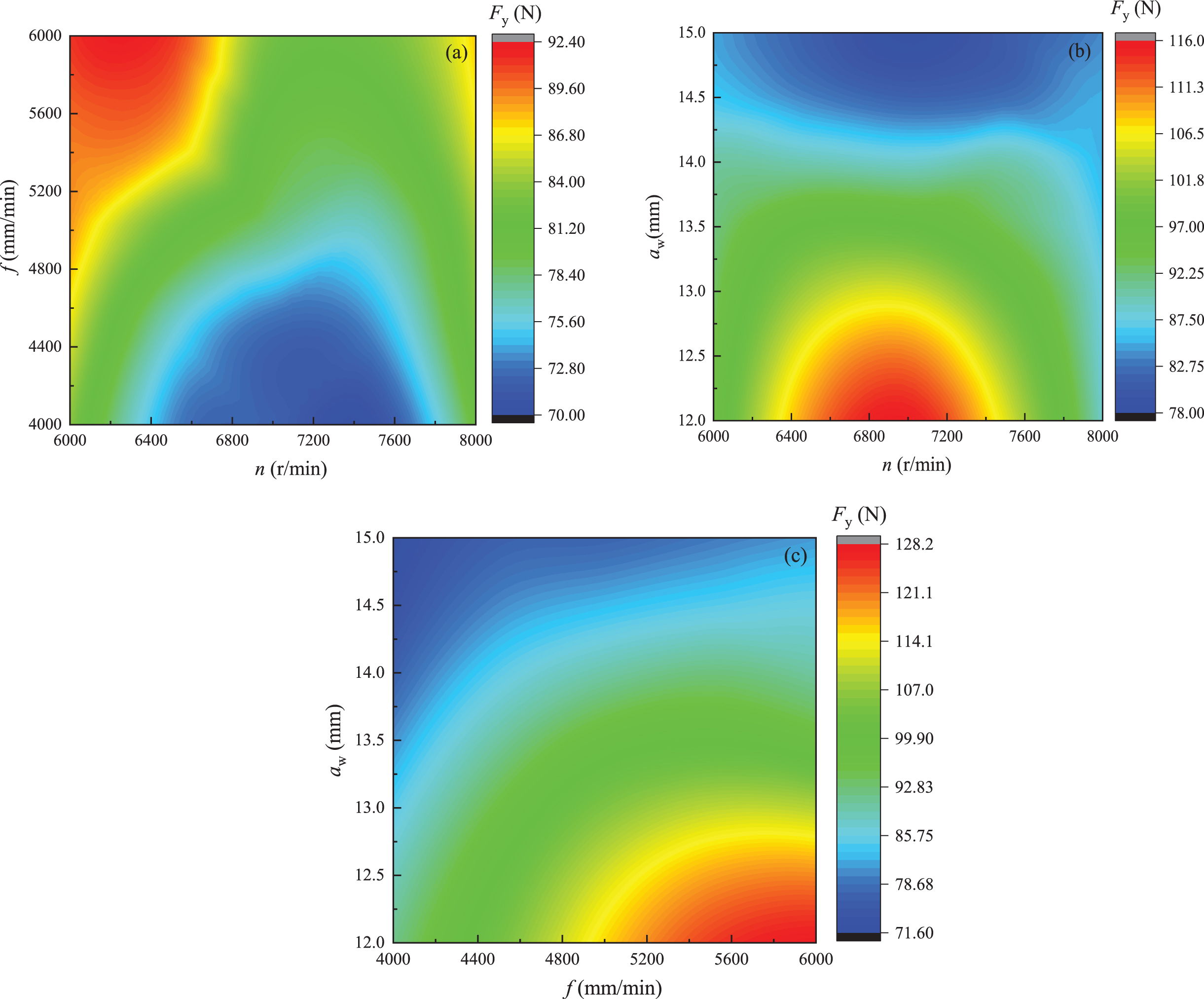
Relationship between the milling force F_y and machining parameters: (a) the cutting width is fixed at 15 mm; (b) the feed speed is fixed at 5000 mm/min; and (c) the cutting speed is fixed at 7000 r/min.

To verify the above correlation analysis, some experimental data are extracted from Table 2 for comparison, as shown in Table 11. The data for tests 20, 23, 26, 29, 32, and 35 in Table 11 show that the correlation between F_y and the spindle speed is in accordance with the analysis results. The data for 34, 35, and 36 indicate that F_y is positively related to the feed speed, and this finding supports the analysis results. From 20, 23, 26, 29, 32 and 35, we can see that F_y is negatively correlated with the milling width, and this finding supports the analysis results.

Table 11

Correlation analysis of the milling force F_y

Number	n (r/min)	f (mm/min)	a_w (mm)	a_p (mm)	PrdictedF_y (N)
20	6000	5000	12	1.5	90.42
23	7000	5000	12	1.5	120.5
26	8000	5000	12	1.5	102.4
29	6000	5000	15	1.5	85.56
32	7000	5000	15	1.5	55.56
34	8000	4000	15	1.5	46.01
35	8000	5000	15	1.5	96.95
36	8000	6000	15	1.5	117.1

6.3 Correlation analysis of the machining parameters and F_z

In this section, the relationship graph between the selected machining parameters and F_y is established based on the IQPSO-SVM model of white marble milling. From Fig. 12, there is a correlation between the machining parameters and the milling force F_z, but this correlation is smaller than those for F_x and F_y. From the graph, we can see that there is an obvious linear correlation between the milling force F_z and the spindle speed, feed speed, and milling width. Figure 12(a) and Fig. 12(b) show that there is a negative linear correlation between the spindle speed and F_z; the larger the spindle speed is, the smaller the value of F_z. Figure 12(a) and Fig. 12(c) indicate that there is a positive linear correlation between the feed speed and F_z; the larger the feed speed is, the greater the value of F_z. Figure 12(b) and Fig. 12(c) show that there is a positive linear correlation between the milling width and the F_z, and the larger the milling width is, the greater F_z is. The error in the robotic milling of machine white marble mainly comes from the deformation caused by the axial force of the cutter, that is, the deformation caused by F_z. According to the analysis results, the deformation error can be reduced by increasing the spindle speed, reducing the feed speed and reducing the milling width F_z.

Fig. 12

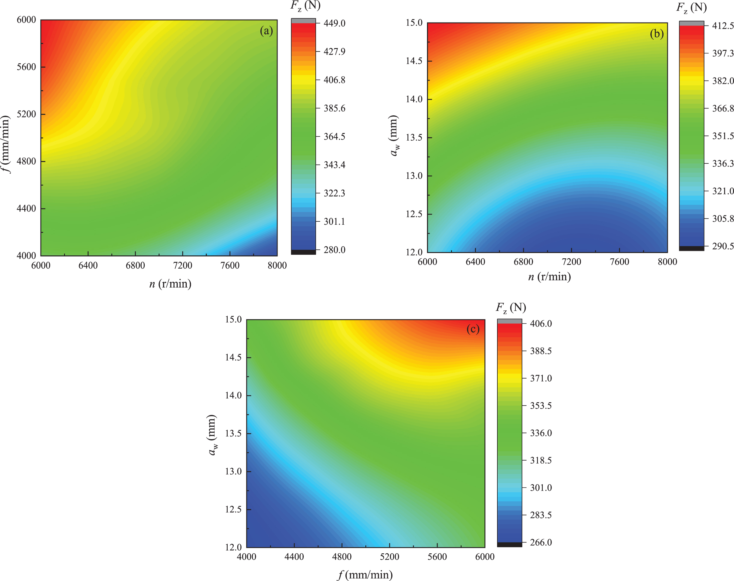
Relationship between the milling force F_z and the machining parameters: (a) the width of the cut is fixed at 15 mm; (b) the feed speed is fixed at 5000 mm/min; and (c) the cutting speed is fixed at 7000 r/min.

To verify the above correlation analysis, some experimental data were extracted from Table 2 for comparison, as shown in Table 12. From 1, 4, and 7 in Table 12, we can see that the F_z is negatively correlated with the spindle speed, and this finding supports the analysis results. From 1, 2, and 3, F_z is positively correlated with the milling width, and this result supports the analysis results. From 1, 3, 10 and 12, F_z is positively correlated with the milling width, and this finding supports the analysis results.

Table 12

The correlation analysis of the milling force F_z

Number	n (r/min)	f (mm/min)	a_w (mm)	a_p (mm)	PredictedF_z (N)
1	6000	4000	12	1.0	170.9
2	6000	5000	12	1.0	176.9
3	6000	6000	12	1.0	214.6
4	7000	4000	12	1.0	157.7
7	8000	4000	12	1.0	141.4
10	6000	4000	15	1.0	213.1
12	6000	6000	15	1.0	297.3

7 Conclusion

Considering the difficulty of white marble machining, the random fluctuations in the milling process and the complexity of the machining process, SVM regression is used to construct a prediction model of the milling force; this approach provides a certain reference value for studying the white marble machining process.

We choose the IQPSO algorithm to optimize the internal parameters of the SVM model and form the IQPSO-SVM model. A prediction model of the milling force in the white marble milling process is constructed, and the results of the proposed algorithm are compared with those of the QPSO-SVM algorithm. This paper shows the efficiency of the IQPSO-SVM model and verifies its advantages, such as requiring fewer control parameters than the QPSO algorithm, having a simple operation process and providing strong optimization ability.

Based on the verified prediction model of the milling force based on the IQPSO-SVM algorithm, the influence of machining parameters on the milling force of white marble is further explored. We construct correlation graphs between the influential parameters and target variables for the reverse tracing of the effects on the milling force. This approach provides guidance for selecting machining parameters, improving the machining process and improving the stability of the white marble milling process.

Footnotes

Acknowledgments

This work was supported by National Natural Science Foundation of China (Grant#51905181) and Natural Science Foundation of Fujian Province (Grant#2019J01084). The authors would like to thank the sponsor for this support. YFC would acknowledge the support from the “Promotion Program for Young and Middle-aged Teacher in Science and Technology Research of Huaqiao University”.

References

Wang

, Huang

S.G.

, Huang

J.X.

, et al., Parameter analysis and modelling of grinding special-shaped granite by diamond tools based on a robot stone machining system, International Journal of Abrasive Technology 10(1) (2020), 62–82.

Huang

G.Q.

, Zhang

M.Q.

, Huang

, et al., Estimation of power consumption in the circular sawing of stone based on tangential force distribution, Rock Mechanics and Rock Engineering 51 (2018), 1249–1261.

Alexander

, Anna

and Shreyes M

, Robots in machining, CIRP Annals-Manufacturing Technology 68 (2019), 799–822.

Szecsi

, Cutting force modeling using artificial neural networks, Journal of Materials Processing Technology 92-93 (1999), 344–349.

Kurt A

, Modelling of the cutting tool stresses in machining of Inconel 718 using artificial neural networks, Expert Systems with Applications 36(6) (2009), 9645–9657.

Zuperl

, A generalized neural network model of ball-end milling force system, Journal of Materials Processing Technology 175 (2006), 98–108.

Hanafi

, Cabrera

F.M.

and Khamlichi

, Artificial neural networks back propagation algorithm for cutting force components predictions, Mechanics & Industry 14(6) (2013), 431–439.

Pawade

R.S.

and Joshi

S.S.

, Multi-objective optimization of surface roughness and cutting forces in high-speed turning of Inconel 718 using taguchi grey relational analysis, International Journal of Advanced Manufacturing Technology 56(1–4) (2011), 47–62.

Ratchev

, Govender

and Nikov

, Force and deflection modelling in milling of low-rigidity complex parts, Journal of Materials Processing Technology 143-144 (2003), 796–801.

10.

Zuperl

and Cus

, Neural control strategy of constant cutting force system in end milling, Robotics and Computer-integrated Manufacturing 27(3) (2011), 485–493.

11.

Wang

Z.H.

, Liu

Y.M.

, Gong

D.Y.

, et al., A new predictive model for strip crown in hot rolling by using the hybrid AMPSO-SVR-based approach, Steel Research International 89(7) (2018), 1–12.

12.

Srivastava

, Malik

and Sharma

, A comparative simulation study of different sensorless permanent magnet synchronous motor drives using neural network and fuzzy logic, Journal of Intelligent & Fuzzy Systems 35(5) (2018), 5177–5184.

13.

L.Y.

, Lin

, Pei

H.M.

, et al., The aLS-SVM based multi-task learning classifiers, Applied Intelligence 48 (2018), 2393–2407.

14.

Benardos

P.G.

and Vosniakos

G.C.

, Predicting surface roughness in machining: A review, International Journal of Machine Tools & Manufacture 43 (2003), 833–834.

15.

Aich

and Banerjee

, Modeling of EDM responses by support vector machine regression with parameters selected by particle swarm optimization, Applied Mathematical Modelling 38(11-12) (2014), 2800–2818.

16.

Hamdi

, Ali

J.B.

and Costanzo

, Accurate prediction of continuous blood glucose based on support vector regression and differential evolution algorithm, Biocybernetics and Biomedical Engineering 38(2) (2018), 362–372.

17.

Zhang

X.L.

, Chen

X.F.

and He

Z.J.

, An ACO-based algorithm for parameter optimization of support vector machines, Expert Systems with Applications 37(9) (2010), 6618–6628.

18.

Zheng

C.H.

and Jiao

L.C.

, Automatic parameters selection for SVM based on GA. In: Proceedings of the 5th world congress on intelligent control and automation, IEEE Press, Piscataway, (2004), 1869–1872.

19.

Zhou

, Li

X.B.

, Hani

S.M.

, et al., Identification of large-scale goaf instability in underground mine using particle swarm optimization and support vector machine, International Journal of Mining Science and Technology 23(5) (2006), 740–743.

20.

Mahdi

, Mahdieh

and Hossein

, A hybrid intelligent approach to detect android botnet using smart self-adaptive learning-based PSO-SVM, Knowledge-based Systems 222(21) (2021), 106988.

21.

Ngo

T.T.

, Pham

T.D.

, Nhu

V.H.

, et al., A novel hybrid quantum-PSO and credal decision tree ensemble for tropical cyclone induced flash flood susceptibility mapping with geospatial data, Journal of Hydrology 26 (2020), 125682.

22.

Fayed

H.A.

and Atiya

A.F.

, Speed up grid-search for parameter selection of support vector machines, Applied Soft Computing 80 (2019), 202–210.

23.

Wang

X.K.

, Guan

S.Y.

, Hua

, et al., Classification of spot-welded joint strength using ultrasonic signal time-frequency features and PSO-SVM method, Ultrasonics 91 (2019), 161–169.

24.

Cervantes

, Lamont

F.G.

, Rodriguez

, et al., PSO-based method for SVM classification on skewed data sets, Neurocomputing 228(8) (2017), 187–197.

25.

Kong

and Wang

Y.M.

, Design of computer interactive system for sports training based on artificial intelligence and improved support vector, Journal of Intelligent & Fuzzy Systems 37 (2019), 6165–6175.

26.

F.L.

, Sun

Z.L.

and Zhao

, The research of automatic measuring system on stone milling force, Applied Mechanics & Materials 19 (2009), 1005–1009.

27.

Fan

X.H.

, Tian

Y.B.

and Zhao

, Optimal design of microware devices by fitness-estimation-based particle swarm optimization algorithm, Applied Computational Electromagnetics Society Journal 33(11) (2018), 1259–1267.

28.

Wan

, Zou

, Wang

K.L.

, et al., Research on hot deformation behavior of Zr-4 alloy based on PSO-BP artificial neural network, Journal of Alloys and Compounds 826(15) (2020), 154047.

29.

Shooli

A.R.

, Vosoughi

A.R.

and Banan

M.R.

, A mixed GA-PSO-based approach for performance-based design optimization of 2D reinforced concrete special moment-resisting frames, Applied Soft Computing 85 (2019), 105843.

30.

Liu

H.T.

, Zhai

R.R.

, Fu

J.X.

, et al., Optimization study of thermal-storage PV-CSP integrated system based on GA-PSO algorithm, Solar Energy 184(15) (2019), 391–409.

31.

X.Z.

, Shan

, Wang

G.Y.

, et al., Multimodal medical image fusion using PCNN optimized by the QPSO algorithm, Applied Soft Computing 46 (2016), 588–595.

32.

Chen

S.X.

, Wang

J.Q.

and Zhang

H.Y.

, A hybrid PSO-SVM model based on clustering algorithm for short-term atmospheric pollutant concentration forecasting, Technological Forecasting and Social Change 146 (2019), 41–54.

33.

Jin

, Wu

, Hu

Y.M.

, et al., Identification of thermal error in a feed system based on multi-class LS-SVM, Frontiers of Mechanical Engineering 7(1) (2012), 47–54.

An improved QPSO-SVM-based approach for predicting the milling force for white marble in robot stone machining

Abstract

Keywords

1 Introduction

2.1 Definition of the milling force of white marble

3.1 Support vector regression theory

4 Optimization of SVR with IQPSO

4.1 Basic PSO algorithm

5.1 Performance criteria

6.1 Correlation analysis of machining parameters and F x

Footnotes

Acknowledgments

References

6.1 Correlation analysis of machining parameters and F_x