A new bearing fault diagnosis method using elastic net transfer learning and LSTM

Abstract

Although the existing transfer learning method based on deep learning can realize bearing fault diagnosis under variable load working conditions, it is difficult to obtain bearing fault data and the training data of fault diagnosis model is insufficient£¬which leads to the low accuracy and generalization ability of fault diagnosis model, A fault diagnosis method based on improved elastic net transfer learning under variable load working conditions is proposed. The improved elastic net transfer learning is used to suppress the over fitting and improve the training efficiency of the model, and the long short-term memory network is introduced to train the fault diagnosis model, then a small amount of target domain data is used to fine tune the model parameters. Finally, the fault diagnosis model under variable load working conditions based on improved elastic net transfer learning is constructed. Finally, through model experiments and comparison with conventional deep learning fault diagnosis models such as long short-term memory network (LSTM), gated recurrent unit (GRU) and Bi-LSTM, it shows that the proposed method has higher accuracy and better generalization ability, which verifies the effectiveness of the method.

Keywords

Elastic net fault diagnosis LSTM transfer learning

1 Introduction

The rolling element bearing is the important part of mechanical equipment, and timely diagnosis of bearings can prevent industrial accidents [1]. However, in practical engineering applications, the bearing data is often small, and the working environment is often variable, so it is difficult to obtain the bearing fault data, which brings severe challenges to the fault diagnosis of rolling bearings [2].

Now, there are many deep learning methods used in bearing fault diagnosis [3]. Deep learning [4] overcomes the defects of traditional bearing diagnosis methods, and can automatically learn valuable features from the original data. To a large extent, it gets rid of the signal processing experience of diagnosis experts, and has been applied to bearing fault diagnosis. Nowadays, a lot of achievements have been made in fault diagnosis of rolling bearings. Amar M et al. present a novel vibration spectrum imaging (VSI) feature enhancement procedure for low SNR conditions and used ANN to classify bearing faults [5]; Wei Zhang et al. proposed a novel method named Deep Convolutional Neural Networks with Wide First-layer Kernels for bearing fault diagnosis [6]; Y Li et al. proposed a method based on multi-scale permutation entropy (MPE) and improved support vector machine based binary tree (isvm-bt), and applied it to extract vibration features of bearings [7]; Guo X et al. proposed a novel hierarchical learning rate adaptive deep convolution neural network based on an improved algorithm for bearing fault diagnosis [8]. However, these traditional methods based on deep learning have the following problems: firstly, they need to carry out complex training on the original data, secondly, they need a large number of training data to train the network, the training time is long, the manpower and material resources are expensive, and there are not a lot of training data in the actual application [9]. Aiming at the problems of traditional deep learning methods, in recent years, transfer learning is widely used in rolling bearing fault diagnosis, which has the ability to learn the knowledge and skills of previous tasks and apply them to new tasks. The transfer learning method does not need to assume the same distribution of training data and test data, and it can avoid the manpower and material costs caused by relabeling the acquired data in traditional machine learning [10]. The main idea of transfer learning is to learn knowledge from the existing source domain, and then transfer the knowledge to the target domain [11]. J Shao et al. proposed an adversarial domain adaption method based on deep transfer learning [12]; Piao Lei et al. proposes a new transferable fault diagnosis method with adaptive manifold probability distribution (AMPD) under different working conditions [13];Wang et al. proposed a transfer learning method based on ResNet [14]; Han et al. applied data enhancement to Convolutional Neural Network (CNN) and proposed a new transfer learning method [15]; Xu G et al. proposed an online fault diagnosis method based on a deep transfer convolutional neural network (TCNN) framework [16].

In this paper, the Elastic Net [17] is introduced into the bearing fault diagnosis model, and the relationship between L1 regularization and L2 regularization penalty terms is illustrated through experiments. The improved Elastic Net is added to the LSTM, and the bearing fault diagnosis is carried out by using transfer learning. The trained model parameters are transferred, and then we use a small amount of target domain data to fine-tune the network parameters, and finally realize the rolling bearing fault diagnosis under different working conditions.

2 A introduction to elastic net transfer learning

2.1 Transfer learning

The meaning of transfer learning is to apply the knowledge learned from previous tasks to new tasks [18], transfer the model parameters learned to other network models, and retrain the network. The main purpose is to improve the generalization ability of the model. Traditional machine learning requires sufficient training data to train a good model. However, for the target domain classification problems with only a small amount of data, transfer learning can be used to solve this kind of problems [19, 20]. Transfer learning can quickly train to get an ideal result, and it can also have a better effect when the data set is small [21, 22].

The two extreme forms of transfer learning are one-time learning and zero-time learning. The transfer task with only one labeled sample is called one-time learning; the transfer task without labeled sample is called zero-time learning. Only when additional information is used in training, zero-time learning is possible. There are many kinds of transfer learning methods. According to the content of transfer learning, transfer learning methods can be divided into feature-based transfer, instance-based transfer, model-based transfer, and relationship-based transfer. Table 1 shows the comparison of four different transfer learning methods.

Table 1
Comparison of different transfer learning methods

Transfer learning methods Implementation of the methods

Feature-Based Transfer Map the features of the source and target domains to the same space

Instance-Based Transfer Instantiate the source domain sample weight

Model-Based Transfer Source domain and target domain share weight parameters

Relationship-Based Transfer Find the relationship between the source domain and the target domain

Transfer learning methods	Implementation of the methods
Feature-Based Transfer	Map the features of the source and target domains to the same space
Instance-Based Transfer	Instantiate the source domain sample weight
Model-Based Transfer	Source domain and target domain share weight parameters
Relationship-Based Transfer	Find the relationship between the source domain and the target domain

2.2 Elastic net transfer learning

One of the main purposes of transfer learning is to improve the generalization ability of the model. Even if the model is applied to other test data rather than training data, the model can also have high recognition accuracy [23]. Aiming at the problem of insufficient training data of fault diagnosis model, which leads to low generalization ability of the model, this paper adopts the model-based transfer learning method to make the source domain and target domain share weight parameters, so as to improve the generalization ability of the model. In deep learning, a very key problem is how to design a model, which has a very good performance in both training data and test data. In machine learning, many methods are used to reduce test errors, suppress over fitting [24], and improve the generalization ability of models, which are called regularization [25]. At present, the commonly used regularization methods are L1 regularization and L2 regularization [26].

L1 regularization is as follows: $L_{1} = {∥ w ∥}_{1} = \sum_{i} | w_{i} |$ (1)

wrepresents the weight parameter to be updated.

L2 regularization adds the following regularization item to the objective function: $L_{2} = \frac{1}{2} {∥ w ∥}_{2}^{2} = \frac{1}{2} \sum_{i} w_{i}^{2}$ (2)

It can be seen from above formula that L2 regularization is the sum of squares of each weight parameter.

In order to further improve the generalization ability of the model, the Elastic Net is introduced in this paper.The formula is as follows: $L_{1, 2} = λ_{1} {∥ w ∥}_{1} + \frac{λ_{2}}{2} {∥ w ∥}_{2}^{2}$ (3)

λ₁ and λ₂ are penalty terms. It can be seen from the above formula that Elastic Net is a linear combination of L1 regularization and L2 regularization.

3 An improved elastic net transfer learning

Elastic Net is to add L1 regularization and L2 regularization to the loss function at the same time.The cost function after adding Elastic Net is as follows: $J (w; X, y) = L (w; X, y) + λ_{1} {∥ w ∥}_{1} + \frac{λ_{2}}{2} {∥ w ∥}_{2}^{2}$ (4)

J (w ; X, y) is the cost function, L (w ; X, y) is the loss function, λ₁ and λ₂ control the strength of regularization.

Explain the physical meaning of λ₁ and λ₂from two-dimensional space. The two-dimensional space graph of L1 regularization and L2 regularization can be expressed by the following formulas: $F_{1} = | w_{1} | + | w_{2} |$ (5) $F_{2} = w_{1}^{2} + w_{2}^{2}$ (6)

It can be seen that the two-dimensional space graph of L1 regularization is a diamond, and the two-dimensional space graph of L2 regularization is a circle. When the penalty terms λ₁ and λ₂ increase, the graph will shrink, and the corresponding weights w₁ and w₂ will also decrease; When the penalty terms λ₁ and λ₂ decrease, the graph will increase, and the weights w₁ and w₂ will also increase. Therefore, the penalty terms λ₁ and λ₂ can control the size of the weights, suppress over fitting, and improve the generalization ability of the model.

Next, in order to better adapt to the bearing fault data of rail transit, the relationship between λ₁ and λ₂ in this paper is analyzed by experiments. The experimental data is the rolling bearing data set of Case Western Reserve University, and the data sources will be introduced in Section 5. The experimental results are shown in Table 2.

Table 2

Comparison Results of The Relationship Between λ₁ and λ₂

First Group
λ ₁	0.09	0.08	0.07	0.06	0.05	0.04	0.03	0.02	0.01
λ ₂	0.1	0.2	0.3	0.4	0.5	0.6	0.7	0.8	0.9
Accuracy	0.861	0.908	0.881	0.89	0.924	0.884	0.876	0.897	0.908
Second Group
λ ₁	0.01	0.04	0.09	0.16	0.25	0.36	0.49	0.64	0.81
λ ₂	0.1	0.2	0.3	0.4	0.5	0.6	0.7	0.8	0.9
Accuracy	0.876	0.866	0.801	0.823	0.828	0.853	0.753	0.826	0.844
Third Group
λ ₁	0.067	0.129	0.188	0.242	0.293	0.34	0.384	0.426	0.464
λ ₂	0.1	0.2	0.3	0.4	0.5	0.6	0.7	0.8	0.9
Accuracy	0.879	0.876	0.839	0.813	0.803	0.832	0.857	0.846	0.862

According to the above experiments, the accuracy of the first group is higher, the accuracy of the second and third group is lower. In the second group of experiments, over fitting occurred once. And from the above three groups of experiments, it can be seen that with the value of penalty term λ₂ increase, the accuracy of the model is higher when the value of penalty term λ₁ decreases. Therefore, in order to simplify the above cost function formula, unify λ₁ and λ₂ in Elastic Net, the following improved cost function is proposed, as shown below: $J (w; X, y) = L (w; X, y) + \frac{1 - λ}{10} {∥ w ∥}_{1} + \frac{λ}{2} {∥ w ∥}_{2}^{2}$ (7)

λ is the unified penalty term. When λ takes different values, different combinations of regularization can be obtained.

When λ is equal to 0, L2 regularization will not work, only L1 regularization work on the loss function. Next, observe the performance of L1 regularization through the formula. For convenience, the penalty term of L1 regularization in the following formula is represented by λ₁, and the cost function with L1 regularization is as follows: $J (w; X, y) = L (w; X, y) + λ_{1} {∥ w ∥}_{1}$ (8)

Assuming that w^* is the optimal solution when L (w ; X, y) takes the minimum value, then the second-order Taylor expansion of L (w ; X, y) at w^* is as follows:

$L (w; X, y) = L (w^{*}; X, y) + L^{'} (w^{*}; X, y) (w - w^{*}) + \frac{L^{''} (w^{*}; X, y)}{2!} {(w - w^{*})}^{2}$ (9)

At w^*, L′ (w^* ; X, y) is equal to 0,and can be represented by Hessian matrix, so the loss function can be reduced to the following form: $L (w; X, y) = L (w^{*}; X, y) + \frac{1}{2} H {(w - w^{*})}^{2}$ (10)

The cost function is as follows: $J (w; X, y) = L (w^{*}; X, y) + \frac{1}{2} H {(w - w^{*})}^{2} + λ_{1} {∥ w ∥}_{1}$ (11)

The analytical solution of the following form can minimize this cost function: $w = sign (w^{*}) max (| w^{*} | - \frac{λ_{1}}{H}, 0)$ (12)

sign (w^*) just takes the sign of w^*. When $| w^{*} | - \frac{λ_{1}}{H} ⩽ 0$ , w is equal to 0, and L1 regularization produces a sparse solution. L1 regularization makes partial weights equal to 0, so as to improve the generalization ability of the model.

In (7), when λ is equal to 1, L1 regularization will not work, only L2 regularization work on the loss function. Next, we observe the performance of L2 regularization by studying the gradient of the cost function. In the following formula, the penalty term of L2 regularization is represented by λ₂,and the cost function with L2 regularization is as follows: $J (w; X, y) = L (w; X, y) + \frac{λ_{2}}{2} w^{T} w$ (13)

The gradient of cost function is as follows: $\frac{\partial J (w; X, y)}{\partial w} = \frac{\partial L (w; X, y)}{\partial w} + λ_{2} w$ (14)

The weight update formula is as follows: $\tilde{w} = w - α \frac{\partial J (w; X, y)}{\partial w}$ (15)

The simplified weight is as follows: $\tilde{w} = (1 - α λ_{2}) w - α \frac{\partial L (w; X, y)}{\partial w}$ (16)

α is the learning rate, $\tilde{w}$ is the updated weight; It can be seen from (16) that the weight after adding L2 regularization will be multiplied by a constant less than 1 during gradient update, and the weight will be shrunk, so as to suppress the excessive weight, obtain a simpler model with smaller parameters, and improve the generalization ability of the model.

In (7), when λ is not equal to 0 or 1, L1 regularization and L2 regularization work on the loss function at the same time, that is, Elastic Net. According to the above analysis, Elastic Net can not only generate sparse solutions, but also restrain the excessive weight, thereby further improving the generalization ability of the model.

Finally, the improved Elastic Net is added to LSTM for transfer learning, so as to realize bearing fault diagnosis.

4 Proposed Fault Diagnosis Method Based On Improved Elastic Net And Lstm

In machine learning, transfer learning is an important method used to solve the problems of difficulty in obtaining labeled data in practical applications. When we design a model and optimize it with data, we consider using independent and identically distributed training data and test data. At this time, the number of samples required is also very large, and the training optimization of the model is also takes a lot of time and resources, but transfer learning can solve the above problems. This paper uses LSTM to realize transfer learning., the structure of LSTM memory unit is shown in Fig. 1.

Fig. 1

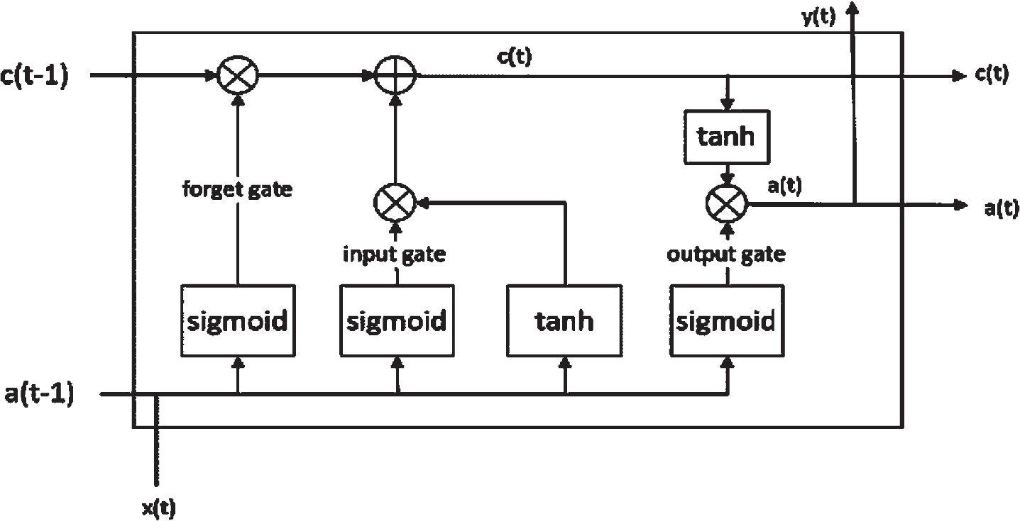
Structure of LSTM memory unit.

In this paper, we add the improved Elastic Net to LSTM to realize bearing fault diagnosis. We train the model by adding a small amount of target domain data to the source domain, and then transfer the trained model parameters to the target domain, and use a small amount of target domain data to fine tune the model parameters. Finally, we build a bearing fault diagnosis model with a certain generalization ability. Table 3 shows the fault diagnosis algorithm proposed in this paper.

Table 3

Algorithm Description Based on Elastic Net and LSTM

Algorithm 1 Fault diagnosis algorithm
Input:
Source domain data and Small amount of target domain data.
Output:
The classification results of the model after transfer learning.
Require:
z is the output of the hidden layer, z^*is the output after Batch
Norm, w is the weight parameter of the network, γ and β are
the parameters of Batch Norm to be adjusted.
Method:
The improved Elastic Net was added to the LSTM, then the
appropriate penalty term λ was selected and the model
was pre-trained.
While the model parameters did not reach the expected goals
do
for mini-batch data do
In each hidden layer,use Batch Norm to replace z with z^*.
Use back prop to compute dw,dγand dβ.
Update the parameters: w = w - αdw,
γ = γ - αdγ,
β = β - αdβ.
if the training results achieved the expected goals then
Save the model parameters and transfer them to the target
domain.
Fine-tuning parameters with a small amount of target
domain data.
Use Softmax for fault classification.
return results

Figure 2 shows the fault diagnosis process proposed in this paper based on improved Elastic Net and LSTM.

Fig. 2

The construction process of fault diagnosis model.

According to the construction process in Fig. 2, we finally built the fault diagnosis model based on improved Elastic Net transfer learning and LSTM. The method proposed in this paper can greatly reduce the complexity of parameter adjustment, and the number of penalty terms is changed from two to one, which brings great convenience to the experiment.

In the neural network, the distribution of data in each layer is constantly changing, and the change of data distribution between each layer will affect each other. The change of data distribution in the front layer will affect the back layer. Batch normalization (BN) [27] is proposed to solve the problem of data distribution changes between network layers. Therefore, BN is also added to the network model used in this paper. BN processes one mini-batch data at a time, which is to normalize the mean value and variance of the data distribution to be 0 and 1. The formulas are as follows: $μ_{B} \leftarrow \frac{1}{m} \sum_{i = 1}^{m} x_{i}$ (17) $σ_{B}^{2} \leftarrow \frac{1}{m} \sum_{i = 1}^{m} {(x_{i} - μ_{B})}^{2}$ (18) $x_{i}^{\land} \leftarrow \frac{x_{i} - μ_{B}}{\sqrt{σ_{B}^{2} + ɛ}}$ (19)

B is the set of m input data of a mini-batch, B ={ x₁, x₂, . . . , x_m }, μ_B is mean value, $σ_{B}^{2}$ is the variance, ɛ is a minimum in order to prevent the possibility of dividing by 0. Then, BN will translate and scale the normalized data [28], the formula is as follows: $y_{i} = γ x_{i}^{\land} + β$ (20)

γ and β are parameters, the initial value of γ is 1, and the initial value of β is 0, which can be adjusted to the value suitable for the network model through learning.

The above is the batch normalization algorithm. The purpose of adding BN is not to make the data distribution fluctuate too much with the increase of the number of network layers, which means that no matter how the input value changes, it can ensure that their mean value is 0 and the variance is 1, or they depend on γ and β.

5 Model validation experiment

5.1 Introduction of data sources

In this paper, the rolling bearing data set of Case Western Reserve University is used for fault identification experiment. The experimental platform is mainly composed of a 1.5KW motor, a torque sensor / decoder, a power tester and electronic controller. The processed faulty bearing was reassembled into the test motor, and the data of vibration acceleration signal under the motor load conditions of 0HP, 1HP, 2HP and 3HP was record respectively. The rolling bearing fault data set used in this paper is generated at the driving end of 12 kHz, the faults are located in the outer ring, inner ring and rolling elements, and the diameters of the faults are 0.1778 mm, 0.3556 mm and 0.5334 mm. The source domain data is 1HP and the target domain data is 2HP.

5.2 Comparison experiments of model before and after adding Elastic Net

The method proposed in this paper is compared with the conventional LSTM. The experimental results are shown in Fig. 3 and Fig. 4.

Fig. 3

The conventional LSTM model.

Fig. 4

The method proposed in this paper.

It can be seen from Fig. 3 and Fig. 4 that the difference between the recognition accuracy of training data and the recognition accuracy of test data is shrunk compared with the model without Elastic Net. However, it should be noted that the training accuracy of the model with improved Elastic Net is reduced, which does not affect the accuracy of the test data. By increasing the number of training, the training accuracy can reach 100%. Moreover, by increasing the number of training, the accuracy of the model with Elastic Net is higher than that of the model without Elastic Net. The above experiments show that the over fitting is restrained and the generalization ability of the model is improved.

5.3 Comparison experiments of different models

In order to further demonstrate the feasibility of the method proposed in this paper, we visualize the experimental results. The experimental results are shown in Fig. 5 and Fig. 6.

Fig. 5

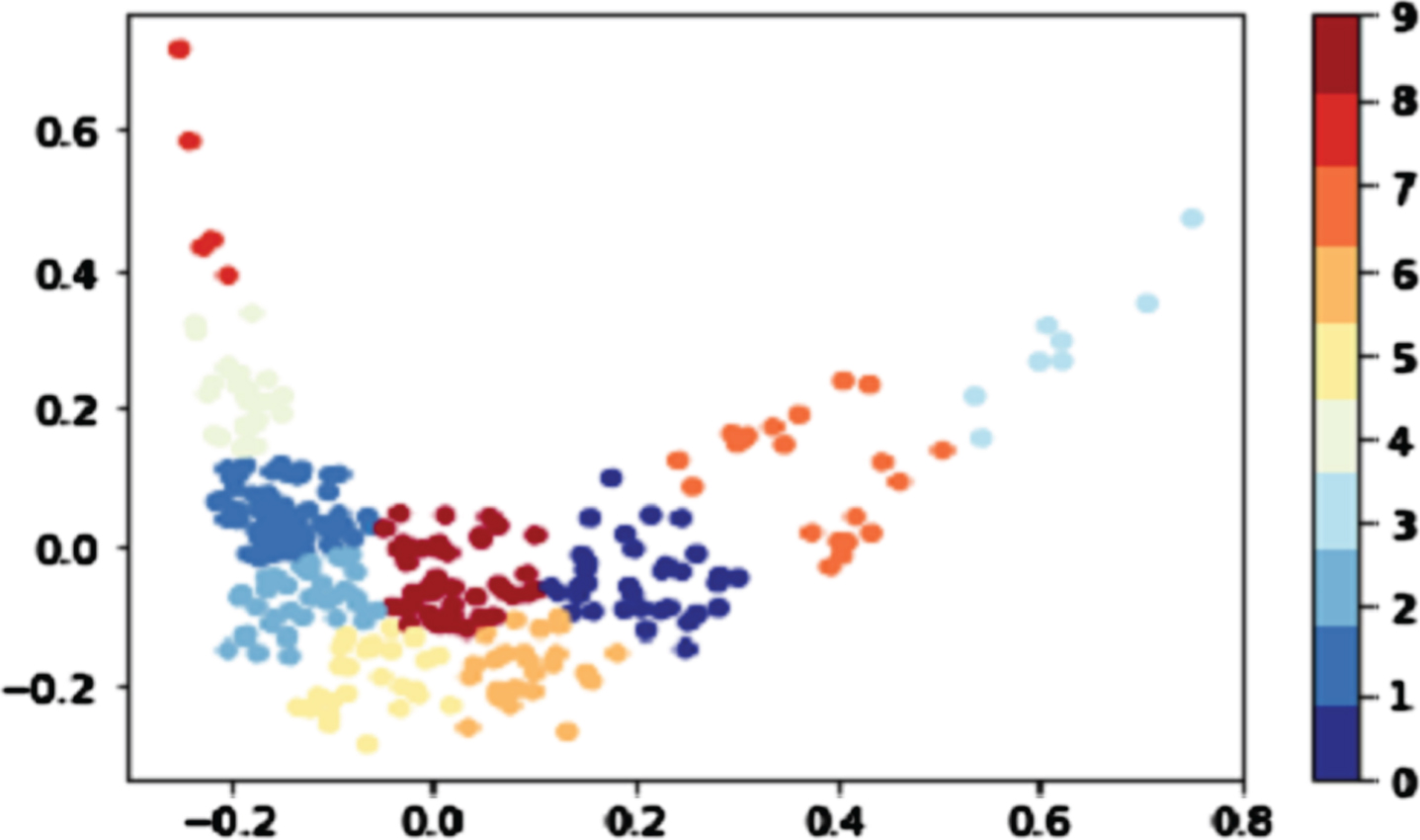
The conventional LSTM model.

Fig. 6

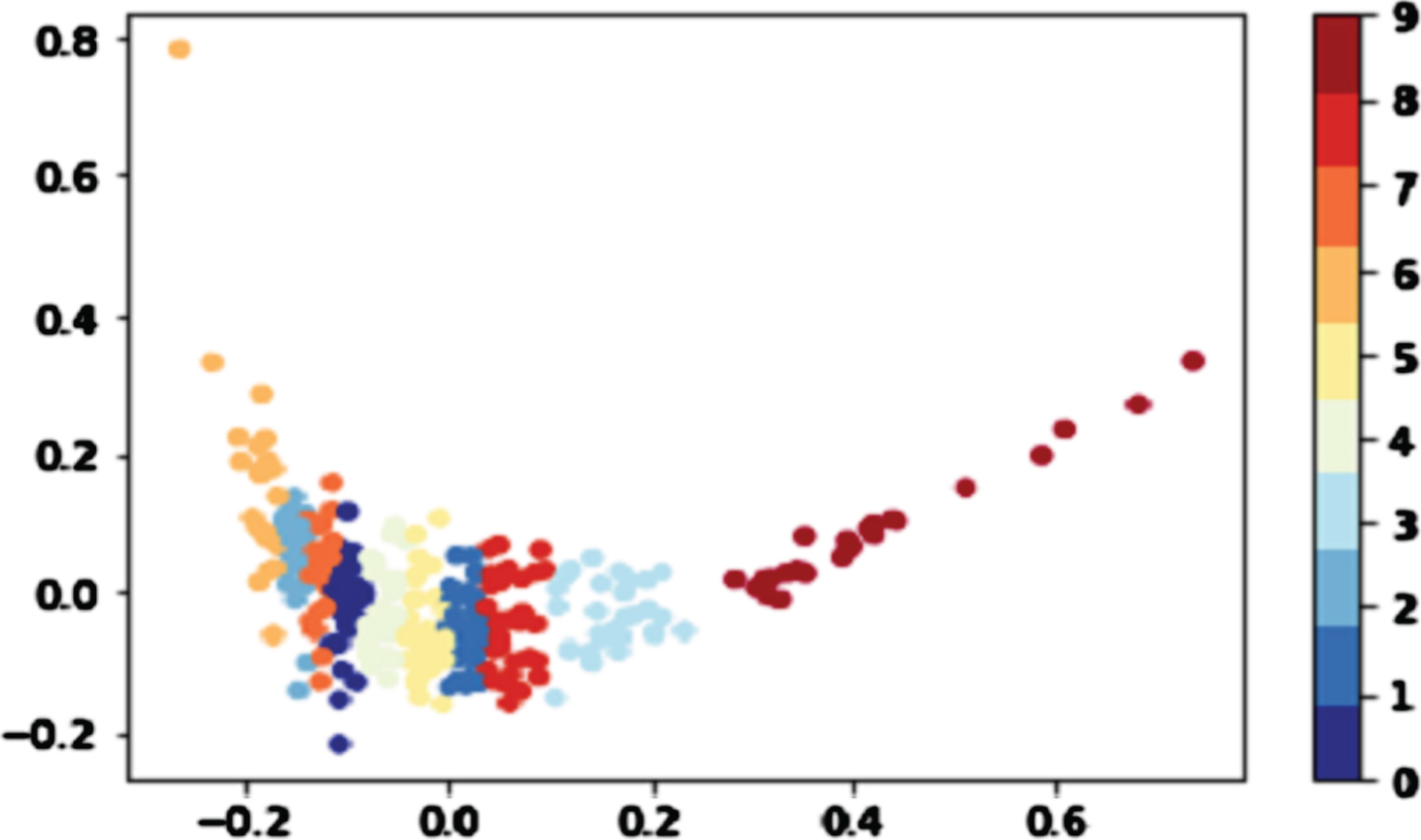
The method proposed in this paper.

As can be seen from Fig. 5 and Fig. 6, the method proposed in this paper is better.

In this paper, the LSTM with improved Elastic Net was compared with traditional LSTM, GRU and Bi-LSTM. Table 4 shows the comparison results.

Table 4

Comparison results of different network models

Network Models	Accuracy	Loss Rate
LSTM	93.8	0.377
GRU	89.3	0.546
Bi-LSTM	87.8	0.424
Elastic Net	96.3	0.298

For LSTM with Elastic Net, the generalization ability of the model is improved and the over fitting is restrained, which can improve the accuracy of the model. However, the generalization ability of the other three models is not high and over fitting is easy to occur. Under variable load conditions, the difference between the recognition accuracy of training data and test data will be enlarged, so the accuracy is not as high as the method proposed in this paper.

In order to further verify the effectiveness of the method proposed in this paper, the LSTM with Elastic Net is compared with other methods, and the comparison results are shown in Table 5.

Table 5

Comparison results of different methods

Method	Accuracy
Reference [28]	95.83
Reference [29]	92.9
Elastic Net	96.3

It can be seen from Table 5 that the method proposed in this paper is higher than that in reference [29] and reference [30], which further proves the effectiveness of the method proposed in this paper.

5.4 Comparative experiments under different training times

The proposed method in this paper and the conventional LSTM, GRU and Bi-LSTM were trained under 1HP, and then transferred to 2HP. The accuracy of the four methods was compared under different training times. The experimental results are shown in Fig. 7.

Fig. 7

Comparison results of different training times.

As can be seen from Fig. 7, with the increase of training times, the accuracy of the models is on the rise. The accuracy of the proposed method under different training times is higher than that of the other three transfer learning models.

5.5 Comparative experiments under different test samples

Experiments were carried out under different number of target domain samples, and the LSTM with improved Elastic Net was compared with the traditional LSTM, GRU and Bi-LSTM to observe the accuracy. The comparison results are shown in Fig. 8.

Fig. 8

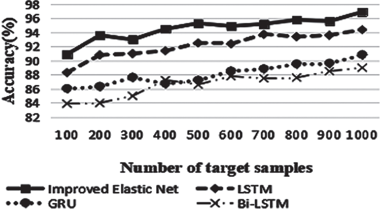
Comparative experiments under different number of target samples.

The Fig. 8 shows that the performance of the model proposed in this paper is much better than the other three models, further verify the feasibility of the proposed method in this paper.

6 Conclusion

In this paper, aiming at the problems of less rolling bearing data and difficulty in obtaining bearing fault data in practical application scenarios, a fault diagnosis method based on Elastic Net transfer learning and LSTM is proposed. This method can suppress over-fitting and improve the generalization ability of the model. The LSTM with improved Elastic Net is compared with the conventional LSTM, GRU and Bi-LSTM through related experiments to further verify the effectiveness and feasibility of the method proposed in this article.

In future work, we can judge the similarity between the source domain samples and the target domain samples, and avoid negative transfer, so as to further improve the accuracy of bearing fault diagnosis.

Footnotes

Acknowledgments

This work has been supported by Liaoning Provincial Natural Science Foundation of China (No. 2019-ZD-0105).

References

Zou

, Hou

, Lei

, et al., Bearing Fault Diagnosis Method Based on EEMD and LSTM, International Journal of Computers, Communications & Control 15(1), 2020.

Qiao

, Yan

, Tang

, et al., Deep Convolutional and LSTM Recurrent Neural Networks for Rolling Bearing Fault Diagnosis Under Strong Noises and Variable Loads, IEEE Access 99 (2020), 1–1.

Pan

H.H.

, et al., An Improved Bearing Fault Diagnosis Method using One-Dimensional CNN and LSTM, Journal of Mechanical Engineering, 2018.

Schmidhuber

, Deep learning in neural networks:An overview, Neural Networks 61(1) (2015), 85–97.

Amar

, Gondal

and Wilson

, Vibration Spectrum Imaging: A Novel Bearing Fault Classification Approach, IEEE Transactions on Industrial Electronics 62(1) (2015), 494–502.

Wei

, Gaoliang

, Chuanhao

, et al., A New Deep Learning Model for Fault Diagnosis with Good Anti-Noise and Domain Adaptation Ability on Raw Vibration Signals, Sensors 17(2) (2017), 425.

, Xu

, Wei

, et al., A new rolling bearing fault diagnosis method based on multiscale permutation entropy and improved support vector machine based binary tree, Measurement 77 (2016), 80–94.

Guo

, Chen

and Shen

, Hierarchical adaptive deep convolution neural network and its application to bearing fault diagnosis, Measurement 93 (2016), 490–502.

Wang

, Liu

, Chen

, et al., A deformable CNN-DLSTM based transfer learning method for fault diagnosis of rolling bearing under multiple working conditions, International Journal of Production Research (2020), 1–15.

10.

, Jiang

, Zhao

, et al., An adaptive deep transfer learning method for bearing fault diagnosis, Measurement 151 (2019), 107227.

11.

, Yu

, Han

, et al., A Generic Intelligent Bearing Fault Diagnosis System Using Convolutional Neural Networks With Transfer Learning, IEEE Access 8 (2020), 164807–164814.

12.

Shao

, Huang

and Zhu

, Transfer Learning Method Based on Adversarial Domain Adaption for Bearing Fault Diagnosis, IEEE Access 99 (2020), 1–1.

13.

, CS

, BD

, et al., A new transferable bearing fault diagnosis method with adaptive manifold probability distribution under different working conditions – Science Direct, Measurement, 2020.

14.

Wang

, Xie

and Zhang

, Deep learning for bearing fault diagnosis under different working loads and non-fault location point, Journal of Low Frequency Noise Vibration and Active Control (2019), 1–13.

15.

Dongmei

, Qigang

and Weiguo

, A new image classification method using CNN transfer learning and web data augmentation, Expert Systems with Application 4174(17) (2018), 43–56.

16.

, Liu

, Jiang

, et al., Online Fault Diagnosis Method Based on Transfer Convolutional Neural Networks, IEEE Transactions on Instrumentation and Measurement 99 (2019), 1–12.

17.

Shengyue

, Changkun

and Liuyan

, Flood Forecast Based on Regularized GRU Model, Computer Systems & Applications 28(5) (2019), 196–201.

18.

O’Neill

and Bollegala

, Dropping networks for transfer learning. 2018,arXiv:1804.08501.[Online]. Available: http://arxiv.org/abs/1804.08501.

19.

Yan

, Shen

, Sun

, et al., Knowledge transfer for rotary machine fault diagnosis, IEEE Sensors Journal 20(15) (2020), 8374–8393.

20.

Wen

, Gao

and Li

, A new deep transfer learning based on sparse auto-encoder for fault diagnosis, IEEE Trans Syst, Man, Cybern, Syst 49(1) (2019), 136–144.

21.

Zhang

, Tao

, Wu

, et al., Transfer learning with neural networks for bearing fault diagnosis in changing working conditions, IEEE Access 5 (2017), 14347–14357.

22.

Cao

, Zhang

and Tang

, Preprocessing-free gear fault diagnosis using small datasets with deep convolutional neural network-based transfer learning, IEEE Access 6 (2018), 26241–26253.

23.

Shao

, McAleer

, Yan

, et al., Highly accurate machine fault diagnosis using deep transfer learning, IEEE Trans Ind Informat 15(4) (2019), 2446–2455.

24.

Jian

, Lei

, Qianqian

, et al., Research on Pedestrian Gait Recognition Based on Multi-scale Feature Transfer Learning, Computer Engineering and Applications (2020), 1–13.

25.

Lijie

, Shida

, Shuo

, et al., Ball Mill Load Condition Recognition Model Based on Regularized Stochastic Configuration Networks, Control Engineering of China 27(1) (2020), 1–7.

26.

Shufen

, Chen

, Chuanbo

, et al., The CNN-L1/L2-ELM Hybrid Architecture Used to Classify Pulmonary Nodules, Journal of WUYI University 34(2) (2020), 46–53.

27.

Lichao

, Yaodong

, Rui

, et al., Welding defect classification of stainless steel based on AlexNet neural network combined with transfer learning, CAAI Transactions on Intelligent Systems (2020), 1–7.

28.

Junjie

, Xianyong

, Zengbing

, et al., Bearing fault diagnosis based on unsupervised transfer component analysis and deep belief network, Journal of Wuhan University of Science and Technology 42(06) (2019), 456–462.

29.

Mingwu

, Research on Fault Diagnosis Method of Rolling Bearings under Variable Working Conditions based on Transfer Learning, Harbin University of Science and Technology, 2019.