A novel grey model of impulse delay and its application in forecasting stock price

Abstract

The stock market is an important embodiment of a national economy and financial activities and has an important impact on a country, enterprises and individuals. Stock forecasting can allow investment institutions and investors to understand the trend of the stock market in advance, which is a challenging and meaningful study. First, through the impulse phenomenon of the stock market, this paper discusses the problem of stock price prediction with delay, and the impulse delay differential equation is established. Second, according to the difference between the differential and the difference, the nonlinear delay grey prediction model is established. Next, the model parameters are estimated and the solving steps are obtained. The nonlinear parameters and delay time are optimized by the particle swarm optimization algorithm. Finally, the new model is applied to the prediction of the Shanghai stock market and the Shenzhen stock market closing indexes; the results show that the new model can effectively predict stock prices, which is much better than the existing four grey models and a time series model.

Keywords

Stock price impulse delay grey model forecasting

1 Introduction

Finance is the core of the modern market economy and plays an increasingly important role in China’s economic reform and development. The stock market is an important embodiment of the national economy and financial activities, plays a significant role in China’s economic development, and has an important impact on the country, enterprises and individuals. If someone can understand the trend of the stock market in advance, this will bring benefits to investment institutions and investors. Using scientific and effective technology to analyse indicators and stock price change trends of the future, more accurate predictions can be made. This can provide investors with predictions of stock price movements in the future and specify a reasonable investment strategy to make good profits into the future. Therefore, the prediction of the trend of stock price changes in the stock market can provide the majority of investors a further understanding of the stock market. This not only has profound theoretical significance but also has more important practical significance to conduct in-depth research on the testability of the stock market.

Stock forecasting is a branch of economic projection that mainly uses scientific methods to uncover effective information from the historical data of stock prices, clarifies the change rules and makes accurate predictions. The prediction techniques of stock prices can be roughly divided into the following three methods: traditional time series forecasting, machine learning forecasting and combination forecasting [1]. The time series forecasting method is mainly based on a large number of discrete stock prices to explore the law of stock price changes with time to perform modelling. Paola et al. [2] applied the vector error correction model to the high-frequency time series of a foreign exchange market and predicted high-frequency data in the financial field. The numerical experiment showed that the results were better than the effect of the autoregressive integrated moving average (ARIMA) model and other models. Machine learning methods mainly include neural network models and random forests. For example, Ajit et al. [3] proposed a low-complexity recursive neural network model for stock price prediction and its prediction performance showed that the effect was better than other neural network models. Hyeuk et al. [4] used the improved random forest bootup method to predict stock index prices; the results were better than those of other machine learning methods. The combination prediction method combines various algorithms for prediction modelling. For example, Jigar et al. [5] used a multifusion machine learning method to forecast stock market indexes, which has a better effect than a single neural network and other methods. Paiva [6] combined the support vector machine method and the mean method into a model to predict stock returns by the daily investment value.

Most of the above forecasting models require considerable historical data, their calculations are complex, and most of them assume that stock prices change in a linear fashion. However, due to the complex nonlinear relationship between stock prices and influencing factors, which is stochastic and mutable, it is difficult to describe with an accurate mathematical model. Therefore, its prediction accuracy is low and it lacks practicality [7]. The stock price is a comprehensive result of multiple factors, the influencing factors are grey and uncertain, and the grey prediction model is characterized by a simple calculation. Therefore, many scholars regard the stock price system as a grey system and make predictions on it with relatively high prediction accuracy.

Grey system theory has been widely considered since it was proposed in 1982 [8]. The grey prediction model is one of the core contents of grey system theory, which is characterized by simple calculation; it is superior to traditional prediction methods. It has been widely used in short-term traffic flow prediction [9], traffic safety prediction [10], energy consumption prediction [11 –15], economic management [16] and other fields. However, traditional grey prediction univariate models, such as the GM(1,1) model, DGM(1,1) model [17, 18], multivariable grey GM(1,N) model, and NGM (1,N) model [19, 20], also have many defects. Therefore, to improve the simulation and prediction performance of the grey prediction model, researchers have extended the existing classic grey univariate and multivariate models to the new grey prediction model [21 –23]. Concurrently, a large number of in-depth and systematic studies were performed on the grey prediction model from the perspectives of the modelling mechanism, model properties and model combination, which promoted the development and improvement of the theoretical system of the grey prediction model [24 –26].

There are also many papers on the application of the grey prediction model in stock price prediction, such as the GM(1,1) and Verhulst models improved by the Fourier series by Kayacan et al. [27], which are mainly used to study the short-term prediction of stocks. Duan et al. [28] used the nature of the Fibonacci sequence to optimize the background value of the GM(1,1) model and used the inflexion point data of Elliott’s wavy line as the original modelling data to make short-, medium- and long-term predictions on stocks. Wu et al. [29] used the grey GM(1,1) model to predict stock prices, which had certain effects. Wang et al. [30] applied grey system theory to the stock market and predicted the stock price index, which proved that it was feasible and reasonable.

The applications above basically applied the grey prediction model according to the time series of the stock price. However, there is an impulse phenomenon in the stock market [31] and its mathematical model can often be summed up as an impulse differential system. When the pulse phenomenon occurs, the state variable of the system can change considerably in a very short time and the stock prices are delayed [32]. This delay refers to the system input and output not matching at a specific time, i.e., there is a time lag between the system input and output. The grey forecasting models above did not consider the stock delay phenomenon, so they cannot reach the expected effect for stock prediction. The research motive of this paper is that the stock price system is an impulse system with a delay phenomenon. Based on this phenomenon, a new grey prediction model is studied and applied to stock price prediction.

Based on the impulse phenomenon of the stock market, this paper studied the differential equation of the impulse delay. According to the difference in the grey system between the differential and the difference, the corresponding nonlinear grey prediction model of the delay is established, the model parameters are estimated and the solving steps are obtained. Additionally, the model is applied to the Chinese stock market to predict the stock prices in the Shanghai and Shenzhen Stock Indexes of two typical stocks, Kweichow Moutai and AIER Eye Hospital. The results show that the effect of the model is better than that of the four other grey prediction models and the non-grey ARIMA model that were compared. This model can effectively predict the price of stocks on the Chinese stock market. Therefore, the main contributions of this paper are as follows:

We introduced the impulse phenomenon of the stock market to the grey prediction model, established the delayed grey prediction model and studied the properties of the model.

We established a nonlinear grey prediction model with the complex nonlinear relationship between the stock price and the influencing factors. Then, we used the particle swarm optimization algorithm (PSO) to optimize the delay time and nonlinear items.

Taking the Shanghai Stock Index, Shenzhen Stock Index and two important stocks as examples, we verified the effect of the model. The results show that the new model can effectively predict Chinese stock prices.

In the full text, we use different abbreviations for different grey prediction models. These abbreviations and their meanings are listed in Table 1.

Table 1
Abbreviations of models

Number Abbreviation Definition

1. ARIMA Autoregressive integrated moving average model [33]

2. Verhulst Grey Verhulst model [34]

3. DGM(1,1) Discrete grey model with one variable and one first-order equation [35]

4. NGBM(1,1) Nonlinear grey Bernoulli model [36]

5. WGM(1,1) Grey prediction model of wave sequence based on a smoothing operator [37]

6. DSPGM(1,1| τ ,r) Grey forecasting model of stock price delay

Number	Abbreviation	Definition
1.	ARIMA	Autoregressive integrated moving average model [33]
2.	Verhulst	Grey Verhulst model [34]
3.	DGM(1,1)	Discrete grey model with one variable and one first-order equation [35]
4.	NGBM(1,1)	Nonlinear grey Bernoulli model [36]
5.	WGM(1,1)	Grey prediction model of wave sequence based on a smoothing operator [37]
6.	DSPGM(1,1\| τ ,r)	Grey forecasting model of stock price delay

The remainder of this paper is organized as follows: Section 2 establishes the differential equation under the impulse state; Section 3 establishes the grey prediction model with nonlinear delay and obtains the modelling steps of the model; Section 4 optimizes the delay time and nonlinear terms by using the PSO algorithm; Section 5 applies the model to the prediction of Chinese stock prices; and the conclusion is shown in Section 6.

2 Impulse delay differential equation

In this section, the impulse delay differential equation is established mainly through the impulse phenomenon of price [31].

Assuming that the trend function of technical traders at time t is Q_c (t), u (t) represents the future market price and the following is true [31]: $\begin{matrix} Q_{c} (t) = tanh (β_{c} (P (t) - u (t))) \end{matrix}$ where β_c represents the extrapolation rate of the trend trader to the price. The weight ρ is introduced between the market price and the basic price and the current price P (t) is represented by ρP (t) + (1 - ρ) F (t), whereρ ∈ [0, 1],P (t) is defined as follows: $\begin{matrix} \frac{dP (t)}{dx} = μ [α Q_{f} (t) + (1 - α) Q_{c} (t)] \end{matrix}$ where μ > 0 is the speed at which market makers adjust market prices. Q_f (t) is the demand function of the basic traders at time t and the demand function is proportional to the deviation between the market price and the base price, i.e., Q_f (t) = β_f (F (t) - p (t)). $\begin{matrix} \frac{du (t)}{dx} = & \frac{k}{1 - e^{- k τ_{1}}} [p (t) - e^{- k τ_{1}} p (t - τ_{1}) \\ + 1 - e^{- k τ_{1}}) u (t)] \end{matrix}$

Considering that the base price is closely related to market demand, the base price will be adjusted depending on market demand. The basic price function is given as follows:

$\begin{matrix} \frac{dF (t)}{dx} = δ [β_{f} (F (t) - p (t) + β_{c} (p (t) - p (t - τ_{2})))] \end{matrix}$

where δ represents the rate at which the base price adjusts relative to market demand.

Based on the above analysis, financial stock prices are expressed as the following system with delayed differential Equations (1), (2) and (3):

$\frac{dp (t)}{dx} = μ [\begin{matrix} α β_{f} (F (t) - p (t)) + (1 - α) tanh (β_{f} (F (t) - p (t))) \\ + (1 - α) tanh (β_{c} (ρ p (t) + (1 - p) tanh (β_{c} (ρ p (t) + (1 - ρ) F (t) - u (t))))) \end{matrix}]$ (1)

$\begin{matrix} \frac{du (t)}{dx} = \frac{k}{1 - e^{- k τ_{1}}} \\ [p (t) - e^{- k τ} p (t - τ_{1}) + (1 - e^{- k τ_{1}}) u (t)] \end{matrix}$ (2)

$\frac{dF (t)}{dx} = δ [β_{f} (F (t) - p (t) + β_{c} (p (t) - p (t - τ_{2})))]$ (3)

Obviously, p (t) = u (t) = F (t) is the equilibrium point of the system, so we call (p, u, F) = (F, F, F) the basic stable state of the system and the price at the stable state is given by a constant. We assume that the price at the stable state is $\bar{F}$ and the basic stable state of the system can be approximated as $(p, u, F) = (\bar{F}, \bar{F}, \bar{F})$ .

Now, consider the equilibrium point $(p, u, F) = (\bar{F}, \bar{F}, \bar{F})$ , let $x_{1} = p - \bar{F}, x_{2} = u - \bar{F}$ , and $x_{3} = F - \bar{F}$ , and after adding impulse control, Equations (1) through (3) can be changed into the following equation:

$\frac{dX}{dx} = AX + GX (t - τ_{i}) + f (t, X), t = t_{k}$ (4) where f (t, X) is a nonlinear term. In Equation (4), let X = p (t) be the stock price. Then, obtain the following equation:

$\frac{{dp}^{(1)} (t)}{dx} = {ap}^{(1)} (t) + {bp}^{(1)} (t - τ) + f (t, p^{(1)} (t))$ (5)

3 Grey forecasting model of stock price with time delay

This section determines the nonlinear term of differential Equation (5) according to the grey difference information, namely, the differential and the relationship between the difference, to establish the grey forecasting model of nonlinear stock price impulse time delay (denoted as the DSPGM(1,1|τ,r) model), then work to estimate the parameters and the model solution.

3.1 Establishment of model

Let the original sequence of stock prices be the following:

$X^{(0)} = (x^{(0)} (1), x^{(0)} (2), \dots, x^{(0)} (n))$ (6)

The first-order accumulating generation sequence is defined as follows:

$X^{(1)} = (x^{(1)} (1), x^{(1)} (2), \dots, x^{(1)} (n))$ (7) where $x^{(1)} (k) = \sum_{i = 1}^{k} x^{(0)} (i), k = 1, 2, \dots, n .$ .

Z⁽¹⁾ is adjacent to the mean generation sequence of X⁽¹⁾, as follows:

$Z^{(1)} = {z^{(1)} (2), z^{(1)} (3), \dots, z^{(1)} (n)}$ (8) where $z^{(1)} (k) = \frac{1}{2} (x^{(1)} (k) + x^{(1)} (k - 1))$ .

Let the nonlinear term of Equation (5) be f (t, p⁽¹⁾ (t)) = uk^r, where r is an arbitrary constant. The determination of the nonlinear term is mainly to adjust the balance state of the price system. The following whitening equation can be obtained:

$\frac{{dx}^{(1)} (t)}{dt} = {ax}^{(1)} (t) + {bx}^{(1)} (t - τ) + {ut}^{r}$ (9)

Then, the grey prediction model below can be defined.

Definition 1. The sequences X⁽⁰⁾, X⁽¹⁾ and Z⁽¹⁾ are as shown in Equations (6), (7) and (8); then, the grey forecasting model of stock price delay is given as follows:

$x^{(0)} (k) = {az}^{(1)} (k) + {bz}^{(1)} (k - τ) + {uk}^{r}$ (10) where τ represents the delay time, r represents the adjustment of the nonlinear term frequency, and k = τ + 2, τ + 3, . . . , n. This model is referred to as a grey model of stock price with time delay (denoted as the DSPGM(1,1|τ,r) model), and Equation (9) is the whitening equation of this model.

3.2 Estimation of parameters and model solution

The parameter estimation formula of the model can be obtained from Definition 1. It is given by the following theorem:

Theorem 1. Parameters of the DSPGM(1,1|τ,r) model are [a, b, u] ^T = (B^TB) ^-1BY , where the following is true: $\begin{matrix} Y = [\begin{matrix} x^{(0)} (τ + 2) \\ x^{(0)} (τ + 3) \\ \dots \\ x^{(0)} (n) \end{matrix}] \end{matrix}$ $\begin{matrix} B = [\begin{matrix} \frac{1}{2} (x^{(1)} (τ + 2) + x^{(1)} (τ + 1)) \frac{1}{2} (x^{(1)} (2) + x^{(1)} (1)) \dots (τ + 2)^{r} \\ \frac{1}{2} (x^{(1)} (τ + 3) + x^{(1)} (τ + 2)) \frac{1}{2} (x^{(1)} (3) + x^{(1)} (2)) \dots (τ + 3)^{r} \\ ⋮ ⋮ ⋱ ⋮ \\ \frac{1}{2} (x^{(1)} (n) + x^{(1)} (n - 1)) \frac{1}{2} (x^{(1)} (n - τ) + x^{(1)} (n - τ - 1)) \dots n^{r} \end{matrix}] \end{matrix}$

Proof. Substituting x⁽¹⁾ (k) - x⁽¹⁾ (k - 1) = x⁽⁰⁾ (k) into the whitening differential equation $\frac{{dx}^{(1)} (t)}{dx} = {ax}^{(1)} (t) + {bx}^{(1)} (t - τ) + {ut}^{r}$ to replace the derivative $\frac{{dx}^{(1)} (t)}{dx}$ gives the following: $\begin{matrix} x^{(0)} (k) = {ax}^{(1)} (k) + {bx}^{(1)} (k - τ) \\ + {uk}^{r}, k = τ + 2, τ + 3, \dots, n \end{matrix}$

Then, replacing x⁽¹⁾ (k) and x⁽¹⁾ (k - τ) with $z^{(1)} (k) = \frac{1}{2} (z^{(1)} (k) + z^{(1)} (k - 1))$ and z⁽¹⁾ (k - τ) = $\frac{1}{2} (z^{(1)} (k - τ) + z^{(1)} (k - τ - 1))$ gives the following equation system: $\begin{matrix} {\begin{matrix} x^{(0)} (τ + 2) = \frac{1}{2} (x^{(1)} (τ + 2) + x^{(1)} (τ + 1)) \cdot a + \frac{1}{2} (x^{(1)} (2) + x^{(1)} (1)) \cdot b + (τ + 2)^{r} \\ x^{(0)} (τ + 3) = \frac{1}{2} (x^{(1)} (τ + 3) + x^{(1)} (τ + 2)) \cdot a + \frac{1}{2} (x^{(1)} (3) + x^{(1)} (2)) \cdot b + (τ + 3)^{r} \\ ⋮ \\ x^{(0)} (τ + n) = \frac{1}{2} (x^{(1)} (n) + x^{(1)} (n - 1)) \cdot a + \frac{1}{2} (x^{(1)} (n - τ) + x^{(1)} (n - τ - 1)) \cdot b + n^{r} \end{matrix} \end{matrix}$

It is represented by a matrix as follows: $\begin{matrix} Y = B [a, b, u]^{T} = BP \end{matrix}$

Set a, b, u as the set of parameter values, substitute them into the above equation, and obtain the residual difference (e) between the actual value and the estimated value.

The sum of squares of residuals (sse) is the following: $\begin{matrix} sse = e^{T} e = (Y - BP)^{T} (Y - BP) \end{matrix}$

According to the extreme value principle, minimizing the sse, $\frac{\partial sse}{\partial P} = 0$ , it follows that: $\begin{matrix} \frac{\partial sse}{\partial P} = \frac{\partial e^{T} e}{\partial P} = \frac{\partial (Y - BP)^{T} (Y - BP)}{\partial P} \\ = \frac{\partial (Y^{T} Y - 2 Y^{T} BP + P^{T} B^{T} BP)}{\partial P} \\ = - 2 (Y^{T} B)^{T} + 2 B^{T} BP = 0 \end{matrix}$

Thus, B^TBP = (Y^TB) ^T = BY. Multiplying both sides by (B^TB) ^-1 results in the following: $\begin{matrix} P = [a, b, u]^{T} = (B^{T} B)^{- 1} BY \end{matrix}$

Theorem 2. The time response of the DSPGM(1,1|τ,r) model is as follows:

$\begin{matrix} x^{(0)} (k) = \frac{a}{1 - 0.5 a} x^{(1)} (k - 1) + \frac{b}{1 - 0.5 a} (x^{(1)} (k - τ) \\ + x^{(1)} (k - τ - 1)) + \frac{{uk}^{r}}{1 - 0.5 a} \end{matrix}$ (11) where k = τ + 2, τ + 3, ⋯ , n.

Proof. It is known that z⁽¹⁾ (k) can be expressed as z⁽¹⁾ (k) = 0 . 5x⁽¹⁾ (k) +0 . 5x⁽¹⁾ (k - 1). Substituting it into Equation (10) provides the following:

$\begin{matrix} x^{(0)} (k) = 0.5 {ax}^{(1)} (k) + 0.5 {ax}^{(1)} (k - 1) \\ + {bz}^{(1)} (k - τ) + {uk}^{r} \end{matrix}$ (12)

Let x⁽¹⁾ (k) = x⁽¹⁾ (k - 1) + x⁽⁰⁾ (k). Substituting it into Equation (12) provides the following:

$\begin{matrix} x^{(0)} (k) = 0.5 a (x^{(1)} (k - 1) + x^{(0)} (k)) \\ + 0.5 {ax}^{(1)} (k - 1) + {bz}^{(1)} (k - τ) + {uk}^{r} \end{matrix}$ (13)

$\begin{matrix} (1 - 0.5 a) x^{(0)} (k) = {ax}^{(1)} (k - 1) + b (x^{(1)} (k - τ) \\ + x^{(1)} (k - τ - 1)) + {uk}^{r} \end{matrix}$ (14)

Thus, it follows that:

$\begin{matrix} {\hat{x}}^{(0)} (k) = \frac{a}{1 - 0.5 a} x^{(1)} (k - 1) + \frac{b}{1 - 0.5 a} (x^{(1)} (k - τ) \\ + x^{(1)} (k - τ - 1)) + \frac{{uk}^{r}}{1 - 0.5 a} \end{matrix}$ (15)

In summary, Definition 2 is proved.

4 Determinations of delay factor τ and nonlinear factor r

This section introduces an intelligent algorithm, the particle swarm optimization algorithm, to solve the problem of determining the nonlinear programming models of τ and r.

4.1 Particle swarm optimization algorithm

The particle swarm optimization algorithm (PSO) [38] was proposed from the study of the predatory group behaviour of birds to solve optimization problems. Each potential solution in the optimization problem is treated as a particle, all particles have an adaptive value determined by the optimization function, and each particle has its own velocity and distance. The optimal solution is found through iteration. In each iteration, the individual extremum and the global extremum are updated. Under the specified number of iterations, the final value is the optimal solution.

Set N particles and search in a D-dimensional space, where the position of the i-th particle is expressed as a D-dimensional vector, denoted as follows: $\begin{matrix} X_{i} = (x_{i 1}, x_{i 2}, x_{i 3}, \dots, x_{iD}) i = 1, 2, 3, \dots N \end{matrix}$

The flight velocity of the i-th particle is denoted as follows: $\begin{matrix} V_{i} = (v_{i 1}, v_{i 2}, v_{i 3}, \dots, v_{iD}) i = 1, 2, 3, \dots N \end{matrix}$

The optimal solution of the i-th particle thus far is called the individual extreme value, denoted as follows: $\begin{matrix} {Pbest}_{i} = (p_{i 1}, p_{i 2}, p_{i 3}, \dots, p_{iD}) i = 1, 2, 3, \dots N \end{matrix}$

The optimal value searched by the whole particle swarm is called the global extreme value, denoted as follows: $\begin{matrix} {Gbest}_{i} = (g_{i 1}, g_{i 2}, g_{i 3}, \dots, g_{iD}) i = 1, 2, 3, \dots N \end{matrix}$

After finding the individual and global extremums, update the position and speed with the following formulas:

$\begin{matrix} v_{id} = v_{id} + c_{1} r_{1} (p_{id} - x_{id}) + c_{2} r_{2} (p_{gd} - x_{id}) \end{matrix}$ (16)

$\begin{matrix} x_{id} = x_{id} + v_{id} \end{matrix}$ (17) where c₁, c₂ is the learning factor, also known as the acceleration constant, and r₁, r₂ is a uniform random number within the range of [0, 1].

4.2 Determinations of delay factor τ and nonlinear factor r

Construct the average relative error function as an adaptation function, which is $MAPE = \sqrt{\frac{1}{n} \sum_{k = 1}^{n} | {(\frac{{\hat{x}}^{(0)} (k) - x^{(0)} (k)}{x^{(0)} (k)})}^{2} |} \times 100 %$ ; apparently, the smaller the value of MAPE is, the better the effect of the DSPGM(1,1|τ,r) model. Thus, we need to find the optimal values of τ and r to let the average relative error be minimized as follows:

$\begin{matrix} \underset{τ, r}{min MAPE} = \sqrt{\frac{1}{n} \sum_{k = 1}^{n} | {(\frac{x^{(0)} (k) - x^{(0)} (k)}{x^{(0)} (k)})}^{2} |} \times 100 % \end{matrix}$ (18)

$\begin{matrix} s . t : \\ {\begin{matrix} {\hat{x}}^{(0)} (k) = \frac{a}{1 - 0.5 a} x^{(1)} (k - 1) + \frac{b}{1 - 0.5 a} (x^{(1)} (k - τ) + x^{(1)} (k - τ - 1)) + \frac{{uk}^{r}}{1 - 0.5 a} \\ [a, b, u]^{T} = (B^{T} B)^{- 1} BY \\ 0 ⩽ τ ⩽ 20, τ \in Z \\ a, b, u, r \in R \end{matrix} \end{matrix}$ (19)

The PSO algorithm is used to find the optimal values of τ and r. The steps are as follows:

Step 1: Initialize the particle swarm, including the population size N, the position X_i and velocity V_i of each particle.

Step 2: Calculate the fitness value f (r, τ) of each τ and r and select the individual extremum and global extremum according to the fitness value.

Step 3: Update the velocity and position of the particle according to Equations (16) and (17).

Step 4: Judge whether the constraint conditions are met (the error is good enough or the maximum number of cycles is reached). If so, exit; otherwise, return to Step 2 to continue.

4.3 Model effect evaluation

To evaluate the effectiveness of the model, APE, MAPE, R and other evaluation indicators were introduced. The specific formula and its meaning follow. The smaller APE, MAPE and IA are, the higher the model accuracy is; in contrast, the higher R is, the better the model fitting effect.

(1) Absolute error (APE): The actual value is compared with the simulated value to evaluate the accuracy at time k.

$\begin{matrix} APE (k) = | \frac{{\hat{x}}^{(0)} (k) - x^{(0)} (k)}{x^{(0)} (k)} | \times 100 %, \\ k = 2, 3, \dots, n \end{matrix}$ (20) where APE (k),k = 2, 3, ⋯ , v is the absolute simulation percentage error and APE (k) , k = v + 1, v + 2, ⋯ , n is the absolute prediction percentage error.

(2) Average absolute percentage error (MAPE):

$MAPE = \sqrt{\frac{1}{n} \sum_{k = 1}^{n} | {(\frac{{\hat{x}}^{(0)} (k) - x^{(0)} (k)}{x^{(0)} (k)})}^{2} |} \times 100 %$ (21)

MAPE can be divided into two parts. When n is the length of the modelling sequence, it is the average absolute percentage error of the simulated data; when n is the length of the predicted sequence, it is the average absolute percentage error of the predicted data.

(3) Correlation coefficient (R):

$R = \frac{\sum_{i = 1}^{n} (x_{i} - \bar{x}) (y_{i} - \bar{y})}{\sqrt{\sum_{i = 1}^{n} (x_{i} - \bar{x})^{2} \sum_{i = 1}^{n} (y_{i} - \bar{y}})^{2}}$ (22)

According to Definitions 1 and 2, Theorem 1 and Section 4.2, the algorithm of the DSPGM(1,1|τ,r) model is available, as shown in Table 2.

Table 2

The algorithm of the DSPGM(1,1|τ,r) model

Algorithm: The algorithm of DSPGM(1,1\|τ,r) model
Input: Original sequence X⁽⁰⁾ = (x⁽⁰⁾ (1) , x⁽⁰⁾ (2) , …, x⁽⁰⁾ (n))
1. Calculate the 1-AGO sequence X⁽¹⁾ of X⁽⁰⁾ and the mean sequence Z⁽¹⁾ of X⁽¹⁾ by Equations (7) and (8);
2. Substitute the data results from step 1 into Equation (22) to obtain the parameters a, b, u;
3. Search and output the optimal τ and r of the sequence through the PSO optimization algorithm formula;
4. Substitute the data into Equation (11) to calculate the simulated and predicted values of the
DSPGM (1,1\|τ,r) model and APE, MAPE and R.
Output: The optimal τ and r, the simulated and predicted values of the DSPGM(1,1\|τ,r) model, APE, MAPE and R.

Therefore, the flow diagram of the model from establishment to application is obtained, as shown in Fig. 1.

Fig. 1

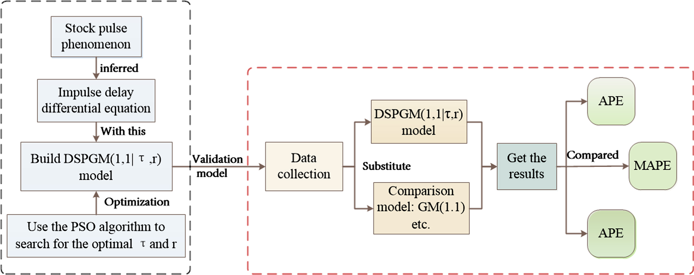
The flow diagram of the DSPGM(1,1|τ,r) model.

5 Applications

Each country’s stock market has its own historical environment and characteristics. China’s stock market is in the development stage, so it is more complex and affected by many factors, making it difficult to predict. Specifically, China’s stock price changes have the following remarkable characteristics:

Stock prices are characterized by large increases and decreases [39]. For example, in 2005, the Shanghai Stock Index rose from the lowest 998 points to 6124 points in only two years, an increase of more than five times. In addition, after the rise, the price collapsed. After reaching a high of 2245 points in 2001, the Shanghai Stock Index dropped 60% to 998 points in 2005. The same situation occurred in 2015, when the Shanghai Stock Index suddenly plunged more than 50% after reaching a high of 5178. For a single stock, it is more common that it rises one day and falls the next. Stock price fluctuations present the typical characteristics of policies. National regulation in some aspects will affect the stock price and be greatly influenced by the mainstream media, which further aggravates the problem of stock price instability.

Therefore, the development of a scientific prediction model is of great importance to individuals, enterprises and countries. In this section, the DSPGM(1,1|τ,r) model is applied to the Shanghai and Shenzhen Stock Indexes and forecasts the individual stocks of Kweichow Moutai and AIER Eye Hospital. The data to establish the model came from Sohu Stocks.

5.1 Example 1: Shanghai Index net forecast

In this case, on the Shanghai composite index, to predict the net value of the daily closing quotation, the data are chosen from between June 29 and July 31, 2020. There are 15 working days (during closed days the net value will not change so it is not studied), denoted by x⁽⁰⁾ (k) , k = 1, 2 ⋯ 25. The actual data are shown in Table 3 (refer to the details in the Appendix, Table 3). Between June 29 and July 17, 15 data points are used to establish the model and between July 20 and July 31, 10 data points are used to test the forecast.

Table 3
The simulation and prediction results of six models on Shanghai Stock Exchange Index

Date Actual ARIMA Verhuls DGM(1,1) NGBM(1,1) WGM(1,1) DSPGM(1,1|τ,r)

values Values APE(%) Values APE(%) Values APE(%) Values APE(%) Values APE(%) Values APE(%)

6.29 2961.5200 2961.5200 0.0000 2961.5200 0.0000 2961.5200 0.0000 2961.5200 0.0000

6.3 2984.6700 2951.0902 1.1251 3013.7354 0.9738 3136.8986 5.1003 2973.2630 0.3822

7.1 3025.9800 3005.8816 0.6642 3060.4754 1.1400 3157.2169 4.3370 3106.5733 2.6634 3320.2583 9.7251 3041.6860 0.5372

7.2 3090.5700 3066.6863 0.7728 3102.1491 0.3747 3177.6669 2.8182 3188.1692 3.1580 3028.1184 2.0207 3107.1724 1.0058

7.3 3152.8100 3084.0434 2.1811 3139.1748 0.4325 3198.2493 1.4412 3242.9366 2.8586 3363.9660 6.6974 3184.5207 2.4219

7.6 3332.8800 3113.7357 6.5752 3171.9681 4.8280 3218.9651 3.4179 3281.0523 1.5550 3072.0868 7.8249 3252.1601 1.4269

7.7 3345.3400 3203.3981 4.2430 3200.9323 4.3167 3239.8150 3.1544 3307.7623 1.1233 3408.1966 1.8789 3393.0742 0.3211

7.8 3403.4400 3345.6859 1.6969 3226.4519 5.2003 3260.8000 4.1911 3326.1526 2.2709 3116.5814 8.4285 3392.5127 0.8121

7.9 3450.5900 3336.8137 3.2973 3248.8880 5.8454 3281.9209 4.8881 3338.2033 3.2570 3452.9566 0.0686 3422.5670 1.5939

7.10 3383.3200 3248.3002 3.9907 3268.5758 3.3915 3303.1786 2.3687 3345.2660 1.1248 3161.6084 6.5531 3437.2472 2.2233

7.13 3443.2900 3340.5343 2.9842 3285.8231 4.5732 3324.5740 3.4477 3348.3071 2.7585 3498.2523 1.5962 3366.7369 0.5800

7.14 3414.6200 3380.1139 1.0105 3300.9104 3.3301 3346.1080 2.0064 3348.0436 1.9497 3207.1742 6.0752 3394.8155 0.2341

7.15 3361.3000 3374.8524 0.4032 3314.0914 1.4045 3367.7814 0.1928 3345.0229 0.4843 3544.0899 5.4381 3353.4305 2.7994

7.16 3210.1000 3325.0785 3.5818 3325.5941 3.5978 3389.5953 5.5916 3339.6729 4.0364 3253.2854 1.3453 3299.9643 0.8267

7.17 3214.1300 3287.4545 2.2813 3335.6223 3.7799 3411.5504 6.1423 3332.3351 3.6777 3590.4762 11.7091 3187.5584 0.5190

MAPE(%) 2.3205 3.0849 3.5070 2.0866 5.3355 1.1770

7.20 3314.3500 3232.0739 2.4824 3344.3578 0.9054 3324.5740 3.5994 3323.2866 0.2696 3299.9483 0.4345 3205.4436 3.2859

7.21 3320.8900 3276.9411 1.3234 3351.9615 0.9356 3346.1080 4.0651 3312.7554 0.2450 3637.4175 9.5314 3289.5798 0.9428

7.22 3333.1600 3397.7701 1.9384 3358.5757 0.7625 3367.7814 4.3536 3300.9316 0.9669 3347.1697 0.4203 3294.5436 1.1586

7.23 3325.1100 3391.4542 1.9952 3364.3261 1.1794 3389.5953 5.2838 3287.9755 1.1168 3684.9205 10.8210 3302.9298 0.6671

7.24 3196.1700 3342.3688 4.5742 3369.3230 5.4175 3411.5504 10.2406 3274.0234 2.4358 3394.9561 6.2195 3295.8872 3.1199

7.27 3205.2300 3378.2121 5.3969 3373.6633 5.2550 3433.6478 10.6410 3259.1924 1.6836 3732.9921 16.4657 3207.0723 0.0575

7.28 3227.9600 3492.6907 8.2012 3377.4318 4.6305 3455.8882 10.5736 3243.5835 0.4840 3443.3144 6.6715 3233.1726 0.1615

7.29 3294.5500 3494.7269 6.0760 3380.7030 2.6150 3478.2728 9.0404 3227.2849 2.0417 3781.6389 14.7847 3267.7134 0.8146

7.30 3286.8200 3452.0185 5.0261 3383.5415 2.9427 3500.8023 10.0047 3210.3738 2.3258 3492.2514 6.2502 3329.4526 1.2971

7.31 3310.1000 3480.1508 5.1373 3386.0041 2.2931 3523.4777 9.9386 3192.9181 3.5401 3830.8678 15.7327 3330.2801 0.6097

MAPE(%) 4.2151 2.6937 7.7741 4.6409 8.7331 1.2114

R R = 0.6700 0.5123 0.4181 R = 0.8472 0.0594 0.9155

Date	Actual	ARIMA	Verhuls	DGM(1,1)	NGBM(1,1)	WGM(1,1)	DSPGM(1,1\|τ,r)
6.29	2961.5200	2961.5200	0.0000	2961.5200	0.0000	2961.5200	0.0000	2961.5200	0.0000
6.3	2984.6700	2951.0902	1.1251	3013.7354	0.9738	3136.8986	5.1003	2973.2630	0.3822
7.1	3025.9800	3005.8816	0.6642	3060.4754	1.1400	3157.2169	4.3370	3106.5733	2.6634	3320.2583	9.7251	3041.6860	0.5372
7.2	3090.5700	3066.6863	0.7728	3102.1491	0.3747	3177.6669	2.8182	3188.1692	3.1580	3028.1184	2.0207	3107.1724	1.0058
7.3	3152.8100	3084.0434	2.1811	3139.1748	0.4325	3198.2493	1.4412	3242.9366	2.8586	3363.9660	6.6974	3184.5207	2.4219
7.6	3332.8800	3113.7357	6.5752	3171.9681	4.8280	3218.9651	3.4179	3281.0523	1.5550	3072.0868	7.8249	3252.1601	1.4269
7.7	3345.3400	3203.3981	4.2430	3200.9323	4.3167	3239.8150	3.1544	3307.7623	1.1233	3408.1966	1.8789	3393.0742	0.3211
7.8	3403.4400	3345.6859	1.6969	3226.4519	5.2003	3260.8000	4.1911	3326.1526	2.2709	3116.5814	8.4285	3392.5127	0.8121
7.9	3450.5900	3336.8137	3.2973	3248.8880	5.8454	3281.9209	4.8881	3338.2033	3.2570	3452.9566	0.0686	3422.5670	1.5939
7.10	3383.3200	3248.3002	3.9907	3268.5758	3.3915	3303.1786	2.3687	3345.2660	1.1248	3161.6084	6.5531	3437.2472	2.2233
7.13	3443.2900	3340.5343	2.9842	3285.8231	4.5732	3324.5740	3.4477	3348.3071	2.7585	3498.2523	1.5962	3366.7369	0.5800
7.14	3414.6200	3380.1139	1.0105	3300.9104	3.3301	3346.1080	2.0064	3348.0436	1.9497	3207.1742	6.0752	3394.8155	0.2341
7.15	3361.3000	3374.8524	0.4032	3314.0914	1.4045	3367.7814	0.1928	3345.0229	0.4843	3544.0899	5.4381	3353.4305	2.7994
7.16	3210.1000	3325.0785	3.5818	3325.5941	3.5978	3389.5953	5.5916	3339.6729	4.0364	3253.2854	1.3453	3299.9643	0.8267
7.17	3214.1300	3287.4545	2.2813	3335.6223	3.7799	3411.5504	6.1423	3332.3351	3.6777	3590.4762	11.7091	3187.5584	0.5190
MAPE(%)	2.3205	3.0849	3.5070	2.0866	5.3355	1.1770
7.20	3314.3500	3232.0739	2.4824	3344.3578	0.9054	3324.5740	3.5994	3323.2866	0.2696	3299.9483	0.4345	3205.4436	3.2859
7.21	3320.8900	3276.9411	1.3234	3351.9615	0.9356	3346.1080	4.0651	3312.7554	0.2450	3637.4175	9.5314	3289.5798	0.9428
7.22	3333.1600	3397.7701	1.9384	3358.5757	0.7625	3367.7814	4.3536	3300.9316	0.9669	3347.1697	0.4203	3294.5436	1.1586
7.23	3325.1100	3391.4542	1.9952	3364.3261	1.1794	3389.5953	5.2838	3287.9755	1.1168	3684.9205	10.8210	3302.9298	0.6671
7.24	3196.1700	3342.3688	4.5742	3369.3230	5.4175	3411.5504	10.2406	3274.0234	2.4358	3394.9561	6.2195	3295.8872	3.1199
7.27	3205.2300	3378.2121	5.3969	3373.6633	5.2550	3433.6478	10.6410	3259.1924	1.6836	3732.9921	16.4657	3207.0723	0.0575
7.28	3227.9600	3492.6907	8.2012	3377.4318	4.6305	3455.8882	10.5736	3243.5835	0.4840	3443.3144	6.6715	3233.1726	0.1615
7.29	3294.5500	3494.7269	6.0760	3380.7030	2.6150	3478.2728	9.0404	3227.2849	2.0417	3781.6389	14.7847	3267.7134	0.8146
7.30	3286.8200	3452.0185	5.0261	3383.5415	2.9427	3500.8023	10.0047	3210.3738	2.3258	3492.2514	6.2502	3329.4526	1.2971
7.31	3310.1000	3480.1508	5.1373	3386.0041	2.2931	3523.4777	9.9386	3192.9181	3.5401	3830.8678	15.7327	3330.2801	0.6097
MAPE(%)	4.2151	2.6937	7.7741	4.6409	8.7331	1.2114
R	R = 0.6700	0.5123	0.4181	R = 0.8472	0.0594	0.9155

Substituting x⁽⁰⁾ (k) into DSPGM(1,1|τ,r) yielded the optimal value τ = 1, r = 1.0163 by PSO, and the model parameters were $\hat{a} = 0.8667, \hat{b} = - 0.9517, \hat{u} = 264.7784$ . Therefore, the time response formula of the model is as follows:

$\begin{matrix} {\hat{x}}^{(0)} (k) = 0.5295 x^{(1)} (k - 1) - 0.8398 (x^{(1)} (k - 1) \\ + x^{(1)} (k - 3)) + 467 . 2715 k^{1.0163} \end{matrix}$ (23)

The results generated by DSPGM(1,1|τ,r) were compared with the ARIMA [33], Verhulst [34], DGM(1,1) [35], NGBM(1,1) [36], and WGM(1,1) [37] models, and the simulation and prediction results of these models are detailed in Table 3 of the Appendix. To compare the results of the six models more clearly, curve comparison diagrams of the six models and the actual stock price are given in Fig. 2, and the error comparison diagram is shown in Fig. 3.

Fig. 2

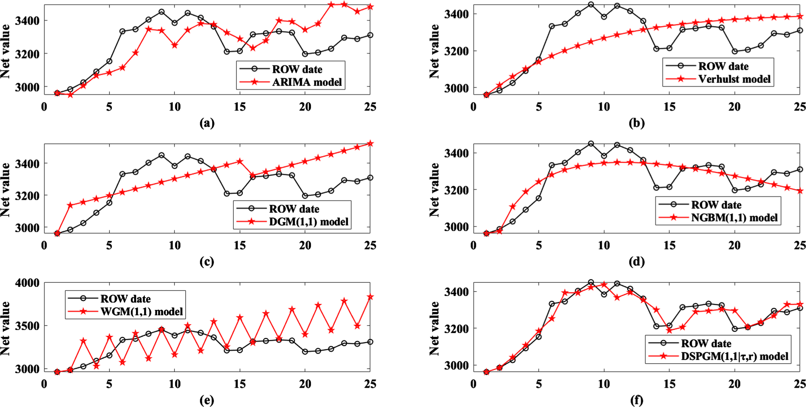
Shanghai Index net change trend charts.

Fig. 3

Error comparison of each model on the Shanghai Stock Exchange Index.

First, Fig. 2 shows six models. The net value of the Shanghai Index prediction results of the DSPGM(1,1|τ,r) model is very similar to the real net value. The remaining models have roughly the same trends, but they all show significant deviations. From the analysis of Table 3 and Fig. 3, it can be found that in the six models, the simulation means absolute percentage error and the prediction mean absolute percentage error of the DSPGM(1,1|τ,r) model are the smallest at 1.1770% and 1.2114%, respectively. The mean prediction errors of the ARIMA [33], traditional Verhulst [34], DGM(1,1) [35] and NGBM(1,1) [36] models are close to each other, at approximately 3%. However, the average prediction errors of the ARIMA, DGM(1,1) [31] and WGM(1,1) [37] models reached more than 7%. Then, looking at the correlation coefficient between the results of each model and the real data in Table 3 and Fig. 2, it can be seen that in the ARIMA, traditional Verhulst, DGM(1,1), NGBM(1,1), WGM(1,1), and DSPGM(1,1|τ,r) models, the fitting results of the Shanghai composite index and the correlation coefficient R of the original data were 0.6700, 0.5123, 0.4181, 0.8472, 0.0594 and 0.9155, respectively. The correlation coefficient between the DSPGM(1,1|τ,r) model and the original data is much higher than that of the others. In summary, it can be concluded that the DSPGM(1,1|τ,r) model is better than the ARIMA model in the prediction of the net value of the Shanghai Composite Index. The traditional Verhulst, DGM(1,1), NGBM(1,1), and WGM(1,1) models

5.2 Example 2: Shenzhen Index net forecast

The results of examples 1 and 2 show that the DSPGM(1,1|τ,r) model has a very high accuracy in the prediction of the Shanghai composite index. To verify that the DSPGM(1,1|τ,r) model can successfully predict China’s stock prices, this example forecasts the net value of the Shenzhen Index.

The daily closing net value of the Shenzhen Index between June 29 and July 31 was selected as x⁽⁰⁾ (k) , k = 1, 2 ⋯ 25, in which 15 sets of data between June 29 and July 17 are used for modelling and 10 sets of data between July 20 and July 31 are used for prediction. x⁽⁰⁾ (k) is substituted into the DSPGM(1,1|τ,r) model. Through a PSO search, the best value τ = 2 and r = 1.034. The results of the model are shown in Table 4 (refer to the details in Appendix 4), the Shenzhen Index net change trend charts are shown in in Fig. 4 and the error comparison of each model to the net forecast of the Shenzhen Index is shown in Fig. 5.

Table 4
The simulation and prediction results of six models on Shenzhen Stock Exchange Index

Date Actual ARIMA Verhuls DGM(1,1) NGBM(1,1) WGM(1,1) DSPGM(1,1|τ,r)

values Values APE(%) Values APE(%) Values APE(%) Values APE(%) Values APE(%) Values APE(%)

6.29 11752.36 11752.3600 0.0000 11752.3600 0.0000 11752.3600 0.0000 11752.3600 0.0000

6.3 11992.35 11974.9394 0.1452 11992.2355 0.0010 12358.6223 3.0542 11697.8221 2.4560

7.1 12112.97 12165.4339 0.4331 12208.3384 0.7873 12472.1958 2.9656 12253.9947 1.1642 12802.9492 5.6962 12112.9700 0

7.2 12269.49 12316.1912 0.3806 12402.1594 1.0813 12586.8129 2.5863 12610.9783 2.7832 12241.3559 0.2293 12394.6087 1.0198

7.3 12433.27 12461.7735 0.2293 12575.3029 1.1424 12702.4833 2.1653 12864.3108 3.4668 13054.0506 4.9929 12623.1780 1.5274

7.6 12941.72 12607.3015 2.5840 12729.4235 1.6404 12819.2168 0.9466 13053.1484 0.8610 12494.5704 3.4551 12851.8944 0.6941

7.7 13163.98 12835.4231 2.4959 12866.1759 2.2623 12937.0230 1.7241 13197.6834 0.2560 13309.3961 1.1047 13192.4245 0.2161

7.8 13406.37 13023.5897 2.8552 12987.1755 3.1268 13055.9118 2.6141 13309.7891 0.7204 12752.0647 4.8806 13441.9845 0.2657

7.9 13754.74 13202.7262 4.0133 13093.9701 4.8039 13175.8932 4.2083 13397.0787 2.6003 13569.0574 1.3500 13590.5444 1.1937

7.10 13671.24 13404.1333 1.9538 13188.0197 3.5346 13296.9771 2.7376 13464.7445 1.5104 13013.9112 4.8081 13748.5257 0.5653

7.13 14149.14 13509.7500 4.5189 13270.6849 6.2085 13419.1739 5.1591 13516.4970 4.4712 13833.1074 2.2336 13722.5909 3.0147

7.14 13996.46 13716.7092 1.9987 13343.2197 4.6672 13542.4936 3.2434 13555.0855 3.1535 13280.1834 5.1176 13806.4880 1.3573

7.15 13734.13 13807.6699 0.5355 13406.7705 2.3835 13666.9465 0.4892 13582.6079 1.1033 14101.6204 2.6757 13733.5324 0.0044

7.16 12996.34 13832.1246 6.4309 13462.3769 3.5859 13792.5432 6.1264 13600.7033 4.6503 13550.9560 4.2675 13482.0201 3.7371

7.17 13114.94 13719.5564 4.6101 13510.9763 3.0197 13919.2941 6.1331 13610.6791 3.7800 14374.6718 9.6053 13079.9895 0.2665

MAPE(%) 2.2123 2.7318 3.1538 2.1984 3.8782 1.1552

7.20 13448.85 13764.7373 2.3488 13553.4090 0.7775 14047.2098 4.4492 13613.5952 1.2250 14106.3084 3.2897 13000.3137 3.3351

7.21 13536.17 13868.5283 2.4553 13590.4251 0.4008 14176.3010 4.7290 13610.3243 0.5478 14934.6977 9.3196 13217.2626 2.3560

7.22 13657.03 13992.6432 2.4574 13622.6913 0.2514 14306.5786 4.7561 13601.5936 0.4059 14391.0441 11.2506 13347.3056 2.2679

7.23 13661.5 14123.8058 3.3840 13650.7984 0.0783 14438.0533 5.6842 13588.0162 0.5379 15221.8296 17.2997 13411.0020 1.8336

7.24 12935.7 14257.4124 10.2176 13675.2683 5.7173 14570.7363 12.6397 13570.1138 4.9044 14680.5924 11.6620 13423.7949 3.7732

7.27 12976.87 14391.8664 10.9040 13696.5610 5.5460 14704.6387 13.3142 13548.3344 4.4037 15513.8146 14.4303 13140.9929 1.2647

7.28 13147.35 14526.6143 10.4908 13715.0807 4.3182 14839.7715 12.8727 13523.0659 2.8577 14975.0346 11.1992 13074.4624 0.5544

7.29 13557.44 14661.4641 8.1433 13731.1825 1.2815 14976.1462 10.4644 13494.6463 0.4632 15810.7347 15.9325 13261.2951 2.1844

7.30 13466.86 14796.3492 9.8723 13745.1774 2.0667 15113.7742 12.2294 13463.3720 0.0259 14106.3084 3.2897 13543.9121 0.5722

7.31 13637.88 14931.2466 9.4836 13757.3375 0.8759 15252.6670 11.8405 13429.5045 1.5279 14934.6977 9.3196 13638.1483 0.0020

MAPE(%) 6.9757 2.1314 9.2979 4.9876 10.5436 1.8143

R 0.6860 0.7013 0.5864 0.8512 0.3913 0.9286

Date	Actual	ARIMA	Verhuls	DGM(1,1)	NGBM(1,1)	WGM(1,1)	DSPGM(1,1\|τ,r)
6.29	11752.36	11752.3600	0.0000	11752.3600	0.0000	11752.3600	0.0000	11752.3600	0.0000
6.3	11992.35	11974.9394	0.1452	11992.2355	0.0010	12358.6223	3.0542	11697.8221	2.4560
7.1	12112.97	12165.4339	0.4331	12208.3384	0.7873	12472.1958	2.9656	12253.9947	1.1642	12802.9492	5.6962	12112.9700	0
7.2	12269.49	12316.1912	0.3806	12402.1594	1.0813	12586.8129	2.5863	12610.9783	2.7832	12241.3559	0.2293	12394.6087	1.0198
7.3	12433.27	12461.7735	0.2293	12575.3029	1.1424	12702.4833	2.1653	12864.3108	3.4668	13054.0506	4.9929	12623.1780	1.5274
7.6	12941.72	12607.3015	2.5840	12729.4235	1.6404	12819.2168	0.9466	13053.1484	0.8610	12494.5704	3.4551	12851.8944	0.6941
7.7	13163.98	12835.4231	2.4959	12866.1759	2.2623	12937.0230	1.7241	13197.6834	0.2560	13309.3961	1.1047	13192.4245	0.2161
7.8	13406.37	13023.5897	2.8552	12987.1755	3.1268	13055.9118	2.6141	13309.7891	0.7204	12752.0647	4.8806	13441.9845	0.2657
7.9	13754.74	13202.7262	4.0133	13093.9701	4.8039	13175.8932	4.2083	13397.0787	2.6003	13569.0574	1.3500	13590.5444	1.1937
7.10	13671.24	13404.1333	1.9538	13188.0197	3.5346	13296.9771	2.7376	13464.7445	1.5104	13013.9112	4.8081	13748.5257	0.5653
7.13	14149.14	13509.7500	4.5189	13270.6849	6.2085	13419.1739	5.1591	13516.4970	4.4712	13833.1074	2.2336	13722.5909	3.0147
7.14	13996.46	13716.7092	1.9987	13343.2197	4.6672	13542.4936	3.2434	13555.0855	3.1535	13280.1834	5.1176	13806.4880	1.3573
7.15	13734.13	13807.6699	0.5355	13406.7705	2.3835	13666.9465	0.4892	13582.6079	1.1033	14101.6204	2.6757	13733.5324	0.0044
7.16	12996.34	13832.1246	6.4309	13462.3769	3.5859	13792.5432	6.1264	13600.7033	4.6503	13550.9560	4.2675	13482.0201	3.7371
7.17	13114.94	13719.5564	4.6101	13510.9763	3.0197	13919.2941	6.1331	13610.6791	3.7800	14374.6718	9.6053	13079.9895	0.2665
MAPE(%)	2.2123	2.7318	3.1538	2.1984	3.8782	1.1552
7.20	13448.85	13764.7373	2.3488	13553.4090	0.7775	14047.2098	4.4492	13613.5952	1.2250	14106.3084	3.2897	13000.3137	3.3351
7.21	13536.17	13868.5283	2.4553	13590.4251	0.4008	14176.3010	4.7290	13610.3243	0.5478	14934.6977	9.3196	13217.2626	2.3560
7.22	13657.03	13992.6432	2.4574	13622.6913	0.2514	14306.5786	4.7561	13601.5936	0.4059	14391.0441	11.2506	13347.3056	2.2679
7.23	13661.5	14123.8058	3.3840	13650.7984	0.0783	14438.0533	5.6842	13588.0162	0.5379	15221.8296	17.2997	13411.0020	1.8336
7.24	12935.7	14257.4124	10.2176	13675.2683	5.7173	14570.7363	12.6397	13570.1138	4.9044	14680.5924	11.6620	13423.7949	3.7732
7.27	12976.87	14391.8664	10.9040	13696.5610	5.5460	14704.6387	13.3142	13548.3344	4.4037	15513.8146	14.4303	13140.9929	1.2647
7.28	13147.35	14526.6143	10.4908	13715.0807	4.3182	14839.7715	12.8727	13523.0659	2.8577	14975.0346	11.1992	13074.4624	0.5544
7.29	13557.44	14661.4641	8.1433	13731.1825	1.2815	14976.1462	10.4644	13494.6463	0.4632	15810.7347	15.9325	13261.2951	2.1844
7.30	13466.86	14796.3492	9.8723	13745.1774	2.0667	15113.7742	12.2294	13463.3720	0.0259	14106.3084	3.2897	13543.9121	0.5722
7.31	13637.88	14931.2466	9.4836	13757.3375	0.8759	15252.6670	11.8405	13429.5045	1.5279	14934.6977	9.3196	13638.1483	0.0020
MAPE(%)	6.9757	2.1314	9.2979	4.9876	10.5436	1.8143
R	0.6860	0.7013	0.5864	0.8512	0.3913	0.9286

Fig. 4

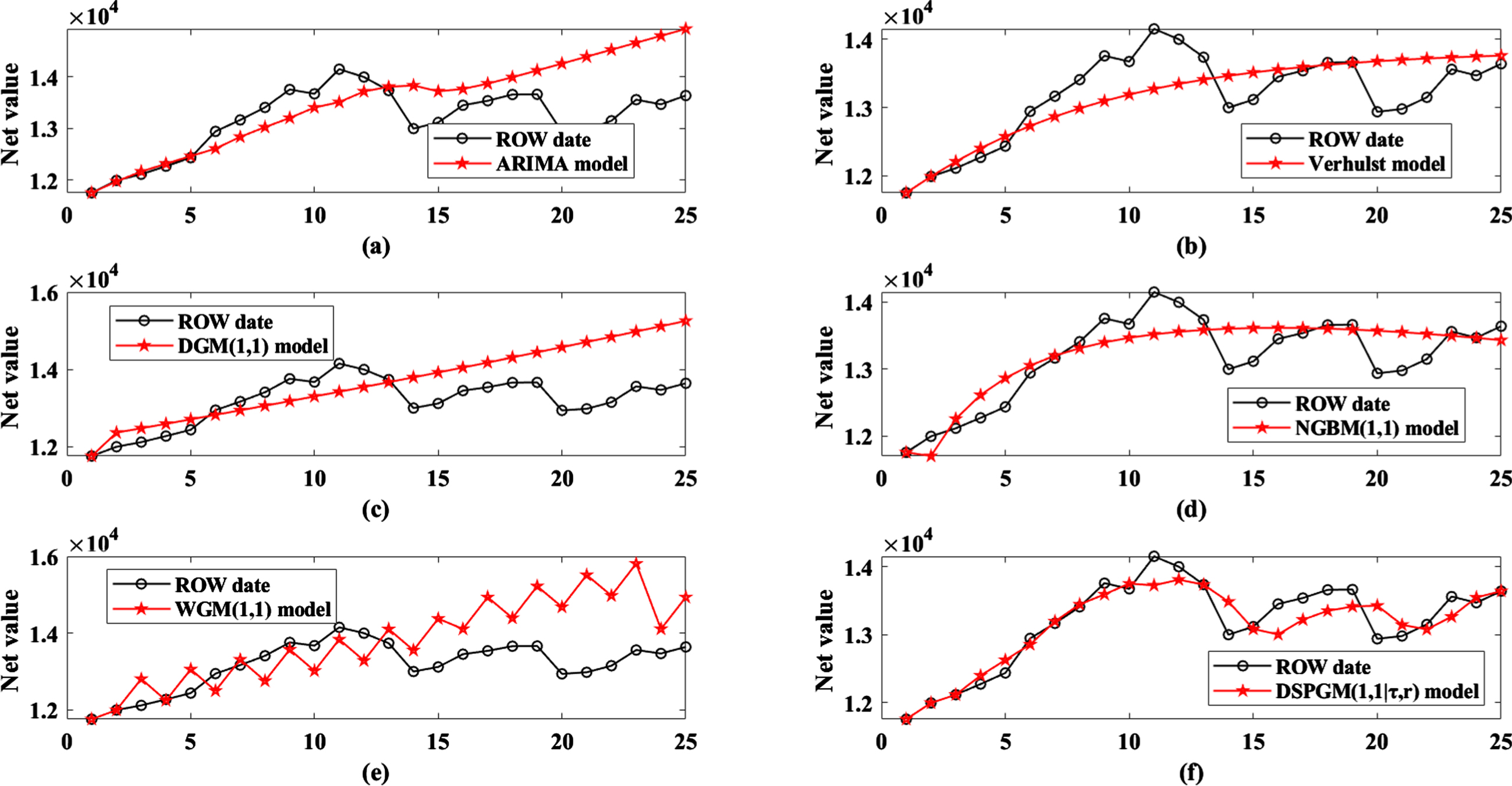
Shenzhen Index net change trend charts.

Fig. 5

Error comparison of each model on the Shenzhen Index.

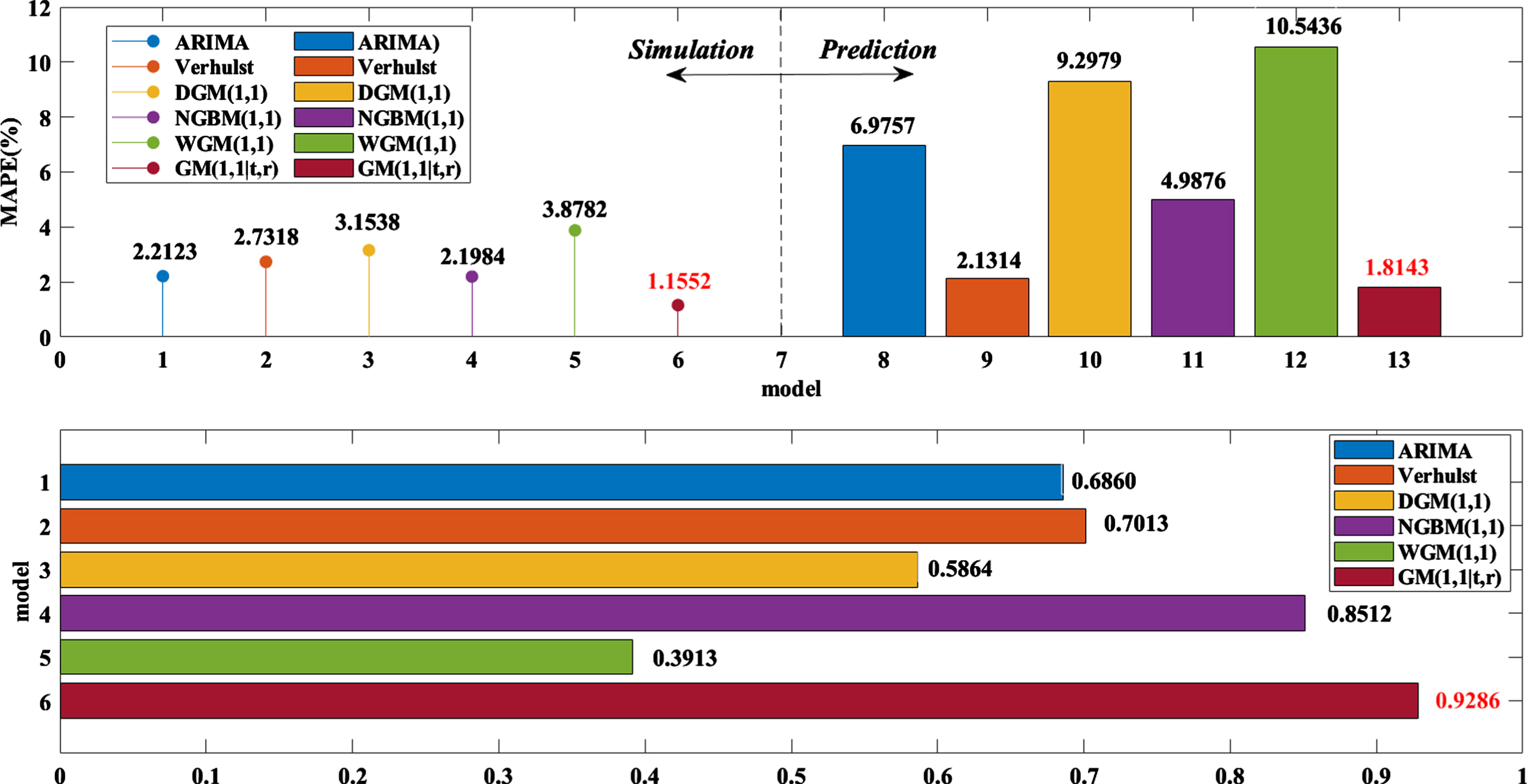
Figure 4 shows the changes in the predicted values of the six models and the true values of the net value of the Shenzhen Index. Obviously, the predicted value curve of the DSPGM(1,1|τ,r) model is closest to the true value of the net value of the Shenzhen Index. The DGM(1,1) and WGM(1,1) models are the worst. The specific results can be seen in Table 4 and Fig. 5. In the simulation and prediction of the Shenzhen Index, the simulation error of the DSPGM(1,1|τ,r) model is 1.1552% and the prediction error is 1.8143%, which are lower than those of the comparison models. The WGM(1,1) model has the worst results; its simulation error is 3.8782% and its prediction error is 10.5436%, which are higher than those of the DSPGM(1,1|τ,r) model by over 2% and 8%, respectively. The simulation errors of the Verhulst, DGM(1,1) and NGBM(1,1) models are close to 3%, but the prediction error of the DGM(1,1) model is 9.2979%. The Verhulst and NGBM(1,1) models are 2.1314% and 4.9876%, respectively.

Then, look at the correlation coefficient between the results of each model and the real data as shown in Table 4 and Fig. 6, which show that in the ARIMA, traditional Verhulst, DGM(1,1), NGBM(1,1), WGM(1,1), and DSPGM(1,1|τ,r) models, the fitting results of the Shanghai composite index and the correlation coefficient R of the original data were 0.6860, 0.7013, 0.5864, 0.8512, 0.3913, and 0.9286, respectively. The correlation coefficient between the DSPGM(1,1|τ,r) model and the original data is much higher than that of the others. It can be concluded that the DSPGM(1,1|τ,r) model is better than the ARIMA, traditional Verhulst, DGM(1,1), NGBM(1,1), and WGM(1,1) models in the CSI 300 index net forecast. Again, the effectiveness of the DSPGM(1,1|τ,r) model was proven.

Fig. 6

Kweichow Moutai net change trend charts.

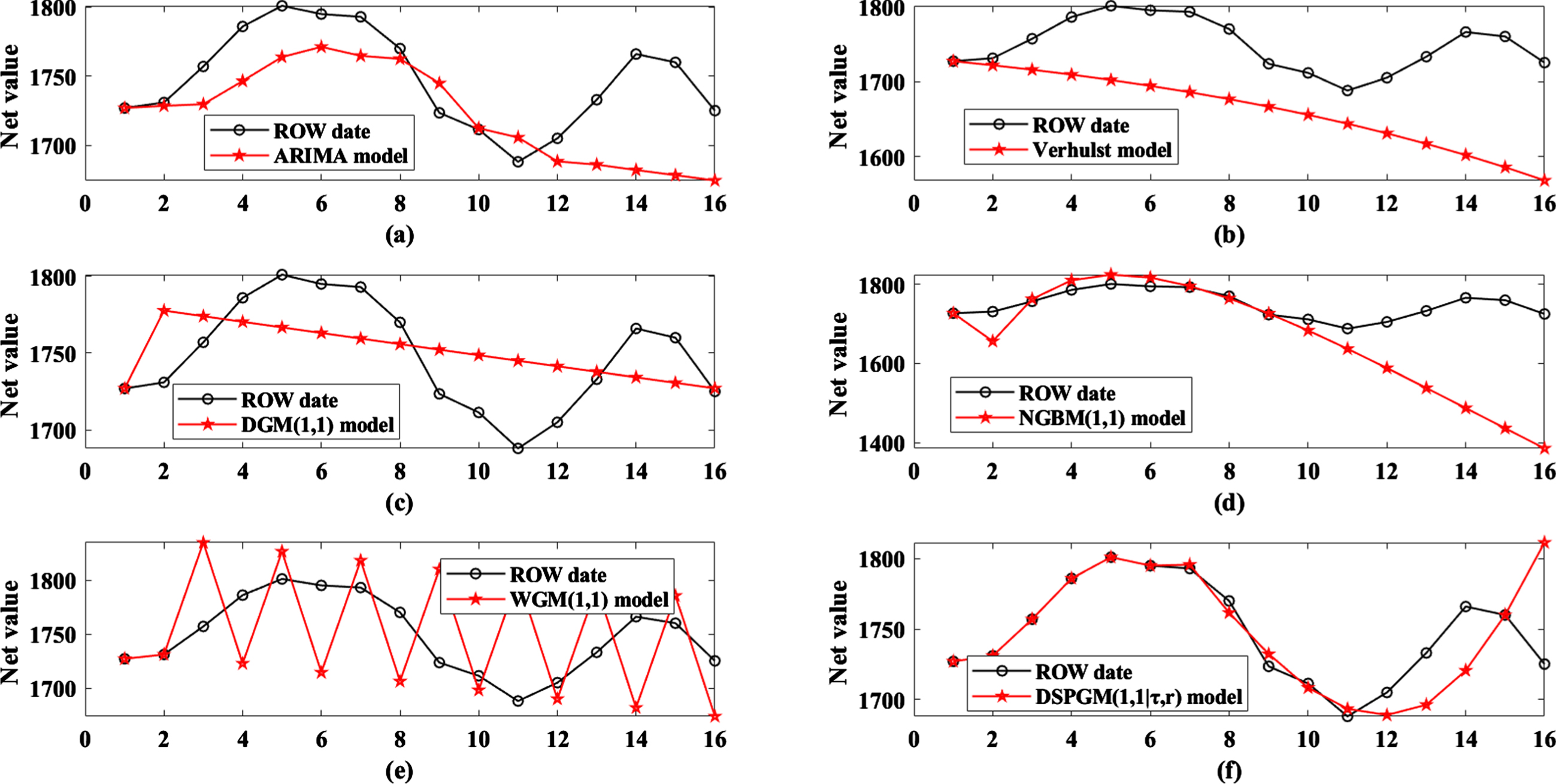
5.3 Example 3: Kweichow Moutai net forecast

This case selects Kweichow Moutai, a typical stock in the Shanghai Stock Exchange Index, and simulates and forecasts its net value to supplement the prediction conclusion of the Shanghai Stock Exchange Index. This shows that the accurate effect of the model is not due to chance. Data from 16 working days between August 26 and September 17, 2020, are selected and denoted as x⁽⁰⁾ (k) , k = 1, 2 ⋯ 16. The actual data are shown in Table 5 (refer to the details in the Appendix, Table 5), of which 10 sets of data between August 26 and September 9 are used to establish the model and 6 sets of data between September 10 and September 16 are used for the prediction test.

Table 5
The simulation and prediction results of six models on Kweichow Moutai

Date Actual ARIMA Verhuls DGM(1,1) NGBM(1,1) WGM(1,1) DSPGM(1,1|τ,r)

values Values APE(%) Values APE(%) Values APE(%) Values APE(%) Values APE(%) Values APE(%)

8.26 1727.0000 1727.0000 0.0000 1727.0000 0.0000 1727.0000 0.0000 1727.0000 0.0000

8.27 1731.0000 1728.5655 0.1406 1721.5617 0.5452 1777.6715 2.6962 1656.0838 4.3279

8.28 1757.0000 1729.7494 1.5510 1715.6120 2.3556 1774.0112 0.9682 1762.9122 0.3365 1834.5311 4.4125

8.31 1786.0000 1746.5534 2.2087 1709.1069 4.3053 1770.3583 0.8758 1810.2921 1.3601 1722.7196 3.5431

9.1 1801.0000 1763.8670 2.0618 1701.9995 5.4970 1766.7130 1.9038 1824.2665 1.2919 1826.2686 1.4029

9.2 1795.0000 1771.2129 1.3252 1694.2402 5.6134 1763.0752 1.7785 1817.1060 1.2315 1714.4750 4.4860 1795.0000 0.0000

9.3 1793.0000 1764.7172 1.5774 1685.7761 5.9801 1759.4449 1.8714 1795.7433 0.1530 1818.0417 1.3966 1795.6965 0.1504

9.4 1770.0000 1762.4854 0.4246 1676.5519 5.2796 1755.8221 0.8010 1764.5290 0.3091 1706.2659 3.6006 1761.5901 0.4751

9.7 1723.5000 1744.9404 1.2440 1666.5092 3.3067 1752.2067 1.6656 1726.3853 0.1674 1809.8504 5.0102 1732.2408 0.5072

9.8 1711.4000 1712.3359 0.0547 1655.5873 3.2612 1748.5988 2.1736 1683.3696 1.6379 1698.0923 0.7773 1708.3739 0.1768

MAPE(%) 1.0576 4.1600 1.6371 1.0815 0.3078 0.3274

9.9 1688.0000 1705.6508 1.0457 1643.7234 2.6230 1744.9983 3.3767 1636.9792 3.0226 1801.6944 6.7356 1693.3755 0.3185

9.10 1705.0000 1688.2829 0.1294 1630.8526 4.3488 1741.4052 2.1352 1588.3314 6.8427 1689.9539 0.8821 1688.9563 0.9410

9.11 1733.0000 1685.9269 1.1801 1616.9091 6.6988 1737.8195 0.2781 1538.2741 11.2363 1793.5736 3.4955 1696.2544 2.1203

9.14 1766.0000 1682.0187 3.3547 1601.8262 9.2964 1734.2412 1.7983 1487.4598 15.7724 1681.8506 4.7645 1720.5848 2.5716

9.15 1760.0000 1678.2711 2.8181 1585.5375 9.9126 1730.6703 1.6665 1436.3947 18.3867 1785.4879 1.4486 1759.9522 0.0027

9.16 1725.1000 1674.5068 1.1044 1567.9776 9.1080 1727.1067 0.1163 1385.4735 19.6873 1673.7823 2.9741 1811.3556 5.0000

MAPE(%) 3.2057 6.9980 1.5619 14.2939 3.8446 1.8257

R 0.5993 0.2066 0.4424 0.4597 0.1467 0.6753

Date	Actual	ARIMA	Verhuls	DGM(1,1)	NGBM(1,1)	WGM(1,1)	DSPGM(1,1\|τ,r)
8.26	1727.0000	1727.0000	0.0000	1727.0000	0.0000	1727.0000	0.0000	1727.0000	0.0000
8.27	1731.0000	1728.5655	0.1406	1721.5617	0.5452	1777.6715	2.6962	1656.0838	4.3279
8.28	1757.0000	1729.7494	1.5510	1715.6120	2.3556	1774.0112	0.9682	1762.9122	0.3365	1834.5311	4.4125
8.31	1786.0000	1746.5534	2.2087	1709.1069	4.3053	1770.3583	0.8758	1810.2921	1.3601	1722.7196	3.5431
9.1	1801.0000	1763.8670	2.0618	1701.9995	5.4970	1766.7130	1.9038	1824.2665	1.2919	1826.2686	1.4029
9.2	1795.0000	1771.2129	1.3252	1694.2402	5.6134	1763.0752	1.7785	1817.1060	1.2315	1714.4750	4.4860	1795.0000	0.0000
9.3	1793.0000	1764.7172	1.5774	1685.7761	5.9801	1759.4449	1.8714	1795.7433	0.1530	1818.0417	1.3966	1795.6965	0.1504
9.4	1770.0000	1762.4854	0.4246	1676.5519	5.2796	1755.8221	0.8010	1764.5290	0.3091	1706.2659	3.6006	1761.5901	0.4751
9.7	1723.5000	1744.9404	1.2440	1666.5092	3.3067	1752.2067	1.6656	1726.3853	0.1674	1809.8504	5.0102	1732.2408	0.5072
9.8	1711.4000	1712.3359	0.0547	1655.5873	3.2612	1748.5988	2.1736	1683.3696	1.6379	1698.0923	0.7773	1708.3739	0.1768
MAPE(%)	1.0576	4.1600	1.6371	1.0815	0.3078	0.3274
9.9	1688.0000	1705.6508	1.0457	1643.7234	2.6230	1744.9983	3.3767	1636.9792	3.0226	1801.6944	6.7356	1693.3755	0.3185
9.10	1705.0000	1688.2829	0.1294	1630.8526	4.3488	1741.4052	2.1352	1588.3314	6.8427	1689.9539	0.8821	1688.9563	0.9410
9.11	1733.0000	1685.9269	1.1801	1616.9091	6.6988	1737.8195	0.2781	1538.2741	11.2363	1793.5736	3.4955	1696.2544	2.1203
9.14	1766.0000	1682.0187	3.3547	1601.8262	9.2964	1734.2412	1.7983	1487.4598	15.7724	1681.8506	4.7645	1720.5848	2.5716
9.15	1760.0000	1678.2711	2.8181	1585.5375	9.9126	1730.6703	1.6665	1436.3947	18.3867	1785.4879	1.4486	1759.9522	0.0027
9.16	1725.1000	1674.5068	1.1044	1567.9776	9.1080	1727.1067	0.1163	1385.4735	19.6873	1673.7823	2.9741	1811.3556	5.0000
MAPE(%)	3.2057	6.9980	1.5619	14.2939	3.8446	1.8257
R	0.5993	0.2066	0.4424	0.4597	0.1467	0.6753

According to Section 4.2, the delay factor τ = 5 and the nonlinear factor r = 1.2035. The results are shown in Table 4, which uses the ARIMA, traditional Verhulst, DGM(1,1), NGBM(1,1), and WGM(1,1) models to forecast Kweichow Moutai’s net worth. Then, the results generated by the DSPGM(1,1|τ,r) model are compared to them; the results are presented in Table 5, titled “The simulation and prediction results of six models on Kweichow Moutai index”, Fig. 6, titled “Kweichow Moutai net change trend charts”, and Fig. 7, titled “Error comparison of each model on Kweichow Moutai”.

Fig. 7

Error comparison of each model on Kweichow Moutai.

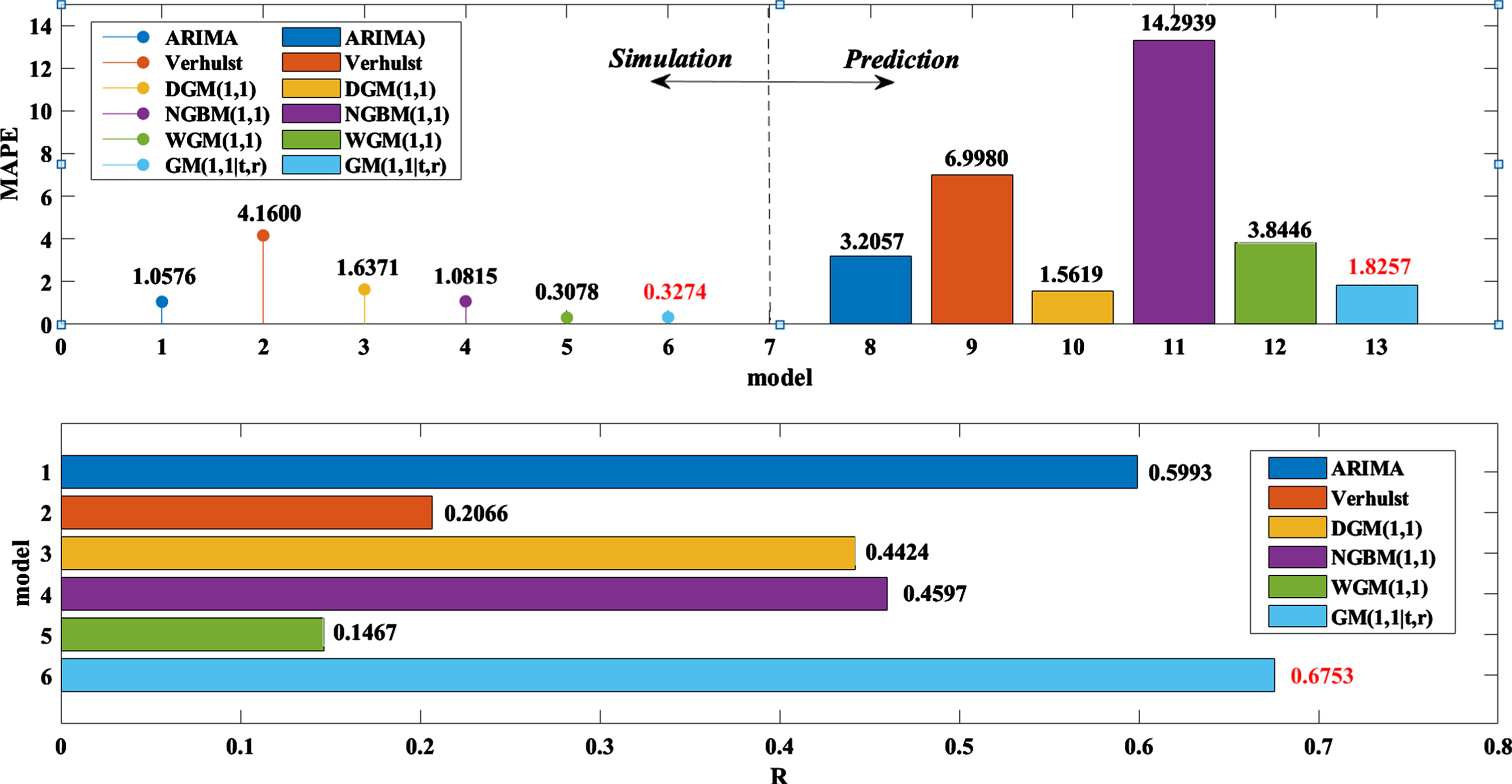
Figure 6 shows the changes in the predicted values of the six models and the true values of the net value of Kweichow Moutai. Obviously, the predicted value curve of the DSPGM(1,1|τ,r) model is closest to the true value, but other models have a large error relative to the real value. The specific results can be seen in Table 5 and Fig. 7. The simulation error of the DSPGM(1,1|τ,r) model is 0.3972% and the prediction error is 1.8257%, so it has very good prediction results. In the other models, the simulation error of the traditional Verhulst model is 4.16%, which is the highest of the six models, but its prediction error is 14.2939%. The prediction error of the NGBM(1,1) model is 14.2939%, which is more than 10%, so it does not fit the forecast of the Kweichow Moutai stock price. The simulation errors of the ARIMA, DGM(1,1) and WGM(1,1) models are approximately 1% and their prediction errors are approximately 2%, which is higher than that of the DSPGM(1,1|τ,r) model.

Then, look at the correlation coefficient between the results of each model and the real data. Table 5 and Fig. 7 show that in the ARIMA, traditional Verhulst, DGM(1,1), NGBM(1,1), WGM(1,1), and DSPGM(1,1|τ,r) models, the fitting results of the Shanghai composite index and the correlation coefficient R of the original data were 0.5993, 0.2066, 0.4424, 0.4597, 0.1467, and 0.6753, respectively. The correlation coefficient between the DSPGM(1,1|τ,r) model and the original data is much higher than that of the others. In summary, DSPGM(1,1|τ,r) is better than the ARIMA, traditional Verhulst, DGM(1,1), NGBM(1,1), and WGM(1,1) models in the forecasting of Kweichow Moutai.

5.4 Example 4: AIER Eye Hospital net forecast

AIER Eye Hospital is a typical stock listed on the Shenzhen Index Stock Exchange. This case is to predict its net worth. The daily closing net value of AIER Eye Hospital between August 25 and September 7, 2020, is selected for modelling; there are 10 sets of data. The other 9 sets of data between September 8 to 9 September 18 are used for prediction. They are denoted by x⁽⁰⁾ (k) , k = 1, 2 ⋯ 19 and substituted into the DSPGM(1,1|τ,r) model. Through the PSO search, the best values τ = 3 and r = 0.9398. The results of the model are shown in Table 6 (refer to the details in the Appendix, Table 6). Figure 8 presents the AIER Eye Hospital net change trend charts and Fig. 9 shows the error comparison of each model on the net forecast of AIER Eye Hospital.

Table 6
The simulation and prediction results of six models on AIER Eye Hospital

Date Actual ARIMA Verhuls DGM(1,1) NGBM(1,1) WGM(1,1) DSPGM(1,1|τ,r)

values Values APE(%) Values APE(%) Values APE(%) Values APE(%) Values APE(%) Values APE(%)

8.25 46.3500 45.2885 2.2903 46.3500 0.0000 46.3500 0.0000 46.3500 0.0000

8.26 49.9800 49.1296 1.7014 49.1644 1.6318 50.6193 1.2790 46.8631 6.2363

8.27 50.5100 50.8349 0.6432 50.8858 0.7441 51.0155 1.0008 50.5307 0.0410 51.7517 2.4584

8.28 51.2300 50.6775 1.0785 51.8981 1.3042 51.4149 0.3609 52.4836 2.4470 50.7992 0.8408 51.2300 0.0000

8.31 51.9700 51.8921 0.1499 52.4798 0.9809 51.8174 0.2937 53.4662 2.8790 52.5767 1.1675 51.8953 0.1437

9.1 53.7300 52.2617 2.7327 52.8095 1.7132 52.2230 2.8047 53.8235 0.1740 51.6301 3.9083 53.4726 0.4790

9.2 53.4300 54.2208 1.4801 52.9950 0.8142 52.6318 1.4938 53.7487 0.5965 53.4134 0.0311 53.7117 0.5272

9.3 53.6500 53.0437 1.1300 53.0989 1.0272 53.0439 1.1298 53.3630 0.5349 52.4726 2.1946 53.6148 0.0657

9.4 52.5000 54.3839 3.5884 53.1570 1.2514 53.4591 1.8269 52.7479 0.4722 54.2619 3.3559 53.0432 1.0347

9.7 53.1000 45.2885 2.2903 53.1894 0.1683 53.8776 1.4644 51.9612 2.1447 53.3270 0.4275 52.6326 0.8803

MAPE(%) 1.5516 1.0706 1.2948 1.5526 1.7980 0.5218

9.8 51.0300 52.7171 0.7212 53.2074 4.2670 53.8776 6.4068 51.0451 0.0297 55.1223 4.0923 51.6329 1.1814

9.9 50.0600 54.7598 7.3090 53.2175 6.3075 54.2994 9.3177 50.0320 0.0559 54.1935 4.1335 51.2319 2.3410

9.10 49.0200 55.8703 11.6068 53.2231 8.5743 54.7245 12.5109 48.9465 0.1499 55.9949 6.9749 50.9829 4.0043

9.11 49.0200 56.1823 14.6110 53.2263 8.5807 55.1529 13.3917 47.8081 2.4722 55.0722 6.0522 50.9239 3.8839

9.14 49.8500 56.9981 16.2753 53.2280 6.7763 55.5846 12.3766 46.6323 6.4547 56.8798 7.0298 50.5925 1.4895

9.15 49.6600 57.4961 15.3381 53.2290 7.1868 56.0197 13.6897 45.4316 8.5148 55.9634 6.3034 49.6602 0.0003

9.16 49.7800 58.1946 17.1860 53.2295 6.9295 56.4583 14.3034 44.2159 11.1774 57.7772 7.9972 48.6046 2.3611

9.17 46.6700 58.7665 18.0525 53.2298 14.0557 56.9003 22.8748 42.9935 7.8776 56.8671 10.1971 47.3353 1.4254

9.18 47.6000 59.4183 27.3159 53.2300 11.8277 57.3457 21.4172 41.7712 12.2454 58.6872 11.0872 47.2735 0.6860

MAPE(%) 17.0874 8.2784 14.0320 7.1670 14.5393 1.9303

R 0.2133 0.3550 0.1709 0.8642 0.7351 0.9178

Date	Actual	ARIMA	Verhuls	DGM(1,1)	NGBM(1,1)	WGM(1,1)	DSPGM(1,1\|τ,r)
8.25	46.3500	45.2885	2.2903	46.3500	0.0000	46.3500	0.0000	46.3500	0.0000
8.26	49.9800	49.1296	1.7014	49.1644	1.6318	50.6193	1.2790	46.8631	6.2363
8.27	50.5100	50.8349	0.6432	50.8858	0.7441	51.0155	1.0008	50.5307	0.0410	51.7517	2.4584
8.28	51.2300	50.6775	1.0785	51.8981	1.3042	51.4149	0.3609	52.4836	2.4470	50.7992	0.8408	51.2300	0.0000
8.31	51.9700	51.8921	0.1499	52.4798	0.9809	51.8174	0.2937	53.4662	2.8790	52.5767	1.1675	51.8953	0.1437
9.1	53.7300	52.2617	2.7327	52.8095	1.7132	52.2230	2.8047	53.8235	0.1740	51.6301	3.9083	53.4726	0.4790
9.2	53.4300	54.2208	1.4801	52.9950	0.8142	52.6318	1.4938	53.7487	0.5965	53.4134	0.0311	53.7117	0.5272
9.3	53.6500	53.0437	1.1300	53.0989	1.0272	53.0439	1.1298	53.3630	0.5349	52.4726	2.1946	53.6148	0.0657
9.4	52.5000	54.3839	3.5884	53.1570	1.2514	53.4591	1.8269	52.7479	0.4722	54.2619	3.3559	53.0432	1.0347
9.7	53.1000	45.2885	2.2903	53.1894	0.1683	53.8776	1.4644	51.9612	2.1447	53.3270	0.4275	52.6326	0.8803
MAPE(%)	1.5516	1.0706	1.2948	1.5526	1.7980	0.5218
9.8	51.0300	52.7171	0.7212	53.2074	4.2670	53.8776	6.4068	51.0451	0.0297	55.1223	4.0923	51.6329	1.1814
9.9	50.0600	54.7598	7.3090	53.2175	6.3075	54.2994	9.3177	50.0320	0.0559	54.1935	4.1335	51.2319	2.3410
9.10	49.0200	55.8703	11.6068	53.2231	8.5743	54.7245	12.5109	48.9465	0.1499	55.9949	6.9749	50.9829	4.0043
9.11	49.0200	56.1823	14.6110	53.2263	8.5807	55.1529	13.3917	47.8081	2.4722	55.0722	6.0522	50.9239	3.8839
9.14	49.8500	56.9981	16.2753	53.2280	6.7763	55.5846	12.3766	46.6323	6.4547	56.8798	7.0298	50.5925	1.4895
9.15	49.6600	57.4961	15.3381	53.2290	7.1868	56.0197	13.6897	45.4316	8.5148	55.9634	6.3034	49.6602	0.0003
9.16	49.7800	58.1946	17.1860	53.2295	6.9295	56.4583	14.3034	44.2159	11.1774	57.7772	7.9972	48.6046	2.3611
9.17	46.6700	58.7665	18.0525	53.2298	14.0557	56.9003	22.8748	42.9935	7.8776	56.8671	10.1971	47.3353	1.4254
9.18	47.6000	59.4183	27.3159	53.2300	11.8277	57.3457	21.4172	41.7712	12.2454	58.6872	11.0872	47.2735	0.6860
MAPE(%)	17.0874	8.2784	14.0320	7.1670	14.5393	1.9303
R	0.2133	0.3550	0.1709	0.8642	0.7351	0.9178

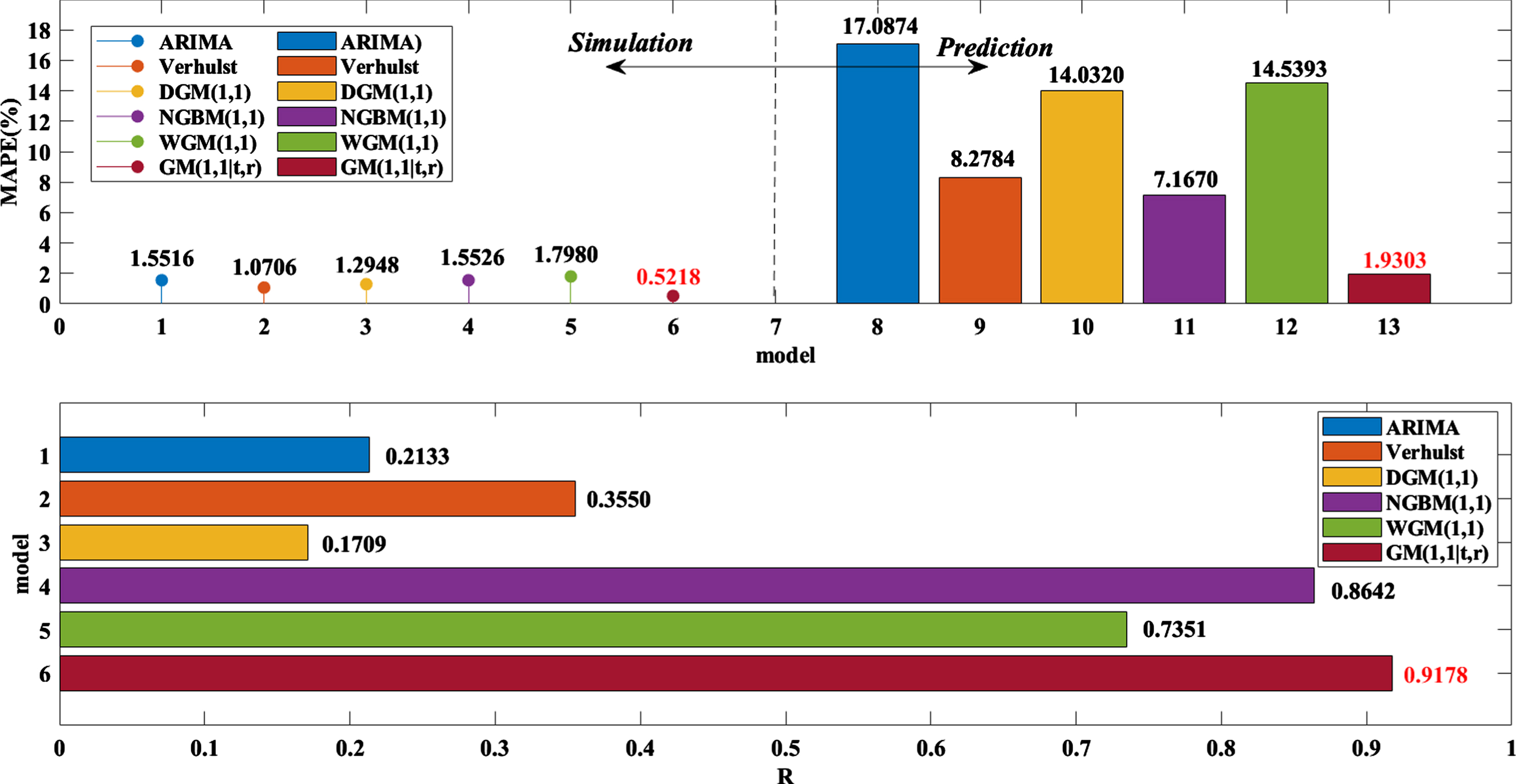
Figure 8 shows the changes in the predicted values of the six models and the true values of the net value of the AIER Eye Hospital. The predicted value curve of the DSPGM(1,1|τ,r) model has a very similar trend to the true value. However, the results of the ARIMA, traditional Verhulst, DGM(1,1) and WGM(1,1) models are increasingly higher than the real price. The results of the NGBM(1,1) model are gradually lower than the real price. These results show the effectiveness of the DSPGM(1,1|τ,r) model. The specific results can be seen in Table 6 and Fig. 8. The simulation error of the DSPGM(1,1|τ,r) model is 0.5218% and its prediction error is 1.903%. For the comparison models, their simulation errors are approximately 1.5%, but all have a large prediction error. The smallest prediction error is 7.1670%, which is five percentage points higher than that of the DSPGM(1,1|τ,r) model.

Fig. 8

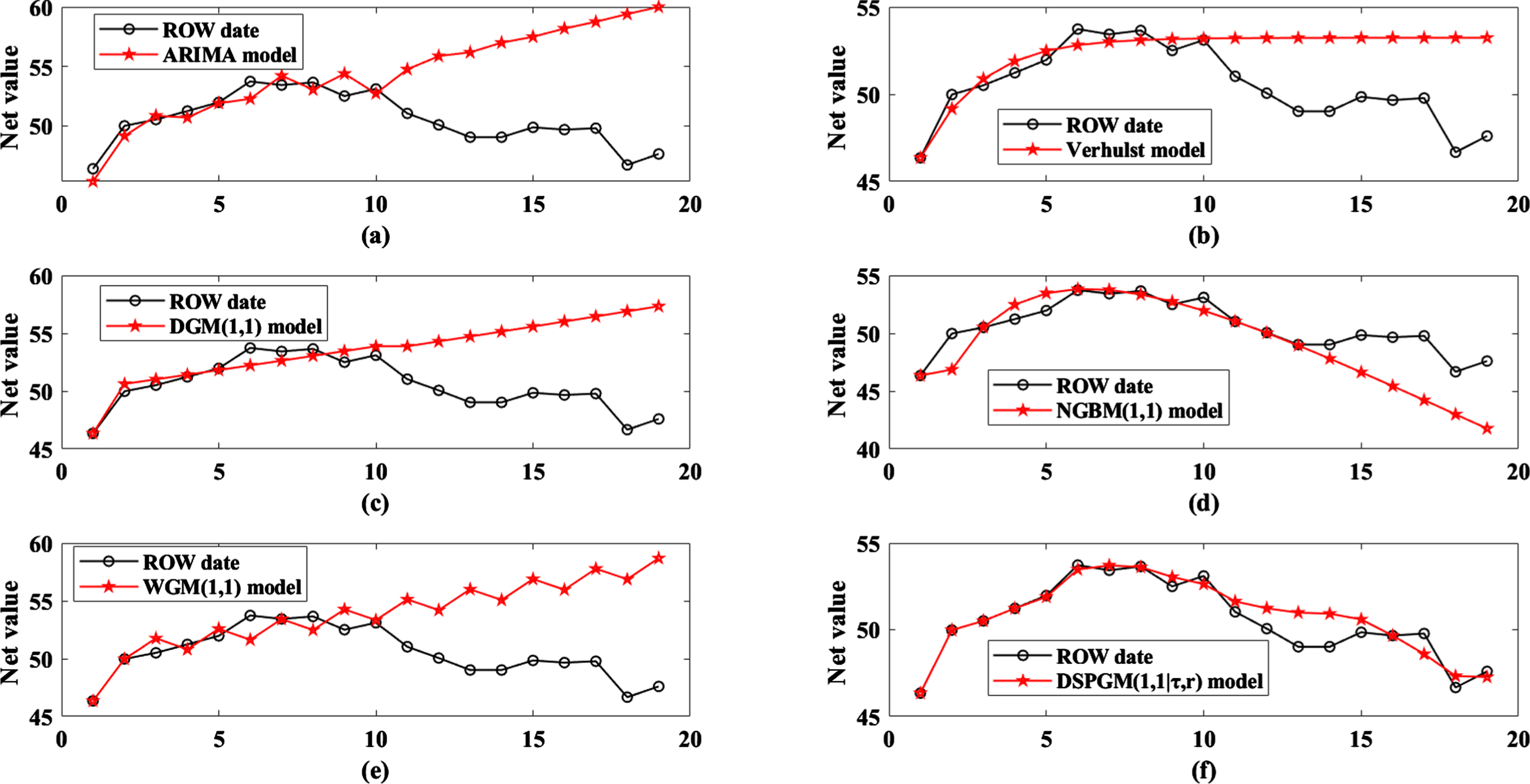
AIER Eye Hospital net change trend charts.

Then, look at the correlation coefficient between the results of each model and the real data. Table 6 and Fig. 9 show that in the ARIMA, traditional Verhulst, DGM(1,1), NGBM(1,1), WGM(1,1), and DSPGM(1,1|τ,r) models, the fitting results of the Shanghai composite index and the correlation coefficient R of the original data were 0.2133, 0.3550, 0.1709, 0.8642, 0.7351, and 0.9178, respectively. It can be seen that the correlation coefficient between the DSPGM(1,1|τ,r) model and the original data is much higher than the others. In summary, DSPGM(1,1|τ,r) is better than the ARIMA, traditional Verhulst, DGM(1,1), NGBM(1,1), and WGM(1,1) models in the forecasting of AIER Eye Hospital.

Fig. 9

Error comparison of each model on AIER Eye Hospital.

In the above four cases, the DSPGM(1,1|τ,r) model accurately predicts the net value change of the Shanghai Index, Kweichow Moutai, Shenzhen Index and AIER Eye Hospital. It can be found that the ARIMA, Verhulst, DGM(1,1), NGBM(1,1), and WGM(1,1) models often deviate from the true trend of the stock during stock forecasting, which show that the traditional grey model and some other non-grey models have great limitations in predicting the net worth of China’s stock market. The DSPGM(1,1|τ,r) model has already solved the problem of the traditional grey model not predicting the effect very well and solved the remainder of the models, which are complex and require considerable data, such as neural network and random forest models. Therefore, the proposal of the DSPGM(1,1|τ,r) model is of great significance to the prediction of China’s stock market.

6 Conclusion

In view of the phenomenon of the pulse of the stock market, this paper builds an impulsive differential equation and introduces the particle swarm optimization algorithm (PSO) to optimize the delay factor τ and nonlinear factor r. Based on this, the grey prediction model DSPGM(1,1|τ,r) with impulse delay of stock price is proposed. This paper describes its application in China’s Shanghai and Shenzhen Indexes market closing index prediction of the stock market and studied the Shanghai and Shenzhen stock closing price forecasts. The specific results are shown in Section 5. It can be concluded that the variation trend of the predicted results of the DSPGM(1,1|τ,r) model is basically the same as the real stock price.

In this paper, the impulse delay phenomenon of the stock market price system is combined with the modelling of the grey prediction model, and the grey model is proposed. This model has a good effect on stock price prediction research, so it has an important guiding role in the prediction of China’s stock market and is of great significance to both individual enterprises and the country. However, the delay time of the new model is the time delay intercepted from the original sequence and must be an integer. When the delay is of fractional order, further study is needed.

Footnotes

Acknowledgments

The authors are grateful to the editors and the reviewers for their insightful comments and suggestions. This work is supported by the Social Science Planning and Doctoral Program of Chongqing(2020BS58); Project of Humanities and Social Sciences Planning Fund of Ministry of Education of China (18YJA630022); Chongqing Natural Science Foundation of China (cstc2020jcyj-msxmX0649).

References

Rapach

and Zhou

, Forecasting Stock Returns, Handbook of Economic Forecasting 2 (2013), 328–383. dio: 10.1016/B978-0-444-53683-9.00006-2.

Paola

, Jonathan

, Werner

Werner K.

and Luis

, Fast and Adaptive Cointegration Based Model for Forecasting High Frequency Financial Time Series, Computational Economics 54(1) (2019), 99–112. dio: 10.1007/s10614-017-9691-7.

Rout

A.K.

, Dash

P.K.

, Dash

, et al., Forecasting financial time series using a low complexity recurrent neural network and evolutionary learning approach, Journal of King Saud University - Computer and Information Sciences 29(4) (2015), 536–552. dio: 10.1016/j.jksuci.2015.06.002.

Hyeuk

and Sang

T.H.

, The enhanced classification for the stock index prediction, Procedia Computer Science 91 (2016), 284–286. dio:10.1016/j.procs.2016.07.077.

Jigar

and Sahil

, Predicting stock market index using of machine learning techniques, Expert Systems with Applications 42 (2015), 2162–2172. dio: 10.1016/j.eswa.2014.10.031.

Paiva

F.D.

, Decision-making for financial trading: A fusion approach of machine learning and portfolio selection, Expert Systems with Applications 115 (2018), 635–655. dio: 10.1016/j.eswa.2018.08.003.

Jilani

T.A.

and Burney

S.M.A.

, M-factor high order fuzzy time series forecasting for road accident data: analysis and design of intelligent systems using soft computing techniques, Adv Soft Computer 41 (2007), 246–254. doi: 10.1007/978-3-540-72432-2_25.

Deng

J.L.

, Foundations of Grey Theory. Huazhong University of Science and Technology Press. 2002, in Chinese.

Duan

H.M.

, Xiao

X.P.

, Long

, et al., Tensor alternating least squares grey model and its application to short-term traffic flows, Applied Soft Computing Journal 89 (2020), 106145, doi: 10.1016/j.asoc.2020.106145.

10.

Wen

J.H.

, Wu

C.Z.

, Zhang

R.Y.

, et al., Rear-end collision warning of connected automated vehicles based on a novel stochastic local multivehicle optimal velocity model, Accident Analysis and Prevention 148 (2020), 105800. doi: 10.1016/j.aap.2020.105800.

11.

Duan

H.M.

and Pang

X.Y.

, A Multivariate Grey Prediction Model Based on Energy Logistic Equation and Its Application in Energy Prediction in China, Energy 229 (2021), 120716. doi: 10.1016/j.energy.2021.120716.

12.

Liu

, Wu

W.Z.

, Xie

W.L.

, et al., Application of a novel fractional grey prediction model with time power t erm to predict the electricity consumption of India and China, Chaos, Solitons and Fractals 141 (2020), 110429. doi: 10.1016/j.chaos.2020.110429.

13.

Zhao

H.Y.

and Wu

L.F.

, Forecasting the non-renewable energy consumption by an adjacent accumulation grey model, Journal of Cleaner Production (2020), 275. doi: 10.1016/j.jclepro. 2020.124113.

14.

Xiao

Q.Z.

, Shan

M.Y.

, Gao

M.Y.

, et al., Parameter optimization for nonlinear grey Bernoulli model on biomass energy consumption prediction, Applied Soft Computing (2020), 95. doi: 10. 1016/j.asoc.2020.106538.

15.

Xiao

Q.Z.

, Shan

M.Y.

, Gao

M.Y.

, et al., Evaluation of the coordination between China’s technology and economy using a grey multivariate coupling model, Technological and Economic Development of Economy, 2020, doi: 10.3846/tede.2020.13742

16.

, Wu

W.Q.

, Zhang

Y.Y.

, et al., Improved GM(1,1) model based on Simpson formula and its applications, Journal of Grey System 31(4) (2019), 33–46.

17.

Xie

N.M.

and Chen

N.L.

, The novel fractional discrete multivariate grey system problem with interval grey processing time, Applied Soft Computing 70 (2018), 513–524. doi: 10.1016/j.asoc.2018.06.004.

18.

Mao

S.H.

, Kang

Y.X.

, Zhang

Y.H.

, et al., Fractional grey model based on non-singular exponential kernel and its application in the prediction of electronic waste precious metal content, ISA Transactions 107 (2020), 12–26. doi: 10.1016/j.isatra.2020.07.023.

19.

Duan

H.M.

and Luo

X.L.

, A novel multivariable grey prediction model and its application in forecasting coal consumption, ISA transactions, 2021, 10.1016/j.isatra.2021.03.024.

20.

Wang

Z.X.

and Li

, Forecasting the monthly iron ore import of China using a model combining empirical mode decomposition, non-linear autoregressive neural network, and autoregressive integrated moving average, Applied Soft Computing Journal. 2020, doi: /10.1016/j.asoc.2020.106 475.

21.

Wang

Z.X.

and Hao

, An improved grey multivariable model for predicting industrial energy consumption in China, Applied Mathematical Modelling 40 (2016), 5745–5758. dio: 10.1016/j.apm.2016.01.012.

22.

Mao

S.H.

, Kang

Y.X.

, Zhang

Y.H.

23.

Zeng

and Li

, Improved multi-variable grey forecasting model with a dynamic background-value coefficient and its application, Computers & Industrial Engineering 118 (2018), 278–290. doi: 10.1016/j.cie.2018.02.042.

24.

Zeng

, Ma

and Shi

, A new-structure grey Verhulst model for China’s tight gas production forecasting, Applied Soft Computing (96) (2020), 106600, doi: 10.1155/2020/6514236

25.

, Liu

Z.B.

and Wang

, Application of a novel nonlinear multivariate grey Bernoulli model to predict the tourist income of China, Journal of Computational and Applied Mathematics 347 (2019), 84–94. doi: 10.1016/j.cam.2018.07.044.

26.

Liu

, Lao

T.F.

, Wu

W.Z.

, et al., Application of optimized fractional grey model-based variable background value to predict electricity consumption, Fractals-complex Geometry Patterns & Scaling in Nature & Society 2021, doi: 10.1142/S0218348X21500389

27.

Kayacan

, Ulutas

and Kaynak

, Grey system theory-based models in time series prediction, Expert Systems with Applications 37(2) (2010), 1784–1789. doi: 10.1016/j.eswa.2009.07.064.

28.

Duan

H.M.

, Xiao

X.P.

, Yang

J.W.

and Zeng

, Elliott wave theory and the Fibonacci sequence-gray model and their application in Chinese stock market, Journal of Intelligent and Fuzzy Systems 34(3) (2018), 1813–1825. doi: 10.3233/JIFS-17108.

29.

J.Z.

, Xu

and Gong

X.Z.

, The application of grey forecasting in stock price forecasting, Statistics and Decision-Making 1 (2007), 139–140. doi: 10.1631/jzus.2007.A1596.

30.

Wang

and Han

L.Y.

, The Application of Grey Model in the Prediction of China’s Stock Market, China Management Science 10 (2002), 287–290.

31.

Liu

, Guo

L.X.

and Xu

X.X.

, On the control stability of a three dimensional stock price system with time delays, Journal of Dynamics and Control 13(05) (2015), 382–387.

32.

Chen

X.Y.

and Dang

Y.G.

, Grey GM(1,1,t) model with time delay parameters and its application [J], Mathematics in Practice and Theory 45(04) (2015), 94–100.

33.

Huang

, Zhang

W.B.

, Zhao

, Peng

and Pu

, Forecast analysis of health human resources in Chongqing based on ARIMA model[J], China Rural Health Service Management 41(05) (2021), 326–331.

34.

Zhou

D.Q.

, The construction and parameter estimation method of grey Verhulst LS-SVM, Statistics and Decision 36(12) (2020), 59–63.

35.

Wang

, Huang

Z.Y.

, Zhang

Y.S.

and Wang

W.L.

, The application of indirect DGM(1,1) model in foundation pit settlement prediction, Geographical Spatial Information 16(05) (2018), 103–105+10.

36.

Chen

C.I.

, Chen

H.L.

and Chen

S.P.

, Forecasting of foreign exchange rates of Taiwan’s major trading partners by novel nonlinear Grey Bernoulli model NGBM(1, 1), Commun Nonlinear Sci Numer Simul 13 (2008), 1194–1204. doi: 10.1016/j.cnsns.2006.08.008.

37.

, Weighted cumulative generation and grey WGM(1,1,λ,t) model, Journal of Shandong Institute of Civil Engineering and Architecture 3 (2003), 76–78.

38.

Kennedy

and Eberhart

, Particle swarm optimization, Proceedings of ICNN’95 International Conference on Neural Networks 4 (1995), 1942–1948. doi: 10.1109/ICNN. 1995.488968.

39.

Chang

, Characteristics of my country’s Stock Price Volatility and Government Macro Control, Price Theory and Practice 5 (2016), 21–22.