Unsupervised labelling of remote sensing images based on force field clustering

Abstract

Remote sensing image segmentation provides technical support for decision making in many areas of environmental resource management. But, the quality of the remote sensing images obtained from different channels can vary considerably, and manually labeling a mass amount of image data is too expensive and inefficiently. In this paper, we propose a point density force field clustering (PDFC) process. According to the spectral information from different ground objects, remote sensing superpixel points are divided into core and edge data points. The differences in the densities of core data points are used to form the local peak. The center of the initial cluster can be determined by the weighted density and position of the local peak. An iterative nebular clustering process is used to obtain the result, and a proposed new objective function is used to optimize the model parameters automatically to obtain the global optimal clustering solution. The proposed algorithm can cluster the area of different ground objects in remote sensing images automatically, and these categories are then labeled by humans simply.

Keywords

Remote sensing core data nebular clustering parameter optimization objective function

1 Introduction

Remote sensing image clustering analysis is aimed at high-spectral annotation to provide technical support for decision-making in fields such as water resource evaluation, large-scale engineering site selection, geological environment monitoring and evaluation, evaluation of changes in arable land and deforestation, vegetation change research, and seasonal pasture change analysis. Due to the different geological and weather conditions, remote sensing images vary considerably, it is costly and difficult to obtain the labeled data for training. So many unsupervised techniques have been gradually developed and applied to label the massive remote sensing image samples. It can save a lot of human resources and overcome subjective factors of human labeled partly.

Clustering methods for remote sensing images can be divided into mean-shifting, density-based, hierarchical [1], spectral [2, 3], grid-based [4] methods, and so on. In recent years, there are many new research directions of the clustering algorithm. Various improved graph clustering, spectral clustering, and multi-scale clustering methods have been proposed. Both graph clustering and spectral clustering are algorithms evolved from graph theory, which have been widely used in clustering. Multi-scale clustering uses more than two indicators to measure the relationship between data and cluster the data. In addition, deep clustering is also the latest research direction. Compared with traditional methods, these new clustering methods have achieved good results in different application scenarios. These methods can solve remote sensing image clustering to some extent, however, there are still exist some disadvantages: First, no matter the image pixel points are decomposed in any way such as RGB, HSV or Lab, the pixel points show irregular distribution, as shown in Fig. 2(c). Visually, the distribution density of pixels is not uniform, and there is no obvious boundary between clusters of different types, and no obvious spherical cluster is formed. Using the centralization method to cluster the image will result in the wrong clustering of the aspheric surface cluster and lead to the defect of clustering effect. The dense-based method will cause the bad clustering of the sphere clusters with uneven density distribution to some extent, and still cannot achieve better clustering effect. The two types of methods can not take into account the clustering problem of arbitrary shape clusters, and the combination of Euclidean distance and domain density can avoid wrong clustering to a certain extent, which is helpful to solve the problem that can not be solved by using the above scale clustering alone, that is, it can reduce the sensitivity of distance-based clustering method to point distance, It can also avoid clustering errors caused by uneven density.

Next, existing clustering algorithms often require humans to determine some hyperparameters, such as the number of clusters, the measurement of point density, etc., and manually assisted determination is required no matter using the elbow method, Average Silhouette coefficient and the square error in the cluster.

So, the clustering segmentation problem of remote sensing images cannot be easily addressed using existing algorithms unsupervised. To find a suitable unsupervised clustering method for different shapes and density distributions, we propose the PDFC, and a brief description of this approach follows: the number of clusters can be confirmed by the peaks in the core data point distribution, and the positions of the cluster centers and the point density weights are also determined by the peaks. In the process of clustering, to avoid the disadvantage of using distance as the single index of clustering, we introduce the neighborhood density and Euclidean distances (hereinafter referred to simply as distance) between points as the index of clustering, and take the density weight error and the distance error of the center of mass as the convergence condition to complete the iterative process. Meanwhile, setting up a reasonable double objective optimization process to get the global optimal clustering results achieves a better clustering effect.

Contributions:

Based on the discrete distribution characteristics of pixel points, a computing process of a neighboring point set with low time complexity was designed to control the algorithm complexity within O (nlog (n)).

Our algorithm solves the problem of the number of sample clusters and the selection of an initial clustering center point in the case of no supervision and no prior. This avoids convergence to the local optimum caused by the improper selection of an initial clustering center and accelerates the convergence process of the approach.

Inspired by nebula formation, the iterative process of the clustering approach uses density weight and distance as basis of data point clustering. It avoids the clustering center offset due to outliers, making it especially suitable for the local uneven densities of aspheric clustering like remote sensing image.

The screening of the optimal clustering results is set as a double objective optimization process, and the optimal clustering result is obtained by setting the double objective equilibrium optimization function of the average point density and the silhouette coefficient (SC) to avoid the situation of the single objective optimization falling into a local optimal solution.

2 Related work

Many clustering algorithms can be used for remote sensing image clustering. In the following, we discuss the advantages and disadvantages of various clustering algorithms to compare them with PDFC. Centroid-based algorithms such as Kmeans [5], K-medoid [6], and other improved methods [7 –9] have the advantages of simple principles, convenient implementation, and fast convergence. However, because the iterative process tends to fall into the local optimal solution, the clustering effect is flawed. In response to this problem, Fritzke [10] allowed a few and limited retries for the recent jump. the improved algorithm solved the problem of the Kmeans (Kmeans-u*) iteration process ending prematurely due to local minimization, which improved the clustering performance of the Kmeans algorithm to some extent. In contrast, this type of algorithm only uses distance as the clustering scale, and such an effect is not suitable for aspheric clusters.

Fuzzy c-means (FCM) and other improved methods [7 , 11–13] calculate each element in the membership matrix to represent the degree of the sample belonging to a certain category. They use the Lagrange multiplier method to calculate the minimum value of the function to complete the clustering process. However, selecting the location of the initial center of mass and the number of centers of mass is always unavoidable in soft clustering algorithms. Therefore, Pei et al. [14] proposed a novel density-based FCM algorithm (D-FCM) by introducing density of the point distribution into each sample. The density peak was used to some extent to determine the number of clusters and the initial membership matrix.

Meanwhile, the Gaussian mixture model (GMM) [15, 16] clustering algorithm is equivalent to the generalization of Kmeans and other algorithms. The characteristics of the data can be better described with only few parameters. Neagoe et al. [17] proposed a new method for semi-supervised clustering of remote sensing images using a (GMM-EM) clustering cascade according to the difficulties in remote sensing image clustering; they selected the number of clustering pixels to be added to the training set according to the GMM capabilities for remote sensing image clustering. However, the GMM algorithm incurs a large computational cost and demonstrates slow convergence.

The density-based clustering algorithm represented by DBSCAN [18] shows strong robustness for uniform-density clusters of any shape and can divide clusters well, but it is not easy to select a suitable density threshold, especially for clusters with a large difference in density. The circular radius needs to be adjusted constantly to adapt to different cluster densities, and no reference has been established. Furthermore, DBSCAN requires neighborhood queries for all objects and the propagation of labels from one object to another. This scheme is time-consuming and thus limits its applicability for large datasets. Li and He et al. [19, 20] used the improved DBSCAN method combined with supervised learning for remote sensing image clustering to detect ships and vehicles. Mai [21] proposed anytime parallel density-based clustering (AnyDBC) to compress the data into smaller density-connected subsets called primitive clusters and labeled objects based on the connected components of these primitive clusters to reduce the label propagation time. This improved approach showed a reduced range query and label propagation time compared to DBSCAN.

More and more scholars use the combination of clustering and neural network [22], and apply it to remote sensing image recognition. This method has high accuracy, but it requires high computing resources. Recently, Chen et al. [23] proposed a ReDO model to achieve a certain degree of unsupervised image segmentation by using the method of deep clustering. Gargees et al. [24] proposed a deep feature clustering for remote sensing imagery land cover analysis. These approaches are especially suitable for datasets with large image data and can complete tasks such as semantic segmentation. However, due to the need to manually specify the number of clustering and other supervisory operations, completely unsupervised clustering cannot be achieved.

3 Point density force field clustering process

Different geological environments present a certain area distribution in remote sensing images. If each pixel is analyzed one by one, unnecessarily high computing resources will be consumed. In this study, the simple linear iterative cluster algorithm (SLIC) [25 –27] is adopted as a preprocessing image clustering step (In other clustering algorithms for comparison, SLIC is also used as the preprocessing step before clustering).

The SLIC algorithm uses the super-pixel to represent the pixel value of a small area, which has two advantages: firstly, for remote sensing image, clustering each pixel one by one will bring a huge amount of computation, which is neither economical nor necessary; secondly, SLIC algorithm is equivalent to the smooth denoising process of the image, which eliminates the influence of high-frequency noise points in the image on the clustering effect.

3.1 Core data weight density distribution

The distribution of superpixel data points is in a chaotic state, we can extract certain key samples from the data points based on a statistical concept and infer the correctness and appropriateness of the clustering result according to the differences in the densities of the key samples. That can eliminate the interference in inessential samples and strengthen the links between key samples. Because the preprocessed image data of the three channels of RGB are all discrete values between 0 and 255, any data point with a large gap in the RGB channel value cannot be a neighboring point. Therefore, it is meaningless to calculate the distance between large-gap data points. First, we use quicksort [28] to sort and store the superpixel values of the RGB three channels separately and set the step length as s. The R channel pixel value of the data point x_i is r_i, and the R channel pixel value of the data point x_j is r_j. When calculating the distance d_ij between data point x_j and data point x_i (with x_j meeting the range condition r_j ∈ [r_i - s, r_i + s], and the constraint condition r_i - s ≥ 0, r_i + s ≤ 255), if $d_{ij} \leq d_{R} = \sqrt{3 \cdot s^{2}}$ , data point x_j belongs to the neighboring point collection $R_{i}^{'}$ of point x_i set by the R channel. The above steps are repeated to calculate the neighboring point collections $G_{i}^{'}$ and $B_{i}^{'}$ set by the G and B channels, respectively. Then, we obtain the neighboring point collection N_i (x_i) in the range of the step-length size s. The calculation process of neighboring points is shown in Fig. 1. $N_{i} (x_{i}) = R_{i}^{'} \cup G_{i}^{'} \cup B_{i}^{'}$ (1) The point density threshold is set as $m = \sum_{i = 1}^{n} \frac{N_{i} (x_{i})}{n}$ , where n is the number of core points.

E_i is an edge point and C_i is a core point. The distinction between E_i and C_i is determined by the following equation: $x_{i} \in {\begin{matrix} E_{i}, N_{i} (x_{i}) ⩽ m \\ C_{i}, N_{i} (x_{i}) > m \end{matrix}$ (2)

The number of neighborhood points is used as the weight of the core point. We calculate all core points weight, and the discrete distribution of the density weights of core points in the three-dimensional RGB space (hereinafter referred to as density distribution) is obtained. Special instructions: as the RGB channel is a three-dimensional space, the display effect is not easy to show. Therefore, the images in this paper are all replaced by R and G two-channel matrix images. It can be seen from Fig. 2(b) that the distribution of the superpixel data points presents an irregular shape, no definite clustering center, uneven densities of data points, and no obvious hierarchy. In the remote sensing superpixel scatter diagrams shown in Fig. 2(c), the red points are the edge points and the green points are the core points with the step length s equal to 3.

3.2 Peak points converge to select an initial center of mass

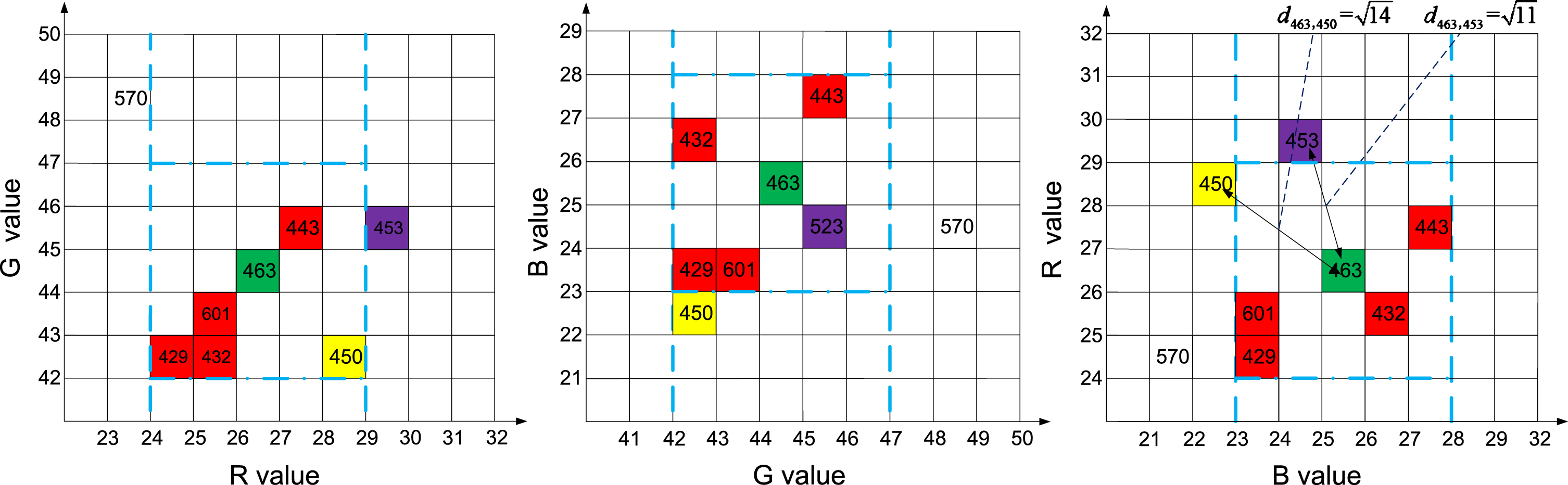
To determine the RGB coordinates of the peak points, it is necessary to filter the density distribution first so that it presents an approximately continuous state in the RGB space. In this study, a multidimensional Gaussian kernel function is adopted to complete this process. The expression of this kernel function is as follows: $p (x; μ, Σ) = \frac{1}{(2 π)^{D / 2} | Σ |^{1 / 2}} exp (- \frac{1}{2} (x - μ)^{T} Σ^{- 1} (x - μ)$ (3) where μ = E (x), Σ = Cov (x) = E [(x - μ) (x - μ) ^T] Here, μ is the mean vector, Σ represents the covariance matrix D represents the dimension of the current Gaussian kernel function. $μ = [\begin{matrix} μ_{1} \\ μ_{2} \\ ⋮ \\ μ_{D} \end{matrix}]$ (4) $Σ = [\begin{matrix} Σ_{11} & Σ_{12} & \dots & Σ_{1 D} \\ Σ_{21} & Σ_{22} & \dots & Σ_{2 D} \\ ⋮ & ⋮ & ⋱ & ⋮ \\ Σ_{D 1} & Σ_{D 2} & \dots & Σ_{DD} \end{matrix}]$ (5)

Fig. 1

RGB space neighborhood range for point 463 with a step-length size of 2. The above figure shows the neighborhood range of point 463, where the step-length size s is 2, the cut-off distance d_R is $\sqrt{12}$ , the set of $R_{463}^{'}$ determined by the R channel is (429, 601, 432, 443), the set of $G_{463}^{'}$ is (429,601,432,443,453), and the set of $B_{463}^{'}$ is (429, 601, 432, 443, 453). The yellow data point 450 satisfies the constraint conditions in both channel R and channel G; however, because its distance from point 463 is $\sqrt{14}$ , it is outside the neighborhood range of point 463. The purple data point 453 does not meet the constraint condition in channel R, but because it is $\sqrt{11}$ away from point 463, the neighborhood range of point 463 is (429, 601, 432, 443, 453). The blue dotted line indicates the range of neighboring pixel values that are expected to be detected by each channel). The core point is taken as the main research object, and the neighboring point density N_i (x_i) is taken as the weight of data point x_i.

Fig. 2

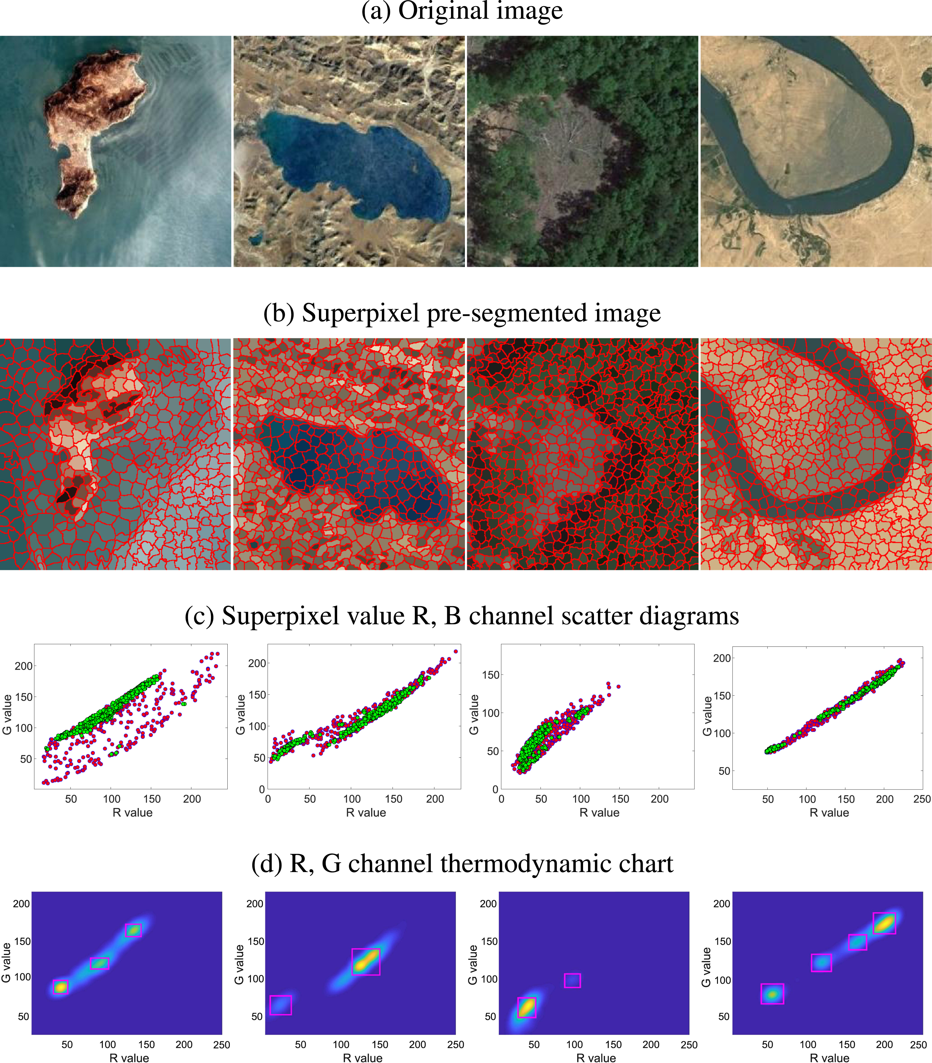
Scatter image after superpixel segmentation and the density heat map. (a) are the original image, (b) are the image pre-processed by SLIC super-pixel segmentation, (c) are the distribution of super-pixel points in G-R space, green represents the core points, red represents the edge points, (d) are the thermal distribution of filtered super-pixel scattered points, and red box is the detected peak points.

Since the point density is distributed in the RGB three-space, both the density distribution and the Gaussian kernel function are three-dimensional and D is equal to 3. The three dimensions of the kernel function RGB are set as uncorrelated, and the size of the kernel function is set as a random natural number between 4 and 10. The filtered thermodynamic density distribution can be obtained. The density heat map after Gaussian filtering is shown in Fig. 2(d). There are several peak regions in the thermodynamic chart of the density distribution, and these are the high-density points where superpixel values gather. We use the maximum value in the 26 connected regions of the spatial search neighboring data points to find several peak points in the three-dimensional heat map. With a change in the step-length size s, the neighborhood density of core points also changes. Therefore, the location and number of thermal map peaks will vary. By detecting the peak in the density distribution, the initial clustering center of the distribution of superpixel data points can be determined. The RGB coordinates and point density weights of the detected peak points are taken as the coordinates and weights of the initial centroid of the clustering iteration process, respectively.

3.3 Nebular clustering iterative process

We make a simple analogy, and liken the PDFC to the nebula formation process. The less massive planets orbit the more massive stars. Massive fixed stars are first formed, followed by planets, which eventually leads to the development of stable nebulas.

First, several concepts need to be defined in this section:

1.The peak point is defined as a fixed star.

2.The other core data points are defined as planets.

3.edge points are satellites.

4.A peak point and core points of the same cluster as the peak form a nebula.

5.The average point density of all core points in a nebula is defined as the gravitational value of the nebula.

To simplify the clustering process, We ignore the gravity of satellites and the gravity between planets and only consider the gravity between fixed stars and planets. Only the magnitude of this gravitational force, and not its direction, is considered. The mass of a nebula is an important index of its gravitational range. In the clustering process, the greater the point density, the wider the gravitational range. During this process, peak point P_i are thought of as fixed stars, and the nebula formed from it is set as z_i. The other core data points are thought of as planet points c_j, the density of the nebula $\bar{ρ_{z_{i}}}$ is defined as the mean density weight of all core points C belonging to the cluster.

Step1: The density of a planet c_j is ρ_{c
_j}, the density of the nebula z_i is $\bar{ρ_{z_{i}}}$ , and The distance between the planet and the fixed star is d_ij. So, the gravitational force between them is as follows: $F_{ij} = \frac{ρ_{c_{j}} \times \bar{ρ_{z_{i}}}}{d_{ij}^{2}}$ (6) The gravitational force between all planetary points and the stellar point is calculated. The planetary point and the stellar point with the largest gravitational force values are clustered into a cluster to form the nebula of the star and complete an iteration.

Step2: The coordinates of the mean positions of all the planets in the nebula are used as the new fixed star positions, and the average density value of the planet belong the nebula is calculated as the density value of the new fixed star. Step1 and Step2 are repeated. The core points of the nebula are constantly adjusted and until the position of the fixed stars and the density value of the nebula remain essentially unchanged, i.e., the approach converges. The iteration is then stopped to obtain the clustering results of all star and planet points. Finally, the satellite points and the nearest planet point are clustered into one cluster to complete the clustering process. The gravitational map of stellar planetary points is shown in Fig. 3.

3.4 Time complexity assessment

If an image has n superpixels, and when calculating the distance from each data point to all the other data points, we should have to do n × n calculations, and the time complexity is O (n²). The time cost is extremely high. The time complexity of Sections 3.1 is O (n (log (n))). The time complexity of performing in Sections 3.2 and 3.3 is O (n), because it is only necessary to traverse all the superpixel points a constant number of times. Thus, the overall time complexity of the PDFC approach is O (n (log (n))). It is also competent in the direct processing of pixel-level images. That is to say, even without SLIC pretreatment, PDFC can also directly complete the task of image clustering on a regular computer.

Fig. 3

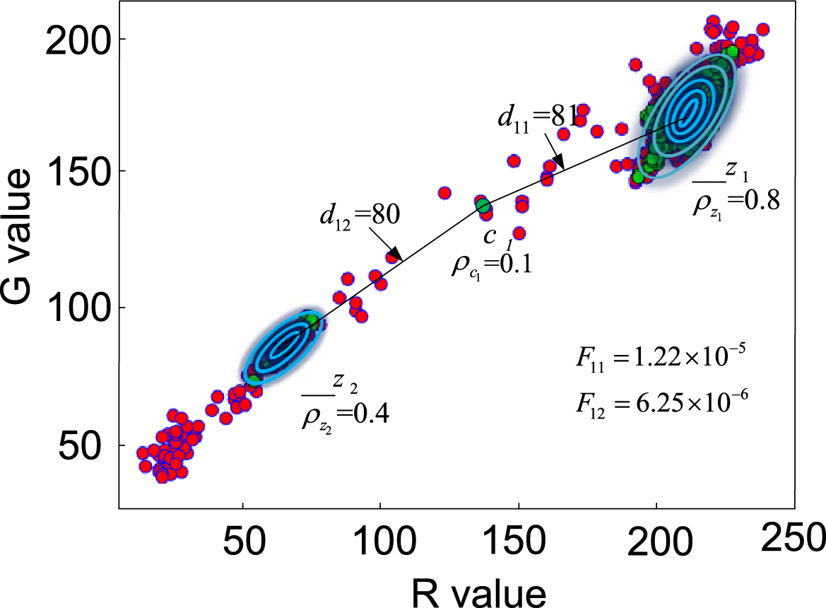
Gravitational map of stellar planetary points.

The distance between planet point e₁ and two fixed star points is 80 and 81, and z₂ is closer. However, the gravitational values are 1.22 × 10^-5 and 6.25 × 10^-6. Then, e₁ is more easily attracted to z₁. So e₁ should be classified as z₁ in this iteration.

Algorithm 1

General framework of the nebular clustering iterative process
Require: Density weights and RGB space position coordinates of all fixed star and planet points under the current step-length size.
Ensure: The fitness values of the initial population are calculated.
Repeat:
1: Calculate the gravitational value F_ij between all the planet points and the star points;
2: Gather the planet and fixed star points with the greatest gravitational value F_ij into one category;
3: Recalculate the mean coordinate and density of each cluster of stars as the location and density of the new nebula.
Until: The position of the fixed stars and the mean density of the nebulae tend to remain the same.

4 Objective function

Although the number of clusters, boundary distance, and other parameters can be set manually, without sufficient prior knowledge and multiple tuning attempts, it is difficult to find suitable evaluation criteria for these clustering parameters. As the distribution of the remote sensing image density is uneven, the clustering center is not obvious, and using a single objective optimization can easily lead to deviations from the global optimal solution. To avoid the disadvantages of single objective function optimization, we set the entire clustering process as a double objective optimization process, and an optimal clustering result is obtained by setting the double objective equilibrium optimization function of the standard deviation of the average point density and the SC. In terms of the distance, we expect a larger total SC to provide better clustering results. The equation to determine SC is as follows: $SC (i) = \frac{b (i) - a (i)}{max {a (i), b (i)}}$ (7) Where a (i) is the average distance between classification vector i and all other points in the cluster to which it belongs, and b (i) is the average distance between classification vector i and all other points in the cluster nearest to it.

Fig. 4

Iterative convergence curve and objective function curve of the four images. (a) and (b) are the graphs of distance and weight error convergence. (c) are different step-lengths correspond to the value of the objective function J

Table 1

Summary of notations

Notations	Explanation
d _ij	The distance between data point x_j and data point x_i
s	Step-length size
x _i	The i-th data point
x _j	The j-th data point
r _i	The R channel pixel value of the data point x_i
r _j	The R channel pixel value of the data point x_j
D _R	Cut-off distance
$R_{i}^{'}$	Neighboring point collection of point x_i set by the R channel
$G_{i}^{'}$	Neighboring point collection of point x_i set by the G channel
$B_{i}^{'}$	Neighboring point collection of point x_i set by the B channel
N_i (x_i)	The weight of data point x_i (The number of the neighboring collection points)
m	The point density threshold
E _i	The edge points (thought of as satellite)
C _i	The core points (thought of as planet points)
P _i	The peak points (thought of as fixed star points)
z _i	The nebula formed from the fixed star
$\bar{ρ_{z_{i}}}$	The density of the nebula z_i
c _j	The planet point
ρ_{c _j}	The density of a planet point
F _ij	The gravitational force between the nebula and the planet point
a (i)	The the average distance between classification vector i
b (i)	The the average distance between classification vector i and all other points in the cluster nearest to it
SC (i)	The silhouette coefficient (SC)
J	The objective function
$\bar{μ_{i}}$	The mean of the density weight of the i-th cluster point
ρ_j	The density weight of the j-th point
n _i	The number of data points for the i-th cluster
k	The number of clusters
n	The number of data points in the sample set
map (r_i)	Indicator function
δ	The number of data points in the sample set
Σ	The covariance matrix
NMI	The Normalized Mutual Information
RI	The Rand Index
ARI	The Adjust Rand Index
JC	The Jacarrd Index

Fig. 5

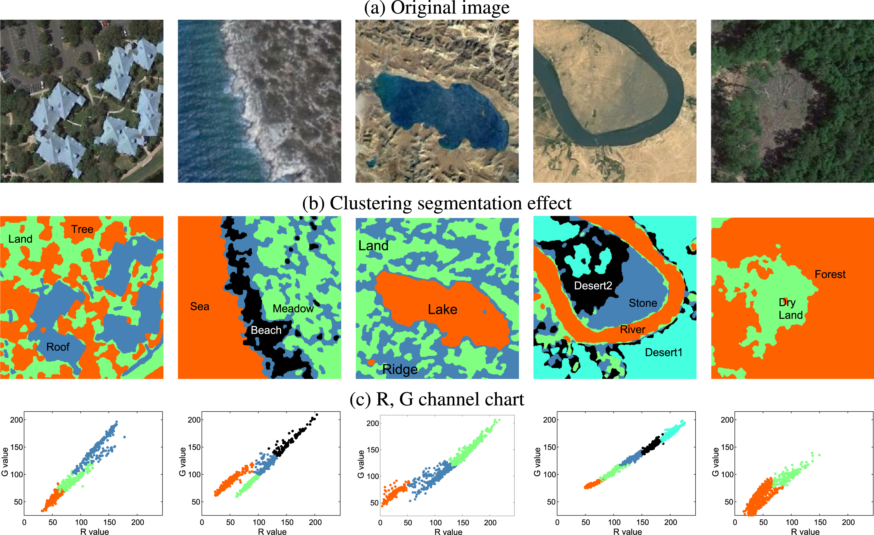
The clustering segmentation effect display of PDFC on the tag-free UCMerced-LandUse remote sensing dataset.

In terms of the point density, the mean value of the density weight standard deviation of all clusters that contain points should be obtained. We expect that the clustering result reduces the point density deviation of the data points of the same category of ground objects to the maximum extent possible, such that the data point density of the same category of ground objects is similar. Therefore, the objective function can be set as the ratio of the mean standard deviation of the point density weight within the cluster to the mean of the SC. When the smaller the objective function value is, the better the clustering effect is. Therefore, the optimization process can be completed by comparing the clustering results of different step parameters.

Objective function J can be expressed as follows: $J = \frac{\frac{1}{k} \sum_{i = 1}^{k} \sqrt{\frac{1}{n_{i}} \sum_{j = 1}^{n_{i}} {(ρ_{j} - \bar{μ_{i}})}^{2}}}{\frac{1}{n} \sum_{i = 1}^{n} SC (i)}$ (8) Here, ρ_j is the density weight of the j-th point, and $\bar{μ_{i}}$ is the mean of the density weight of the i-th classification cluster point; SC (i) is the SC of the i-th point; n_i is the number of data points for the i-th cluster; k is the number of clusters, and n is the number of data points in the sample set. As can be seen from Fig. 4(a), (b), the error in the iteration can converge to almost 0 after more than ten iterations. The minimum J value corresponds to the optimal clustering result are shown in Fig. 4(c), and the default value here means that the entire image is clustered into one cluster, and the target function is NAN.

5 Experiment

In this study, the dataset image was first preprocessed by the SLIC superpixel segmentation algorithm to produce a collection of superpixels for each image. PDFC verifies with the other five clustering algorithms on the super-pixel dataset rather than the original image dataset.

5.1 Index

This paper compares the following indicators of different algorithms: Accuracy, Normalized Mutual Information (NMI), Rand index (RI), Adjusted Rand Index (ARI), Jacarrd Index (JI). The symbol used for the index does not conflict with the symbol representation above and it is not listed in Table 1.

5.1.1 Accuracy

The formula for calculating the Accuracy of sub-datasets is as follows: $Accuracy = \frac{\sum_{i = 1}^{n} δ (s_{i}, map (r_{i}))}{n}$ (9) Where r_i and s_i represent the obtained label and the real label corresponding to data point x_i, respectively; n represents the total number of data points, and δ represents the indicator function, as follows: $δ (x, y) = {\begin{matrix} 1 & if x = y \\ 0 & otherwise \end{matrix}$ (10) The map in the equation represents the optimal cluster object re-allocation, to ensure correct statistics.

5.1.2 Normalized Mutual Information

The formula derivation of Normalized Mutual Information (NMI) is given below: Suppose the joint distribution of two random variables (x, y) is P (i, j). The marginal distributions are P (i) and P′ (j). I (x ; y) is the mutual information. It is the relative entropy of the joint distribution P (i, j) and the product distribution P (i) (j); the formula is as follows: $I (x, y) = \sum_{i = 1}^{| x |} \sum_{j = 1}^{| y |} P (i, j) log (\frac{P (i, j)}{P (i) P^{'} (j)})$ (11) The joint probability distribution $P (i, j) = \frac{| x_{i} ⋂ y_{j} |}{N}$ in the above formula: $NMI (x, y) = \frac{2 I (x, y)}{H (x) + H (y)}$ (12)

$H (x) = - \sum_{i = 1}^{| x |} P (i) log (P (i)); H (y) = - \sum_{j = 1}^{| y |} P^{'} (j) log (P^{'} (j))$ (13) The probability function in the denominator P (i) = x_i/N. P (i) is the probability distribution function of i and P′ (j) is the probability distribution function of j.

5.1.3 Rand Index, Adjust Rand Index and Jacarrd Index

Let the clustering result of be C ={ C₁, C₂, ⋯ , C_m }, and the known partition is P ={ P₁, P₂, ⋯ , P_m }, Rand Index (RI) [29] and Jacarrd Index (JI) [29], the formula is as follows: $RI = \frac{a + d}{a + b + c + d}$ (14) $JI = \frac{a}{a + b + c}$ (15) Where, a means that the two data objects belong to the same cluster in C and the same group in P; b means that the two points belong to a cluster in C, but belong to different groups in P. c means that the two points do not belong to the same cluster in C, while P belongs to the same group of d means that the two points do not belong to the same cluster in C and are in different groups in P. The higher the evaluation value of these two indexes is, the closer the clustering result is to the real partition result, the better the clustering effect is.

The Adjust Rand Index (ARI) assuming that the distribution of the model is random, that is, the division of P and C is random, then the number of data points of each category and each cluster is fixed.

$ARI = \frac{RI - E (RI)}{max (RI) - E (RI)}$ (16)

E (RI) is the mean value of each cluster RI, and max(RI) is the maximum value of each cluster RI.

Accuracy is a simple and transparent evaluation measure. NMI can be information-theoretically interpreted. The RI and ARI penalize both false positive and false negative decisions during clustering. The F measure in addition supports differential weighting of these two types of errors. These five indexes can be used to evaluate the clustering effect of various algorithms.

5.2 Experiment

5.2.1 Experiment I

The ‘2015 high-resolution remote sensing image of a city in southern China’ dataset [30] of the CCF Big Data competition was used as the dataset for verifying the algorithm clustering effect. It included 10,000 original geological remote sensing images and ground-truth images with a size of 256 × 256 pixels. Since all images of the dataset are not divided, in order to better verify the clustering discrimination of the five algorithms. We extracted 5000 remote sensing images with different ground object types for the validation dataset and divided them into 20 sub-datasets with 250 sample images each. In Fig. 6, compared with other algorithms, the mean accuracy of the PDFC approach for this dataset is in a higher range and the boxes are smaller.

Fig. 6

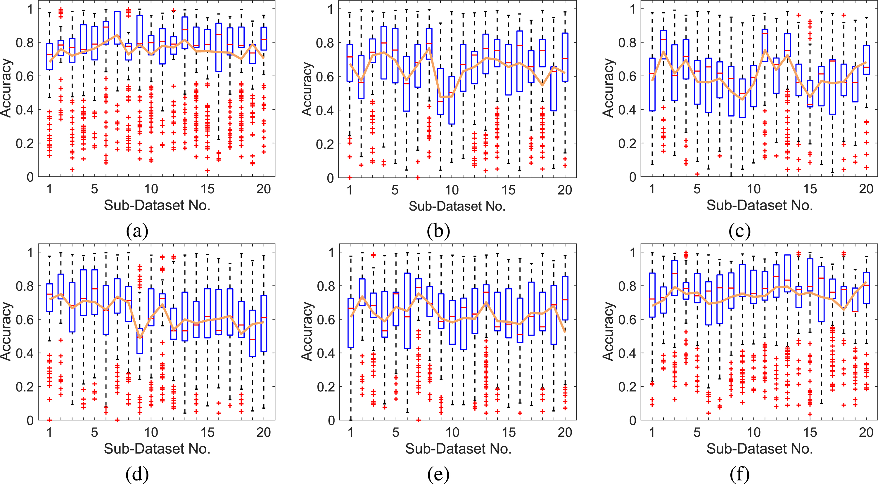
Box graphs of the accuracy of different clustering algorithms: (a) PDFC (b) AnyDBC (c) D-FCM (d) Kmeans-u* (e) GMM-EM and (f) ReDO. The orange line in the graphs represents the mean value of ACC, the blue box represents the centralized distribution of ACC, the red line of box type represents the median and the plus sign represents the outlier point.

Table 2

Comparison of mean values for various algorithms on four indices on dataset, and the bold is the maximum

Index	Algorithm	Ten subdatasets
		1	2	3	4	5	6	7	8	9	10
NMI	PDFC	0.834	0.857	0.921	0.802	0.875	0.846	0.826	0.895	0.791	0.829
	GMM-EM	0.806	0.764	0.868	0.855	0.784	0.856	0.765	0.773	0.751	0.841
	AnyDBC	0.746	0.827	0.797	0.586	0.645	0.538	0.762	0.752	0.787	0.791
	D-FCM	0.724	0.713	0.747	0.489	0.788	0.789	0.565	0.642	0.673	0.677
	Kmeans-u*	0.684	0.607	0.753	0.876	0.657	0.798	0.681	0.748	0.704	0.731
	ReDO	0.817	0.915	0.941	0.795	0.625	0.889	0.815	0.708	0.869	0.765
RI	PDFC	0.842	0.857	0.774	0.777	0.827	0.904	0.853	0.665	0.894	0.805
	GMM-EM	0.742	0.852	0.805	0.795	0.529	0.569	0.694	0.552	0.783	0.671
	AnyDBC	0.661	0.613	0.714	0.544	0.614	0.819	0.634	0.599	0.758	0.453
	D-FCM	0.554	0.903	0.582	0.514	0.694	0.852	0.581	0.679	0.646	0.505
	Kmeans-u*	0.724	0.764	0.599	0.797	0.501	0.788	0.872	0.527	0.673	0.795
	ReDO	0.817	0.875	0.879	0.805	0.81	0.869	0.815	0.508	0.835	0.765
ARI	PDFC	0.728	0.871	0.801	0.796	0.828	0.855	0.873	0.892	0.964	0.825
	GMM-EM	0.714	0.743	0.797	0.716	0.796	0.725	0.808	0.622	0.763	0.505
	AnyDBC	0.494	0.869	0.603	0.713	0.628	0.653	0.637	0.583	0.694	0.661
	D-FCM	0.463	0.825	0.823	0.684	0.815	0.675	0.514	0.672	0.811	0.776
	Kmeans-u*	0.666	0.793	0.673	0.507	0.684	0.808	0.802	0.774	0.802	0.711
	ReDO	0.812	0.748	0.857	0.765	0.852	0.799	0.815	0.848	0.927	0.765
JC	PDFC	0.851	0.742	0.794	0.622	0.651	0.884	0.848	0.621	0.856	0.793
	GMM-EM	0.756	0.636	0.519	0.532	0.733	0.593	0.749	0.646	0.691	0.516
	AnyDBC	0.505	0.412	0.404	0.321	0.423	0.631	0.684	0.511	0.798	0.362
	D-FCM	0.415	0.691	0.288	0.291	0.314	0.663	0.758	0.579	0.526	0.303
	Kmeans-u*	0.513	0.532	0.341	0.656	0.47	0.794	0.657	0.417	0.496	0.463
	ReDO	0.827	0.736	0.815	0.595	0.515	0.879	0.757	0.557	0.807	0.765

The mean values of the NMI, ARI, RI, and JC of the sub-datasets were calculated to test the performance of the algorithms. The closer the four indicators are to 1, the better the clustering effect will be. Due to the limited space, we randomly select 10 sub-datasets for presentation in Table 2, from which it can be seen that PDFC has achieved a large value on most of the molecular datasets, representing a good clustering effect.

Fig. 7

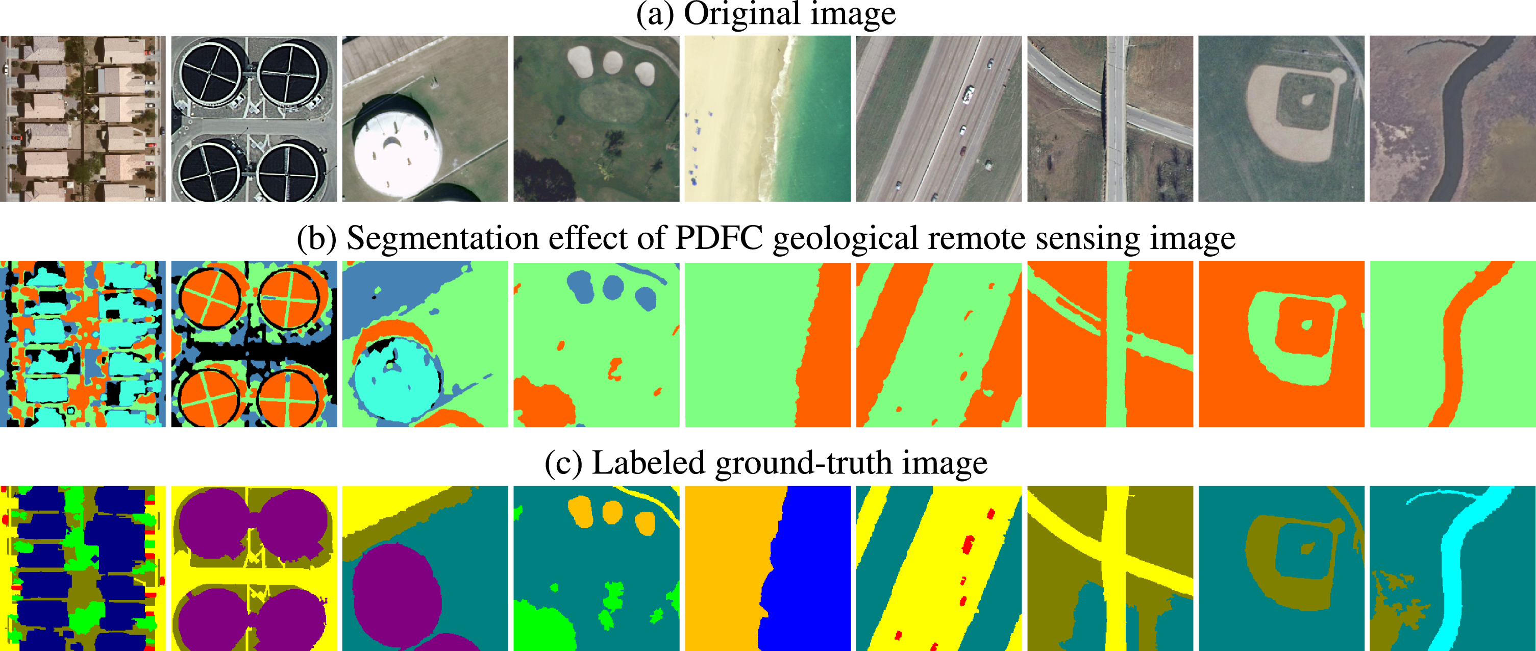
The clustering segmentation effect of PDFC on the ‘2015 high-resolution remote sensing image of a city in southern China’ dataset

Fig. 8

The clustering segmentation effect of PDFC on the ‘UCMerced-LandUse’ remote sensing dataset

Table 3

Exponential performance of various methods on ’UCMerced-LandUse’ dataset

Index	Acc	NMI	ARI	RI	JI
PDFC	0.871±0.075*	0.913±0.031*	0.867±0.124*	0.927±0.052*	0.846±0.102*
D-FCM	0.795±0.125	0.852±0.172	0.724±0.201	0.835±0.105	0.805±0.172
Kmeans-u*	0.810±0.010	0.825±0.127	0.781±0.195	0.816±0.083	0.735±0.134
AnyDBC	0.641±0.312	0.712±0.079	0.532±0.183	0.751±0.182	0.593±0.157
GMM-EM	0.791±0.143	0.813±0.182	0.694±0.215	0.742±0.204	0.782±0.181
ReDO	0.866±0.117	0.811±0.135	0.791±0.173	0.918±0.068	0.827±0.139

Table 4

Comparison of runtimes for various algorithms

	PDFC	Any-DBC	D-FCM	Kmeans-u*	GMM-EM	ReDO
Mean time (s)	0.642	0.395	0.578	0.632	0.733	0.893
	CPU: AMD Ryzen2700X, eight-core processor, f 3.70GHz
Environment	RAM: 16.0 GB
	Operating system: Windows 64-bit
	GPU: NVIDIA GTX1070, 8 GB GDDR5

The runtime of the PDFC approach is not significantly different from that of other fast clustering algorithms.

5.2.2 Experiment II

The ‘UCMerced-LandUse’ remote sensing dataset [31] was used as the dataset for verifying the algorithm clustering effect. It is a 21-class land-use-image dataset meant for research purposes, and there are 100 images for each of the following classes. Each image measures 256 × 256 pixels. The images were manually extracted from larger images in the USGS National Map Urban Area Imagery collection for various urban areas around the country. The pixel resolution of this public domain imagery is 1 foot. All program runs 30 times. The maximum of the mean of the indicators in the table is indicated with ‘*’, and the mean deviation table of the clustering index is shown in Table 3. PDFC has achieved a better index and a smaller deviation. Figures 5(b), 9 showed that PDFC can find the number of image clusters in a completely unsupervised manner and realize clustering segmentation.

5.3 Experimental result

In Experiment I, comparing the results of Tables 3, it can be determined that PDFC can better cluster and annotate the surface features than other algorithms. And it also can be seen that the results of several algorithms including PDFC in Experiment II are better than those in Experiment I. This is because the manual annotation of the ‘UCMerced-LandUse’ dataset is closer to the actual landform. In Table 2, the number of PDFC index leading subsets is more than 6 in the randomly selected 10 subsets results, which indicates that the clustering performance of PDFC is superior to other algorithms. In Fig. 6, compared with other algorithms, the mean accuracy of the PDFC approach for this dataset is in a higher range and the boxes are smaller, which indicates that the clustering accuracy of PDFC in data sets is higher, and the robustness is better. Our method can distinguish different features and better fit the edges of features.

In Experiment II, on ‘UCMerced-LandUse’ dataset, the program runs 30 times and gets five indicators. PDFC is superior to other algorithms in both value and mean deviation indicators. Figures 5(b), and 9 intuitively show the results of remote sensing image clustering. The reason why PDFC can achieve a better clustering effect is that distance and neighborhood density are used in the clustering process, and objective function optimization is used to achieve the best clustering result.

6 Conclusion

We proposed a clustering method for remote sensing image segmentation based on the local densities of data points. This method has a low time complexity, and it achieved unsupervised segmentation of remote sensing images. We verified the clustering effect on the ‘2015 high-resolution remote sensing image of a city in southern China’ dataset [30] and ‘UCMerced-LandUse’ [31] remote sensing dataset. The accuracy and ARI, RI, ARI, and JC obtained showed that the clustering effect of the proposed method was better than that of five other existing algorithms. In Table 4, under general hardware conditions, the average time for PDFC to calculate a 256×256 image is 0.642s. It can better save a lot of human resources and complete the task of remote sensing image labeling.

References

Yu-Feng

, Semantic feature hierarchical clustering algorithm basedon improved regional merging strategy, Cluster Computing 22 (2019), 1495–1503.

Borjigin

, Non-unique cluster numbers determination methods basedon stability in spectral clustering, Knowledge & Information Systems 36(2) (2013), 439–458.

Cordero-Grande

, MIXANDMIX: numerical techniques for thecomputation of empirical spectral distributions of populationmixtures, Computational Statistics & Data Analysis 141 (2020), 1–11.

Heikkonen

, Perrotta

, Riani

and Torti

, Issues on clustering and data gridding, in: Classification and Data Mining, Springer, 2013, pp. 37–44.

Jin

and Han

, K-Means Clustering, in: Encyclopedia of Machine Learning and Data Mining, Springer US, 2017, pp. 695–697.

Mohit

N.A.

, Kumari

A.C.

and Sharma

, Anovel approach to text clustering using shift k-medoid, International Journal of Social Computing and Cyber-Physical Systems 2(2) (2019), 106.

Defiyanti

, Jajuli

and Rohmawati

, K-Medoid Algorithm in Clustering Student Scholarship Applicants, Scientific Journal of Informatics 4(1) (2017), 27.

Liu

, Zhu

, Li

, Wang

, Zhu

, Liu

, Kloft

and ShenJ.

, Multiple Kernel k-means with IncompleteKernels, IEEE Transactions on Pattern Analysis and Machine Intelligence (2019), 1–1.

Yanjuan

L.I.

, Niu

and Linhui

L.I.

, Research on Remote Sensing Image Clustering Based on Bee Colony k-means Algorithm, Computer Engineering and Applications (2019).

10.

Fritzke

, The k-means-u^* algorithm: non-local jumps and greedy retries improve k-means++ clustering, arXiv preprint arXiv:1706.09059 (2017).

11.

Wang

, Wang

and Zhu

, A new validity function of FCM clustering algorithm based on intra-class compactness 563 and inter-class separation, Journal of Intelligent & Fuzzy Systems, 1–22.

12.

Jin

Q.H.

, Wang

Y.P.

and Yang

J.Y.

, FCM remote sensing image clustering based on adaptive spatial information MRF, Computer Engineering and Design (2019).

13.

Zhou

, Yang

and Chang

, Spatial clustering analysis of green economy based on knowledge graph, Journal of Intelligent and Fuzzy Systems (2021), 1–10.

14.

Pei

H.-X.

, Zheng

Z.-R.

, Wang

, Li

C.-N.

and Shao

Y.-H.

, D-FCM:Density based fuzzy c-means clustering algorithm with application inmedical image segmentation, Procedia Computer Science 122 (2017), 407–414. doi:10.1016/j.procs.2017.11.387.

15.

Chacon

J.E.

, Mixture model modal clustering, Advances in Data Analysis & Classification (2016), 1&26.

16.

Jia

, Tan

, Liu

, Li

, Zhang

and Zhao

, Hierarchicalprediction based on two-level Gaussian mixture model clustering forbike-sharing system, Knowledge-Based Systems 178 (2019), 84–97.

17.

Neagoe

V.-E.

and Chirila-Berbentea

, A novel approach for semi-supervised classification of remote sensing images using a clustering-based selection of training data according to their GMM responsibilities, in: 2017 IEEE International Geoscience and Remote Sensing Symposium (IGARSS), IEEE, 2017.

18.

Schubert

, Sander

, Ester

, Kriegel

H.P.

and Xu

, DBSCANrevisited, revisited: why and how you should (still) use DBSCAN, ACM Transactions on Database Systems (TODS) 42(3) (2017), 19.

19.

Lang

, Xi

and Zhang

, Ship Detection in High- Resolution SAR Images by Clustering Spatially Enhanced Pixel Descriptor, IEEE Transactions on Geoscience and Remote Sensing (2019), 1–17.

20.

Zhao

Y.L.S.J.X.L.

, Defining the Boundaries of Urban Builtup AreaBased on Taxi Trajectories: a Case Study of Beijing, Journal ofGeovisualization and Spatial Analysis 4(1) (2020), 1–12.

21.

Mai

S.T.

, Assent

, Jacobsen

and Dieu

M.S.

, Anytime paralleldensity-based clustering, Data Mining and Knowledge Discovery 32(4) (2018), 1121–1176.

22.

Barr

, A Novel Technique for Segmentation of High ResolutionRemote Sensing Images Based on Neural Networks, Neural Processing Letters 52(11) (2020).

23.

Chen

, Artiĺĺres

and Denoyer

, Unsupervised Object Segmentation by Redrawing (2019).

24.

Pang

, Zhang

, Qin

and Cai

, PUMA: ParallelSubspace Clustering of Categorical Data Using Multi-AttributeWeights, Expert Systems with Applications 126 (2019).

25.

Guo

, Jiao

, Wang

, Liu

and Hua

, FuzzySuperpixels for Polarimetric SAR Images Classification, IEEETransactions on Fuzzy Systems 26(5) (2018), 2846–2860.

26.

den Bergh

M.V.

, Boix

, Roig

, de Capitani

and Gool

L.V.

, SEEDS: Superpixels Extracted via Energy-Driven Sampling, in: Computer Vision –ECCV 2012, Springer Berlin Heidelberg, 2012, pp. 13–26.

27.

Boemer

, Ratner

and Lendasse

, Parameter-free imagesegmentation with SLIC, Neurocomputing 277 (2018), 228–236.

28.

Hoare

C.A.R.

, Algorithm 64: Quicksort, 1961.

29.

Hubert

and Arabie

, Comparing partitions, Journal of Classification 2 (1985), 193–218.

30.

Competition

C.B.D.

, High-resolution remote sensing images of a city in southern China in 2015. https://www.dropbox.com/s/suoljpkr4z0sa7f/train.rar?dl=0.

31.

Cheng

, Han

and Lu

, Remote Sensing Image Scene Classification: Benchmark and State of the Art, https://www.researchgate.net/figure/21-class-UC-Merced-land-use-Dataset-RGB-a-agricultural-fig3_312185111.