Deep context interaction network based on attention mechanism for click-through rate prediction

Abstract

Click-through rate (CTR) prediction, which aims to predict the probability of a user clicking on an ad, is a critical task in online advertising systems. The problem is very challenging since(1) an effective prediction relies on high-order combinatorial features, and(2)the relationship to auxiliary ads that may impact the CTR. In this paper, we propose Deep Context Interaction Network on Attention Mechanism(DCIN-Attention) to process feature interaction and context at the same time. The context includes other ads in the current search page, historically clicked and unclicked ads of the user. Specifically, we use the attention mechanism to learn the interactions between the target ad and each type of auxiliary ad. The residual network is used to model the feature interactions in the low-dimensional space, and with the multi-head self-attention neural network, high-order feature interactions can be modeled. Experimental results on Avito dataset show that DCIN outperform several existing methods for CTR prediction.

Keywords

Click-through rate attention mechanism residual network feature interaction context

1 Introduction

With the rapid development of the Internet, online advertising, as an important source of profit for Internet companies, has received widespread attention. According to the 2019 China Online Advertising Industry Annual Monitoring Report released by iResearch [18], the revenue of online advertising has accounted for the largest proportion of all advertisements since 2014, and this proportion is increasing year by year. And the total revenue of some traditional advertising is even decreasing, indicating that some traditional advertising methods are disappearing. As the proportion of online advertising revenue is increasing year by year, how to effectively place online advertising has become a research hotspot, and the field of computational advertising [22] has also emerged. Computational advertising mainly uses algorithms to weigh the three parties of agencies, advertisers and users benefits to achieve the effective delivery of advertisements.

Online advertisements are mainly divided into display advertisements and search advertisements. Display ads are generally in the form of pictures or videos to place ads at designated positions on the page. Search ads usually use search engines as advertising platforms, and different ads are displayed on search result pages according to different users. In display ads, advertisers achieve publicity effects by renting fixed advertising spaces from agencies, and agencies achieve profitability by renting advertising spaces. The payment model of search ads is fundamentally different from that of display ads and advertisers usually pay according to Cost Per Click(CPC) [7, 15]. Therefore, in order to maximize the revenue of agencies, improve the advertising effect of advertisers, and improve user experience, the click-through rate(CTR) of advertisements becomes an important indicator when placing advertisements.

In recent years, advertising CTR prediction [12] has always been a key issue in the field of computational advertising. The CTR of advertisement refers to the probability of pushing an advertisement to a user and the user clicks on it. The higher advertising CTR in the estimate means that the ad has attracted the attention of users. If it is shown to the corresponding user, under the Cost Per Click pattern, it is likely to bring considerable revenue to advertisers.

The research on advertising CTR prediction mainly needs to solve three problems: The first is the high-dimensional sparse features. For example, for an e-commerce system, the number of users may reach hundreds of millions. When one-hot encoding is used, particularly sparse high-dimensional features will be generated. The second is the feature interaction problem. When using traditional machine learning methods, only low-order feature interactions can be learned, and a large number of manual feature interactions may be required. The last is how to capture user interest in context.

With the widespread use of deep learning in image recognition, speech recognition, and natural language processing, recommendation systems and computational advertising have gradually begun to use deep learning to complete corresponding tasks.

The existing related models to solve the feature interaction problem mainly focus on the construction of high-order features, which makes the model unable to construct arbitrary-order feature interactions. Models that capture user interest from context cannot take into account the feature interaction problem well, and this type of model mainly deals with click data, i.e., it cannot handle multiple contexts.

To construct arbitrary-order feature interactions, this paper proposes the Deep Feature Interaction Network (DFIN) based on DeepFM. This model uses the attention mechanism and residual network to construct the cross layer, replacing the fully connected layer and factorization machine part in DeepFM.

To process a variety of context, this paper proposes the Deep Context Interaction Network (DCIN) based on the Deep Feature Interaction Network (DFIN), which mainly adds a processing module for each context to capture user interests. DCIN processes context through pooling and attention mechanism respectively. For these two processing methods, the Deep Context Interaction Network based on pooling (DCIN-Pooling) and the Deep Context Interaction Network based on attention mechanism (DCIN-Attention) are respectively proposed. Code is available at: https://github.com/hust2019/DCIN.

The rest of the paper is organized as follows. Section 2 reviews related work in brief. Sections 3 design and implement the DFIN and DCIN models. Then, the experimental results and analysis will be given in the Section 4. Finally, Section 5 gives the conclusion and the further work of the paper.

2 Related work

The current research on feature interaction is mainly divided into two directions: the first is to consider both low-order feature interaction and high-order feature interaction. Generally, this kind of network is divided into two parts: shallow and deep. The second is to consider only high-order feature interaction, so the network structure generally only contains a deep network. Compared with the first method, the main problem of the second method is that it cannot better capture low-order feature interaction, but the first network structure is generally more complicated and training is more difficult.

The combination of shallow network and deep network was first proposed by Google in 2016. Google combined LR and DNN to propose the Wide&Deep model [16], where LR is used to capture low-order features and DNN is used to capture high-order features. But Wide&Deep is not an end-to-end model, and its LR part needs to do manual feature interaction. Therefore, Huifeng Guo et al. used FM instead of LR to propose DeepFM [11], sharing the low-dimensional vector in FM with the embedding vector in DNN, so that low-order feature interaction can be learned without manual feature interaction, thus avoiding complex feature engineering. Xiangnan He et al. used Bi-interaction Pooling to replace the feature interaction part in FM and proposed Neural Factorization Machine(NFM) [27].

For the second method of feature interaction, Microsoft proposed Deep Crossing [30], which replaces the fully connected layer in the deep neural network with a residual network. Weinan Zhang et al. proposed Factorization Machine Supported Neural Networks (FNN) [26], using FM as the embedding layer of the network, and maps high-dimensional sparse data into low-dimensional dense data as the input of the fully connected layer. However, FNN needs to pre-train FM, so Yanru Qu et al. proposed Product-based Neural Network (PNN) [29], using the original embedding layer instead of the FM pre-training embedding layer. At the same time, PNN adds the product layer after the embedding layer, which is used to capture the boolean relationship between features and replace the additive relationship in the fully connected layer, so as to better perform feature interaction.

In order to capture user interests from context, Youtube proposed YoubuteNet [21], which converts a series of user click data into a user interest vector by pooling. However, the interest vector has nothing to do with the current advertisement vector, and can only reflect the overall interest direction of the user. The user’s interest is diverse, so there are many types of advertisements clicked. Therefore, in order to capture interest related to current advertisements from click data, Ali proposed Deep Interest Network (DIN) [10]. The attention mechanism is mainly introduced in DIN to find interest related to the current advertisement from user click data.

3 Deep context interaction network

In order to construct arbitrary-order feature interactions, section 3.1 improves on the basis of DeepFM, and proposes the Deep Feature Interaction Network (DFIN). Because DFIN does not consider user context, section 3.2 improves on this network and proposes the Deep Context Interaction Network (DCIN) to process feature interaction and context at the same time. The Table 1 gives the description of related symbols in DFIN and DCIN models, which is useful for readers to reading.

Table 1
The meanings of symbols in models

Symbol Meaning

m The number of total feature fields.

x _i The feature representation of the i-th field.

V _i The embedding matrix for field i.

q The number of values that a sample has for i-th field.

$α_{ik}^{h}$ The correlation between feature i and feature k under an attention head h.

sim^h (e_i, e_k) The function which defines the similarity between the feature i and k.

$W_{Query}^{h}$ , the weight matrix of Query in subspace h.

$W_{Key}^{h}$ , the weight matrix of Key in subspace h.

$W_{Value}^{h}$ , the weight matrix of Value in subspace h.

${\tilde{e}}_{i}^{h}$ The combination of feature i and its relevant features under head h.

H The number of total heads.

W _res , the projection matrix in case of dimension mismatching.

$e_{i}^{res}$ The representation of high-order features.

w , the column projection vector which linearly combines concatenated features.

x_pi, x_ci, x_ui the features of other ads on the current search page, the user’s past clicks on the ads, and the user’s past non-clicked ads

n_p, n_c, n_u the sequence lengths of other ads on the current search page, the user’s past clicks on the ads, and the user’s past unclicked ads

Symbol	Meaning
m	The number of total feature fields.
x _i	The feature representation of the i-th field.
V _i	The embedding matrix for field i.
q	The number of values that a sample has for i-th field.
$α_{ik}^{h}$	The correlation between feature i and feature k under an attention head h.
sim^h (e_i, e_k)	The function which defines the similarity between the feature i and k.
$W_{Query}^{h}$	, the weight matrix of Query in subspace h.
$W_{Key}^{h}$	, the weight matrix of Key in subspace h.
$W_{Value}^{h}$	, the weight matrix of Value in subspace h.
${\tilde{e}}_{i}^{h}$	The combination of feature i and its relevant features under head h.
H	The number of total heads.
W _res	, the projection matrix in case of dimension mismatching.
$e_{i}^{res}$	The representation of high-order features.
w	, the column projection vector which linearly combines concatenated features.
x_pi, x_ci, x_ui	the features of other ads on the current search page, the user’s past clicks on the ads, and the user’s past non-clicked ads
n_p, n_c, n_u	the sequence lengths of other ads on the current search page, the user’s past clicks on the ads, and the user’s past unclicked ads

3.1 Deep feature interaction network

The Deep Feature Interaction Network(DFIN) mainly uses the attention mechanism to improve the fully connected layer in DeepFM, so that the network can better capture high-order feature interactions. In addition, the residual network is used to replace the factorization machine part of DeepFM to capture low-order features, which makes the network structure simpler.

3.1.1 Data processing

The earliest widely used advertising CTR prediction model is Logistic Regression (LR), which is a simple generalized linear model. The advertising CTR prediction model uses user information features, advertisement information features and context features. When using the LR model, in addition to the above-mentioned basic features, it is also necessary to introduce cross-dimensional features. However, the space for feature interaction is very large, and even if the LR model is relatively simple, it is impossible to perform feature interaction without limitation and join the model. Interest features are inherently high in dimensionality, and the dimensionality explodes faster after interaction. Therefore, for the problem of advertising CTR prediction, deep learning is used to save huge costs in feature engineering, and the CTR prediction model and various auxiliary models can automatically complete the feature construction and feature selection work. The term end-to-end learning is often used to describe this goal.

DFIN is an end-to-end model like DeepFM, and its low-order feature interactions are also automatically constructed through the network, so no additional feature engineering is required. Since DFIN does not consider the user’s context, there is no need to process context. The main purpose of data processing in Section 3.1 is to process raw data into input data that can be used as a network. The flowchart is shown in Fig. 1.

Fig. 1

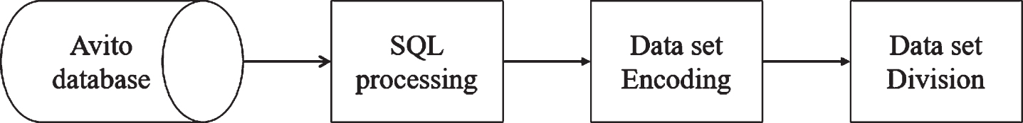
Data processing of DFIN.

(1) Build the Dataset

This paper uses the Avito dataset, and the original data is stored in the database. Because the data features are scattered in various data tables, it is necessary to connect related data tables when querying the database. The data tables mainly involved in this paper are SearchStream, SearchInfo, UserInfo, AdsInfo and Category.

Two points need to be paid attention to when querying the database: The first is the adjustment of the position of the feature in the dataset. The features in Avito are divided into single category, multi-category and continuous features. It is necessary to place single category and continuous features before multi-category features when querying, in order to make the data format more uniform and facilitate the realization of the embedding layer. The second is to sort the query results according to ViewDate to facilitate subsequent dataset division.

(2) Dataset Encoding

The initial dataset is obtained by processing the database data, and then the dataset needs to be encoded to obtain sparse data. The single category and multi-category data are respectively processed with one-hot [6] and multi-hot [20] encoding to obtain numerical data. The unified processing method for continuous data is to perform one-hot encoding after discretization, which is also to facilitate the realization of the embedding layer.

(3) Dataset Division

The common dataset division methods are cross-validation method and set-out method, the latter is used in this paper. The cross-validation method is to randomly divide the dataset into k mutually exclusive subsets and set aside one copy each time as the validation set.This method is usually used when the amount of data is small, so that the data in the dataset can be fully learned. The hold-out method is to divide the data according to a certain proportion. One of the reasons why this paper does not use cross-validation is that the amount of Avito data is large enough, and the other reason is to consider the time sequence of the data. Since the dataset has been sorted by time when constructing, the data after segmentation is also sequential. The reason for using the leave-out method is that the model needs to predict the click time that has not yet occurred when it is actually deployed, so it is hoped that the model can learn the prediction of future click events based on the previous data and improve the generalization ability of the model.

3.1.2 Network structure

The network structure of DFIN mainly includes input layer, embedding layer, cross layer and output layer, as shown in Fig. 2.

Fig. 2

Data processing of DFIN.

(1) Input Layer

The input data of DFIN is a high-dimensional sparse vector obtained through the data processing in Section 3.1, and no context is used, so the data is mainly related to the user and the current advertisement. The feature vector obtained after each original feature processing is regarded as a feature domain. Assuming that the original data has m features, after processing, the i-th feature will be converted into a sparse vector x_i, x_i represents the i-th feature domain, then The input data is shown in Eq. (1): $x = [x_{1}; x_{2}; . . .; x_{m}]$ (1)

Because the feature positions are adjusted during data processing, all one-hot encodings precede multi-hot encodings. Assuming that m′ features are one-hot encoded in the data, the first m′ feature domains have only one valid bit, and the following m – m′ feature domains have multiple valid bits.

(2) Embedding Layer

The embedding layer [19] maps the high-dimensional sparse vector of the input layer to a low-dimensional dense vector, and directly processes the data after the one-hot encoding. Assuming V_i is the embedding matrix of the i-th feature domain, and x_i represents the one-hot encoding of the i-th feature, the embedding vector can be expressed as Eq. (2): $e_{i} = V_{i} x_{i}$ (2)

Because x_i has only one valid bit, the embedding vector is actually the column vector corresponding to the valid bit in V_i, and its structure is shown in Fig. 3. Because x_i is a single category feature before one-hot encoding, it actually maps each value of the feature to a low-dimensional dense vector, and selects a specific low-dimensional dense vector as the embedding vector according to the feature value during embedding.

Fig. 3

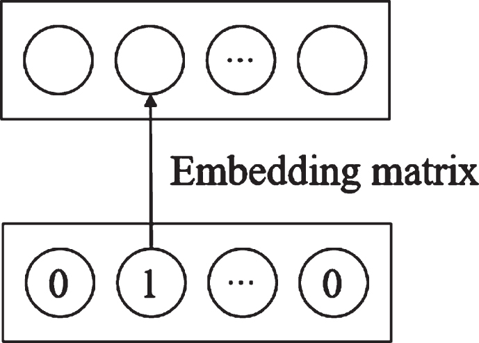
Single category feature embedding.

The embedding method of numerical data is the same as that of single category data, because the input of the cross layer requires the dimension of each feature domain to be the same.

Multi-category features are multi-hot encoded and have multiple valid bits. If the above embedding process is still performed, a low-dimensional dense vector of the same dimension can be obtained, which is essentially the result of adding column vectors corresponding to several valid bits. However, the number of valid bits is different for multi-hot encoding features, and there is only one bit in one-hot encoding. Therefore, when embedding multi-hot encoding features, multiple feature values need to be averaged for normalization. Assuming that V_i is the embedding matrix of the i-th feature domain, and x_i represents the multi-hot encoding of the i-th feature, the embedding vector can be expressed as shown in Eq. (3): $e_{i} = \frac{1}{q} V_{i} x_{i}$ (3)

Where q represents the number of valid bits in multi-hot encoding, and q=1 is the embedding method of one-hot encoding.

Finally, the output of the embedding layer can be expressed as the connection of a series of embedding vectors, as shown in Eq. (4): $e = [e_{1}; e_{2}; . . .; e_{m}]$ (4)

Where e_iεR^d, d represents the dimension of the embedding vector.

(3) Cross Layer

The cross layer is composed of an attention network and a residual network. The attention network is mainly used to solve the problem of high-order feature interactions, and the residual network is used to retain low-order feature interactions.

•Attention Network

The attention network in the deep feature crossover network uses a multi-headed self-attention network [2], which is to map features into different subspaces to obtain multiple interactions between features. The input of the multi-head self-attention network is a sequence, and the output is a sequence of equal length. But the output of the embedding layer is not a sequence and cannot be used as the input of the cross layer. Therefore, it is necessary to reshape the output of the embedding layer, as shown in Fig. 4. During embedding, each feature domain is mapped to an embedding vector with the same dimension, and each feature domain is regarded as an element in the sequence in the multi-head self-attention network.

Fig. 4

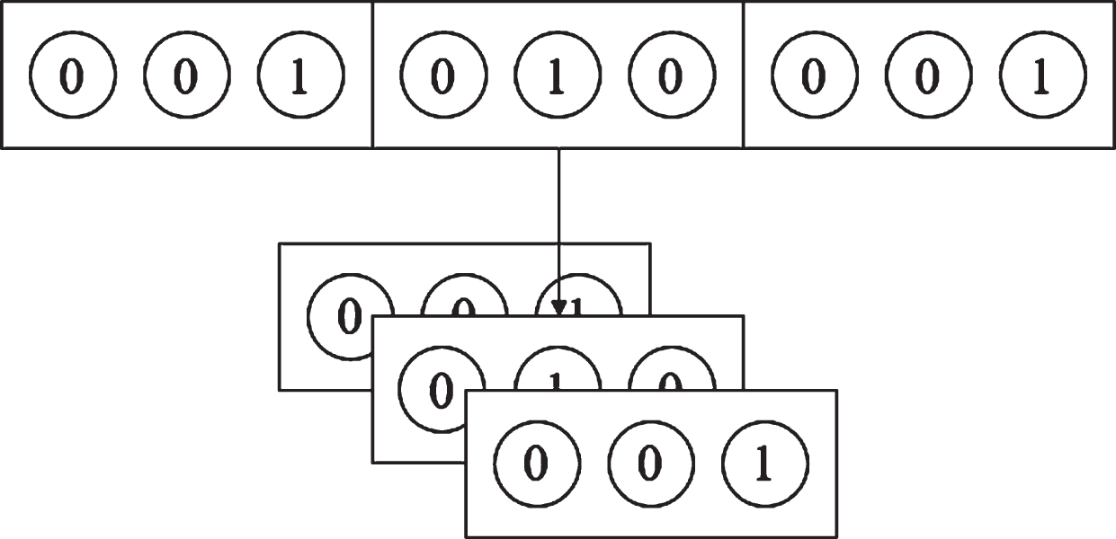
Reshape operation.

The output of the h-th header whose Key is e_i is shown in Eq. (7): $α_{ik}^{h} = \frac{\exp ({sim}^{h} (e_{i}, e_{k}))}{\sum_{l = 1}^{m} \exp ({sim}^{h} (e_{i}, e_{l}))}$ (5) ${sim}^{h} (e_{i}, e_{k}) = 〈 W_{Query}^{h} e_{i}, W_{Key}^{h} e_{k} 〉$ (6) ${\tilde{e}}_{i}^{h} = \sum_{k = 1}^{m} α_{ik}^{h} (W_{Value}^{h} e_{k})$ (7)

Where $W_{Query}^{h}, W_{Key}^{h}, W_{Value}^{h} ε R^{d^{'} \times d}$ , transform the original embedding space R^d to a new R^d′ space, then ${\tilde{e}}_{i}^{h} ε R^{d^{'}}$ . The above similarity function involves the interaction of the two embedding vectors e_i and e_k, the similarity function in the multi-head self-attention network introduces $W_{Query}^{h}$ and $W_{Key}^{h}$ , which are learned through the network and different in each head, So many kinds of interactions of e_i and e_k can be obtained.

Assuming that the multi-head self-attention network has a total of H heads, the output of e_i after being processed by the network is shown in Eq. (8): $\tilde{e_{i}} = [{\tilde{e}}_{i}^{1}; {\tilde{e}}_{i}^{2}; . . .; {\tilde{e}}_{i}^{H}]$ (8)

•Residual Network

As shown in Fig. 2, the residual network [31] adds the output of the embedding layer and the output of the multi-head self-attention network, thereby retaining the features that have not been feature-crossed. With the continuous addition of cross layers, the order of feature interaction will gradually increase. At this time, the residual network can continue to pass low-order feature interactions backward, thus ensuring that the network can capture both low-order and high-order feature crossovers at the same time.

There are two points to pay attention to in actual implementation: first, the output of the embedding layer is reshaped and used as the input of the residual network. Secondly, because the dimensions of e_m and ${\tilde{e}}_{m}$ are not necessarily the same, the addition operation cannot be directly performed. Introducing a W_res to change e_m, the output of the residual network is shown in Eq. (9): $e_{i}^{res} = ReLU (\tilde{e_{i}} + W_{res} e_{i})$ (9)

Where W_resεR^d′H×d, ReLU (x) = max (0, x) is a non-linear activation function.

(4) Output Layer

The final output of the ad CTR prediction model is an estimated value between 0-1, so the output layer uses a fully connected layer with only one output unit, and uses sigmoid as the activation function, which means that the output layer is essentially logistic regression. Therefore, the part before the output layer of DFIN can be regarded as automatic feature engineering, and finally logistic regression is used as the classifier of the model. The cross layer treats the entire feature as a sequence, each feature domain is an element in the sequence data, and the output of the cross layer is still sequence data. In the output layer, the sequence data is directly connected as a cross feature and input to the fully connected layer.

According to the cross layer, the i-th element in the output sequence is $e_{i}^{res}$ , and the input of the output layer is shown in Eq. (10): $e_{o} = [e_{1}^{res}; e_{2}^{res}; . . .; e_{m}^{res}]$ (10)

The expression of the output layer is shown in Eq. (11): $\hat{y} = σ (w^{T} e_{o} + b)$ (11)

Where wεR^d′Hm, b is the bias, and σ = 1/(1 + e^-x) represents the sigmoid function.

3.2 Deep context interaction network

This section first proposes the Deep Context Interaction Network based on pooling (DCIN-Pooling), which uses pooling to process context. Subsequently, the attention mechanism is used to improve the pooling, and the Deep Context Interaction Network based on attention mechanism(DCIN-Attention) is proposed, which is also the final model of this paper.

3.2.1 Data processing

The input data of DCIN is to add context on top of the input data of DFIN. In this paper, the input data in DFIN is called target advertisement data, because it is related to the current advertisement. The data processing flow of DCIN is basically the same as that of DFIN. The main difference is that in the step of constructing the dataset, because DCIN needs to query context.

The context used in this paper includes three types, namely, other ads in the current search page, ads clicked by users in the past, and ads not clicked by users in the past. The reason for using multiple contexts is to capture a variety of user preferences. Other ads on the search page can be found by SearchID, because each search will have a unique SearchID. The ads that users clicked and did not click in the past can be found by UserID, SearchDate, and IsClick. Because other ads on the current page are used as a separate type of context in this paper, the date here is SearchDate, which means to find the previous search Click or not click on the ad, if you use ViewDate, it may contain other ads on the current page.

Since the context is sequence data, in order to facilitate processing, the sequence length of various context is set to a fixed value, i.e., the too long sequence data is truncated, and the too short sequence data is filled. After aligning the context, the feature position needs to be adjusted, and single-category features and continuous features are placed in front of multi-column features. After that, the target advertisement feature is encoded in the same way as in Section 3.1, and then the sequence data is flattened and converted into a one-dimensional vector. Because the sequence data has a fixed length, the sequence can be identified by position in the network. The flow of the entire data processing is shown in the Fig. 5.

Fig. 5

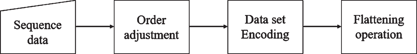
Data processing of DCIN.

3.2.2 Network structure

DCIN adds a processing module for each type of context, so the number of context types can be customized in actual implementation. The context processing is mainly divided into two methods: pooling and attention mechanism. Pooling is the basic processing method, and the attention mechanism is an improvement of pooling. Pooling directly averages the context to obtain the user interest vector, which reflects the user’s overall interest. But the user interest vector captured by pooling has nothing to do with the target advertisement data. The attention mechanism calculates the similarity between each context and the target advertisement data as the weight, and finally performs a weighted average to obtain the user interest vector. Compared with pooling, the attention mechanism can better reflect users’ current interests.

Deep Context Interaction Network Based on pooling

The biggest difference between the structure of DCIN-Pooling and DFIN is that context is added to the data of the input layer and a pooling layer is added after the embedding layer. The network structure is shown in Fig. 6. It can be seen from the structure diagram that the various context added in the input layer are processed by the embedding layer, then input to the pooling layer and converted into multiple user interest vectors. The network part after the pooling layer is the same as the network part after the embedding layer in DFIN, which mainly performs feature interaction and produces the final output, and the training method of DCIN-Pooling is also the same as DFIN. Therefore, only the structure before the cross layer in DCIN-Pooling is described.

Fig. 6

The network structure of DCIN-Pooling.

(1) Input Layer

The input layer of DCIN-Pooling mainly adds context. other ads on the current search page shows the user’s current interest, ads that the user has clicked in the past shows user’s historical interest and ads that the user did not click shows preferences that are not of interest to the user.

According to the data processing process in Section 4.1, the context and the current target advertisement data are processed into one record, and then uses location to identify context. However, in order to facilitate understanding, different context and target advertisement data are represented separately in the network diagram.

Assuming that the target advertisement feature is x_t, the features of other ads on the current search page, the user’s past clicks on the ads, and the user’s past non-clicked ads are respectively represented as x_pi, x_ci, and x_ui, and the input layer can be represented as shown in Eq. (12):

$\begin{matrix} x = [x_{t}; x_{p 1}; . . .; x_{{pn}_{p}}; x_{c 1}; \\ . . .; x_{{cn}_{c}}; x_{u 1}; . . .; x_{{un}_{u}}] \end{matrix}$ (12)

Where n_p, n_c, and n_u represent the sequence lengths of other ads on the current search page, the user’s past clicks on the ads, and the user’s past unclicked ads.

(2) Embedding Layer

The embedding layer of DCIN-Pooling is actually the same as the embedding layer of DFIN, except that the context is drawn as a sequence in the network structure. But in fact, the context has been expressed in the form of a record. So the embedding layer only needs to perform the same operations as the embedding layer of DFIN, but with more feature domains. Treat each feature in the context as a feature of the record, and then embed it one by one to get the final embedding vector, which can be expressed as shown in Eq. (13): $e = [e_{t}; e_{p 1}; . . .; e_{{pn}_{p}}; e_{c 1}; . . .; e_{{cn}_{c}}; e_{u 1}; . . .; e_{{un}_{u}}]$ (13)

Where e_t represents the embedding vector of the target advertisement, e_pi, e_ci, and e_ui represent the embedding vectors of other ads on the current search page, the user’s past clicks on the ads, and the user’s past non-clicking on the ads.

(3) Pooling layer

The context is a sequence, which cannot directly reflect the user’s interest, so the sequence data needs to be converted into an interest vector through the pooling layer. The pooling layer is most commonly used in CNN [17, 28] to retain important information in the process of dimensionality reduction of the data. In this section, it is used to reduce the dimensionality of two-dimensional sequence data into one-dimensional vector data.Common pooling methods include Max Pooling, Sum Pooling, and Average Pooling. In this paper, Average Pooling is used. Compared with Sum Pooling, there is an average operation, which can be regarded as normalizing the embedding vector. After the Average Pooling process, the three types of context are expressed as Eqs. (14), (15) and (16): $e_{p} = \frac{1}{n_{p}} \sum_{i = 1}^{n_{p}} e_{pi}$ (14) $e_{p} = \frac{1}{n_{p}} \sum_{i = 1}^{n_{p}} e_{pi}$ (15) $e_{p} = \frac{1}{n_{p}} \sum_{i = 1}^{n_{p}} e_{pi}$ (16)

e_p, e_c, and e_u are all vectors, and the composition of each vector is the same as d, which is composed of a series of feature domains and the embedding vector dimension of each feature domain is the same.Therefore, by connecting these vectors, a vector in the same form as the output of the embedding layer in DCIN can be obtained, as shown in Eq. (17). $e_{pooling} = [e_{t}; e_{p}; e_{c}; e_{u}]$ (17)

After reshaping e_pooling into a sequence, it can be input to the cross layer. Because this sequence contains the user interest vector, more feature interactions can be obtained, which makes the network perform better. However, when the context is pooled, the target advertisement data is not considered, so the attention mechanism can be used to improve the pooling.

Deep Context Interaction Network Based on Attention Mechanism

The attention mechanism [3, 13] can be regarded as a weighted pooling, so the use of the attention mechanism to improve the pooling can better capture the user’s interest related to the target advertisement. Compared with DCIN-Pooling, DCIN-Attention only changes the pooling layer, and the other parts are exactly the same. Its network structure diagram is shown in Fig. 7, so only how to use the attention mechanism to capture user interest is introduced.

Fig. 7

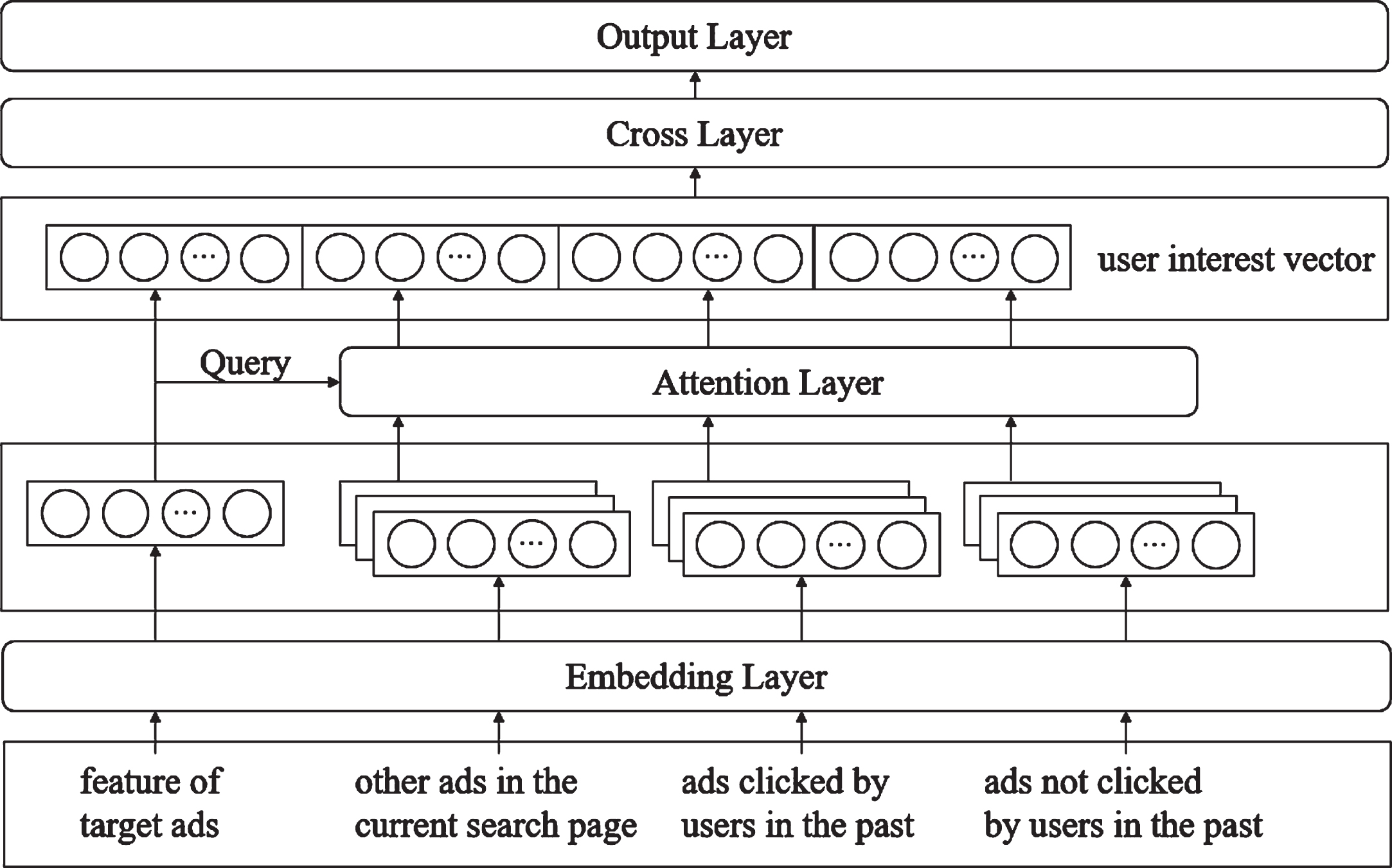
The network structure of DCIN-Pooling.

DCIN-Attention uses the attention mechanism to convert context into user interest vectors. When using the attention mechanism, the target advertisement data is used as Query to filter out user interests related to the target advertisement. Similar to the introduction of a pooling layer for each type of context in DCIN-Pooling, an attention layer is introduced for each type of context in DCIN-Pooling to capture various interest preferences of users. The output of the embedding layer is the same as DCIN-Pooling, i.e., the input of the attention layer is as shown in Eq. (13).

When using the attention mechanism to convert each context into a user interest vector, e_t is Query, the context formed respectively by e_pi, e_ci, and e_ui represent the Key and Value in the corresponding attention network. The results of processing each context are shown in Eqs. (18), (19) and (20): $e_{p} = \sum_{n_{p}}^{i = 1} sim (e_{t}, e_{pi}) e_{pi}$ (18) $e_{c} = \sum_{n_{c}}^{i = 1} sim (e_{t}, e_{ci}) e_{ci}$ (19) $e_{u} = \sum_{n_{u}}^{i = 1} sim (e_{t}, e_{ui}) e_{ui}$ (20)

The similarity function is realized by MLP. The main reason why inner product and cosine similarity are not used here is that the dimensions of e_t, e_pi, e_ci, and e_ui are not necessarily the same. These features are connected and processed as the input of the multilayer perceptron, and the forms are represented in Eqs. (21), (22) and (23):

$sim (e_{t}, e_{pi}) = \exp (h^{T} ReLU (W_{tp} + b_{tp 1}) + b_{tp 2})$ (21) $sim (e_{t}, e_{ci}) = \exp (h^{T} ReLU (W_{tc} [e_{t}; e_{ci}] + b_{tc 1}) + b_{tc 2})$ (22) $sim (e_{t}, e_{ui}) = \exp (h^{T} ReLU (W_{tu} [e_{t}; e_{ui}] + b_{tu 1}) + b_{tu 2})$ (23)

Where W_tp, W_tc, W_tuεR^k′×2mk and hεR^k′, and it is assumed here that each type of context has the same characteristics as the target advertisement. Finally, connect the output of the attention layer to get the same result as DCIN-Pooling, and then perform the same processing as DCIN-Pooling to get the output of DCIN-Attention. The loss function and training method are the same as DCIN-Pooling.

4 Experimental results and analysis

The Deep Context Interaction Network (DCIN) model proposed in this paper is mainly to improve the feature interaction and context processing problems in the advertising CTR prediction. In this chapter, a series of comparative experiments are designed to verify the effect of the model. Section 4.1 describes the experimental platform, Section 4.2 introduces the dataset used in the experiment, Sections 4.3 and 4.4 explain the training process and evaluation metrics of the model respectively, and finally analyze the results of the comparative experiment in Section 4.5.

4.1 Experimental setting

This paper uses a uniform environment configuration to ensure the effectiveness of the comparison experiment. In order to make model training faster and more efficient, the cloud server provided by MistGPU is used. The actual experimental environment is divided into two parts: hardware environment and software environment. A good hardware environment can ensure that the model is effectively trained, and its parameter configuration is shown in Table 2.

Table 2
Hardware environment configuration

Configuration Configuration Parameter

CPU Xeon Platinum 8160

RAM 24G

GPU RTX 2080Ti

Video memory 11G

Configuration	Configuration Parameter
CPU	Xeon Platinum 8160
RAM	24G
GPU	RTX 2080Ti
Video memory	11G

The software environment determines whether the code can run normally, and its specific parameters are shown in Table 3.

Table 3

Software environment configuration

Related configuration	Configuration Parameter
Operating System	Ubuntu16.04
Development Language	Python3.5
IDE	PyCharm2018.2
Algorithm Library	Tensorflow1.13 Scikit-learn0.22.2
Data Processing Library	Numpy1.19 Pandas1.0.3

4.2 Experimental dataset

This article uses the Avito Context Ad Clicks competition dataset in the Kaggle platform, which is a search advertising dataset. Compared with other classic advertising click-through rate datasets such as the Criteo dataset, the Avito dataset is more convenient for obtaining context. This is because the Criteo data set has processed the advertising data into a text file, and it is time-consuming to query the entire text file. However, the original form of the Avito dataset is a relational database, which can easily query context based on database statements. The database relationship diagram is shown in Fig. 8.

Fig. 8

Avito database diagram.

This paper uses 28 features in the Avito dataset. The features used include 1) ad features such as Ad ID, Ad Position, Ad Title, Ad Price, Ad Category, Ad Category Level, Ad Parent Category, Ad SubCategory Ad Params, 2) user features such as User ID, IP ID, IsUserLoggedOn, User Agent, User Agent OS, User Device, User Agent Family, 3)query features such as Search Query, Search Location, Search Location Level, Search Region, Search City, Search Category, Search Category Level,Search Parent Category, Search SubCategory and Serach Params. Among them, Price and HistCTR are continuous features, Serach Params and Ad Params are multi-category features, and the rest are single-category features.

Since the original dataset is large, there are hundreds of millions of actual production data, which cannot be fully utilized in the environment of this paper, so this paper directly samples the original dataset. Random sampling is not used in this paper, because the dataset contains ViewDate, a user browsing time field, and it predicts click events that did not occur, so the time sequence is maintained during sampling. In this paper, the first one million datasets are sampled, which is about one percent of the original data. The sampling form is shown in Fig. 9.

Fig. 9

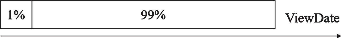
Dataset sampling.

In the model training process, in order to verify the effect of the model, the dataset needs to be divided into a training set, a validation set, and a test set. In this paper, time-based dataset partitioning is used instead of random data partitioning, in order to verify the effect of the model in predicting future click events. Divide 50% of the entire dataset into the training set and split the rest samples into validation and test sets of equal size. The result of the dataset division is shown in Fig. 10.

Fig. 10

Dataset division.

4.3 Model training

The loss functions used in this paper is logloss [25] function, the form of which is shown in Eq. (24):

$logloss = - \sum_{i = 1}^{n} [y_{i} \log \hat{y_{i}} + (1 - y_{i}) \log (1 - \hat{y_{i}})]$ (24)

Where y_i indicates that the i-th record is really a label, $\hat{y_{i}}$ means the estimated click-through rate is the output of the network.

The optimization algorithm used in this paper is the Adam algorithm [8, 23], which actually combines the momentum method [23] and RMSProp [23, 24]. There are two main reasons for choosing Adam in this paper: First, Adam is an adaptive algorithm that can escape the saddle point during the learning process, so that it is easier to find the minimum point of the loss function. Another reason is that momentum is added in the iterative update, which makes the learning of the network faster, thereby achieving faster and more stable finding of minimum points.

4.4 Evaluation metrics

Advertising CTR prediction is essentially a binary classification problem, so binary classification indicators can be used when evaluating the results. When estimating the CTR of an advertisement, the probability that a user clicks on it is more important, but does not necessarily need to predict whether to click or not. So the evaluation metrics does not use accuracy and F1. In this paper, Logloss and AUC are mainly selected as evaluation metrics, and the Logloss is also the loss function of the model.

Logloss: All models attempt to minimize the Logloss defined by Eq. (25), so it is used as a straightforward metric. The smaller the better.

AUC [4]: The Area Under the ROC Curve reflects the probability that a model ranks a randomly chosen positive instance higher than a randomly chosen negative instance. A higher AUC indicates a better performance. The calculation method of AUC is shown in Eq. (25): $AUC = \frac{\sum_{i ε positive} {rank}_{i} - \frac{M \times (M + 1)}{2}}{M \times N}$ (25)

Among them, rank represents the sequence number obtained by sorting the predicted probability from small to large, M represents the number of positive examples, N represents the number of negative examples, and i represents the i-th positive example.

4.5 Experimental results and analysis

All models for comparison experiments in this section are as follows:

FNN: FNN [26] is a FM-initialized feed-forward neural network and captures only high-order feature interactions.

Wide&Deep: Wide&Deep [16] combines LR (wide part) with DNN(deep part) to construct high-order feature interactions and low-order feature interactions.

DeepFM: DeepFM [11] combines FM (wide part) with DNN (deep part), and shares the same input and the embedding vector in its wide part and deep part. DeepFM can construct high-order feature interactions and low-order feature interactions, which is the benchmark model for feature interactions in this paper.

DFIN: DFIN uses the cross layer to improve DeepFM, and compares with DeepFM to show that it can better process feature interaction.

DCN-Pooling: Compared with the Deep Context Interaction Network(DCIN), the Deep Context Network(DCN) lacks the cross layer and uses the fully connected layer to process the context. The Deep Context Network based on pooling is the benchmark model of the context processing part in this paper.

DCN-Attention: DCN-Attention uses the attention mechanism to process the context. By comparing with the DCN-Pooling, it is verified that the attention mechanism can process the context more effectively.

DCIN-Pooling: DCIN-Pooling can handle feature interaction and context at the same time. A comparison with all the above networks can show that the DCIN-Pooling can effectively deal with these two problems.

DCIN-Attention: DCIN-Attention is the final model of this paper. By comparing with DCIN-Pooling, it shows that it is effective to use the attention mechanism to improve the pooling in the Deep Context Interaction Network.

4.5.1 Model hyperparameters

Hyperparameters refer to the parameters artificially set by the network before training, such as the number of layers of the network and the optimization algorithm. There are two main purposes for setting hyperparameters. The first is to determine the structure of the network; the second is to determine how the network is optimized. The hyperparameters related to the network structure are shown in Table 4.

Table 4
Model hyperparameters related to the network structure

FNN Wide&Deep DeepFM DFIN DCN DCIN

Pooling Attention Pooling Attention

Embedding Layer 20 20 20 20 20 20 20 20

Fully Connected Layer 3 3 3 N/A 3 3 N/A N/A

Cross layer N/A N/A N/A 3 N/A N/A 3 3

Context N/A N/A N/A N/A 3 3 3 3

	FNN	Wide&Deep	DeepFM	DFIN	DCN	DCIN
Embedding Layer	20	20	20	20	20	20	20	20
Fully Connected Layer	3	3	3	N/A	3	3	N/A	N/A
Cross layer	N/A	N/A	N/A	3	N/A	N/A	3	3
Context	N/A	N/A	N/A	N/A	3	3	3	3

In this paper, the features are embedded into 20-dimensional embedding vectors, and the number of feature unique value is 42301586, so the size of the embedding matrix is [42301586, 20]. The size of the embedding vector dimension mainly describes the complexity of the model. Setting it to 20 mainly considers the space complexity and overfitting. For larger data volume, it can be set to Bigger parameters.

FNN, Wide&Deep, DeepFM and DCN all use the fully connected layer to process feature interactions. In this paper, the number of fully connected layers is set as 3, each with dimensions 512, 256 and 1. Choosing three fully connected layers mainly considers the complexity of the network, and deeper networks are likely to cause over-fitting problems.

DFIN and DCIN replace the fully connected layer with the cross layer, so there are no parameters related to the fully connected layer. However, the cross layer parameters of these two types of networks are both set to three to keep the number of fully connected layers the same as above models, so that the comparison experiment results are more credible.

Because the actual structure of the Deep Context Network(DCN) and the Deep Context Interaction Network(DCIN) is related to the type of context, the information provided by the dataset needs to be considered in the specific implementation. The context of the dataset in this paper mainly contains three types, so the context hyperparameters of DCN and DCIN are both 3, and other models do not use context.

The hyper-parameters related to model training uses the same setting. The loss function and optimization algorithm in this paper use Logloss and Adam respectively, and the epochs and batch sizes are 10 and 128 respectively. The epochs is selected as 10 because the model will converge in about 10 rounds in the actual training process. Choosing a suitable batch is mainly for stable training and parallel computing with GPU. The actual selection will be limited by the size of GPU memory. In the experimental environment of this paper, setting it to 128 can achieve better results.

4.5.2 Model effect analysis

The results of the comparative experiment are mainly divided into three parts to explain. First, directly analyze the training results of different models to illustrate the effectiveness of the model proposed in this paper. After that, the loss function and AUC value changes of different models in the training process are analyzed to illustrate the learning ability of different networks. Finally, the network training time is compared and analyzed to directly quantify the complexity of the model.

The actual effects of different models on the dataset are shown in Table 5. In this paper, the comparative experiment is divided into three groups. The first group is to improve the feature interaction, the second group is to improve the context processing, and the third group is to merge the two parts. DCIN-Attention is the final model in this paper, and its AUC value is increased by 0.05 compared to DeepFM.

Table 5
Performance Comparison of Different Algorithms

Model Class Models AUC Logloss

Feature Interaction FNN 0.7395 0.5878

Wide&Deep 0.7416 0.5873

DeepFM 0.7432 0.5863

DFIN 0.7587 0.5746

Context DCN-Pooling 0.7333 0.5883

DCN-Attention 0.7442 0.5767

Feature Interaction +Context DCIN-Pooling 0.7734 0.5346

DCIN-Attention 0.7938 0.5261

Model Class	Models	AUC	Logloss
Feature Interaction	FNN	0.7395	0.5878
	Wide&Deep	0.7416	0.5873
	DeepFM	0.7432	0.5863
	DFIN	0.7587	0.5746
Context	DCN-Pooling	0.7333	0.5883
	DCN-Attention	0.7442	0.5767
Feature Interaction +Context	DCIN-Pooling	0.7734	0.5346
DCIN-Attention	0.7938	0.5261

First, make a histogram of the comparison experiment results of feature interactions as shown in Fig. 11. It is observed that Wide&Deep and DeepFM achieves higher AUC than FNN. And DeepFM achieves higher AUC than Wide&Deep. These results show that 1) combining a wide component and a deep component can improve the prediction performance, 2) FM in DeepFM can better capture low-order feature interactions than LR in Wide&Deep. DFIN outperforms DeepFM because it can construct arbitrary-order feature interactions through multi-head attention network and residual network. Through the similarity function in the multi-head attention network, high-order feature interactions can be constructed, and the order of features increases exponentially as the number of layers increases. The residual network is used to retain low-order feature interactions, so DFIN does not require the factorization machine part of DeepFM. To prove the contribution of the residual network, we removed it from the DFIN model and keep the other structures unchanged. As shown in Table 6, DFIN_w/ is the complete model while the DFIN_w/o is the model without residual network. It is observerd that the performance of models decrease if residual network are removed.

Fig. 11

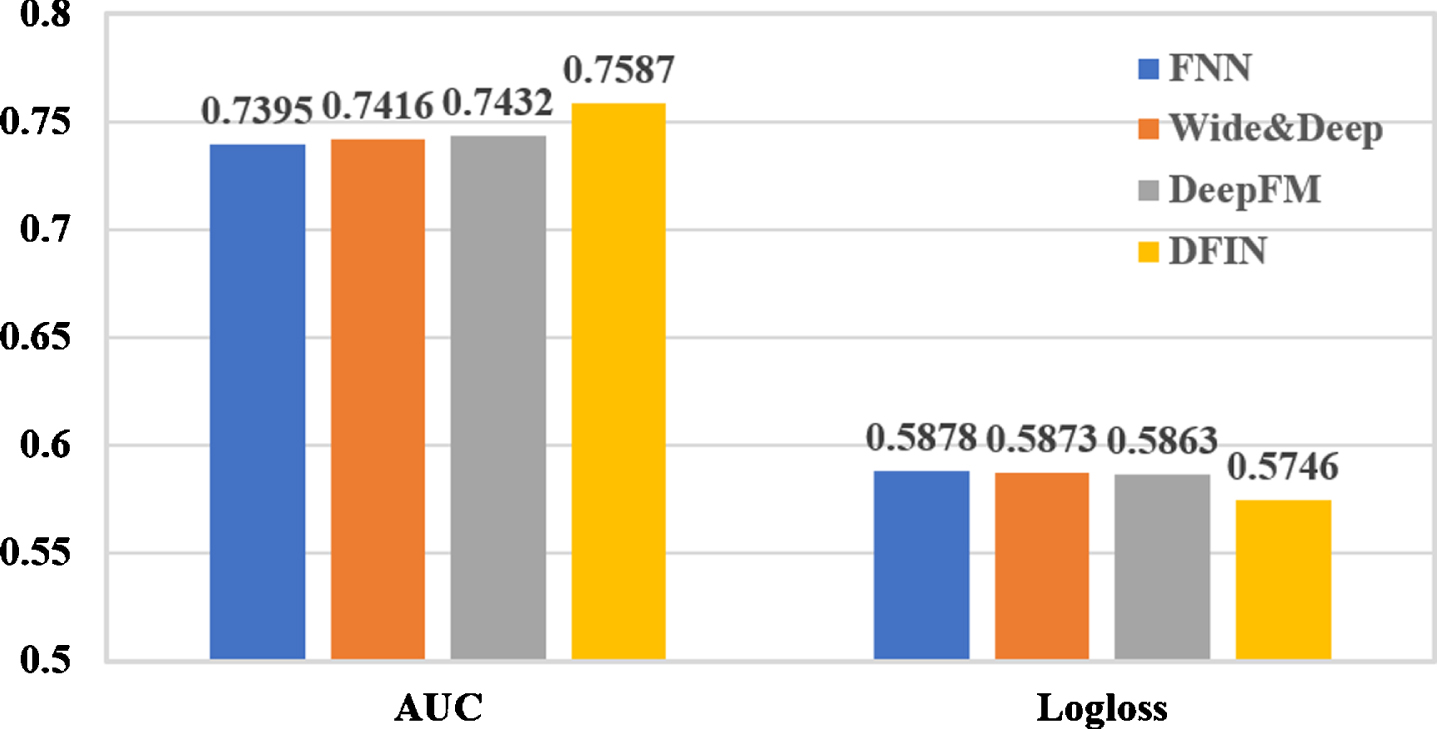
DeepFM and DFIN experiment results.

Table 6

Performance Comparison of DFIN_w/ and DFIN_w/o

Models	AUC	Logloss
DFIN_w/	0.7587	0.5746
DFIN_w/o	0.7551	0.5762

Second, analyze the two context-related models, and the histogram of the comparison experiment results can be represented as shown in Fig. 12. Compared with DCIN, DCN uses the fully connected layer instead of the cross layer when processing feature interaction. It is observed that DCN-Attention achieves higher AUC than DCN-Pooling. This result shows that the attention mechanism is more effective in capturing user interests than pooling, because the attention mechanism can capture user interests related to the target ad.

Fig. 12

DCN-Attention and DCN-Pooling experiment results.

The final third set of comparative experiments is to compare the model that only uses feature interaction or context with the model that uses feature interaction or context at the same time, i.e., to compare the effects of all models. AUC values of all models on the test set is shown in Fig. 13. The solid line in the figure represents the minimum value of a model that uses feature interaction and context at the same time, and the dotted line represents the maximum value of a model that only uses feature interaction or context. The solid line is higher than the dotted line, indicating that combining feature interaction and context can improve the performance of the model.

Fig. 13

AUC values of all models on the test set.

During the training process, the loss function values of different models on the training set and the AUC values on the validation set are recorded, which are respectively shown as shown in Fig. 14. When training the model, the validation set is mainly used to control early stopping. The data in the table is the result of using early stopping during model training. The Logloss and AUC values in the figure are the results of training without using the early stopping mechanism. The purpose is to be able to record the values of all rounds, and early stopping will stop training without getting better on the validation set.

Fig. 14

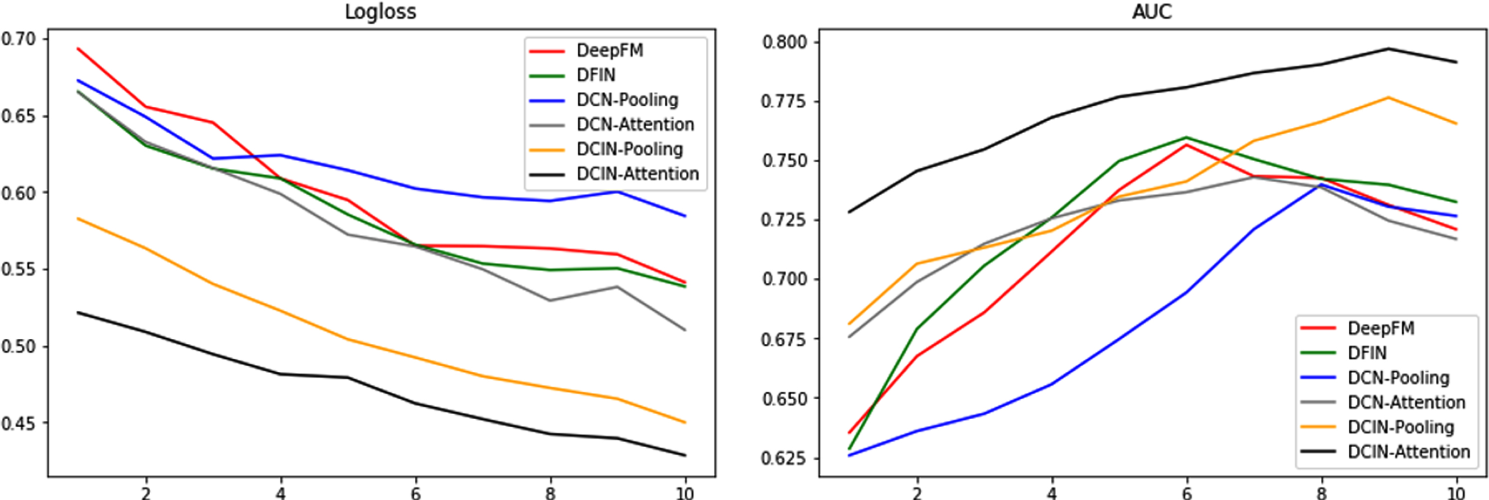
Training process.

The left image of Fig. 14 records the Logloss changes of the training set during the training process. It can be seen from the figure that the Logloss basically shows a downward trend during the training process, indicating that the model can effectively learn the training set. The right picture of Fig. 14 records the AUC change of the validation set during the training process, which reflects the generalization ability of the model. The figure basically shows a trend of rising first and then falling, indicating that the model is in the continuous learning process. Then it drops and the Logloss of the training set in the left figure also drops, indicating that the model has overfitting.

In order to solve the over-fitting problem in the model training process, a series of measures such as early stopping, regularization and discarding method are used in the actual training process of this paper. Among them, early stopping is used to control when the model stops training. In this paper, when the effect of several consecutive batches of the model is not improved, the training is stopped. It is essentially similar to selecting the model after the appropriate round through the training graph. Therefore, in this paper, the training graph has another function that can be used as a basis for the selection of epochs. According to the right graph of Fig. 14, the model basically has an inflection point around the 8th round, so the epochs in this paper is 10. So that the model can be fully trained.

Finally, the network training time is analyzed, and the histogram of the actual training time of different networks can be expressed as shown in Fig. 15. Since the model training time includes forward propagation and back propagation of the network, and back propagation can be regarded as the reverse process of forward propagation, its time complexity is roughly the same as that of forward propagation. Therefore, under the same hyperparameters, the model training time is directly proportional to the model complexity. The time complexity of DFIN is the same as DeepFM, while DCIN uses context, so its complexity is l+1 times, where l represents the number of contexts. Three types of context are used in this paper, so the training time of DCN and DCIN should be about 4 times that of DeepFM and DFIN. It can be seen from Fig. 15 that the training time of DeepFM and DFIN is about 15 minutes, while the training time of DCN and DCIN is about 60 minutes, which is similar to the analysis time complexity. Therefore, when the hidden layers of the network are roughly the same, the size of the context determines the network training time.

Fig. 15

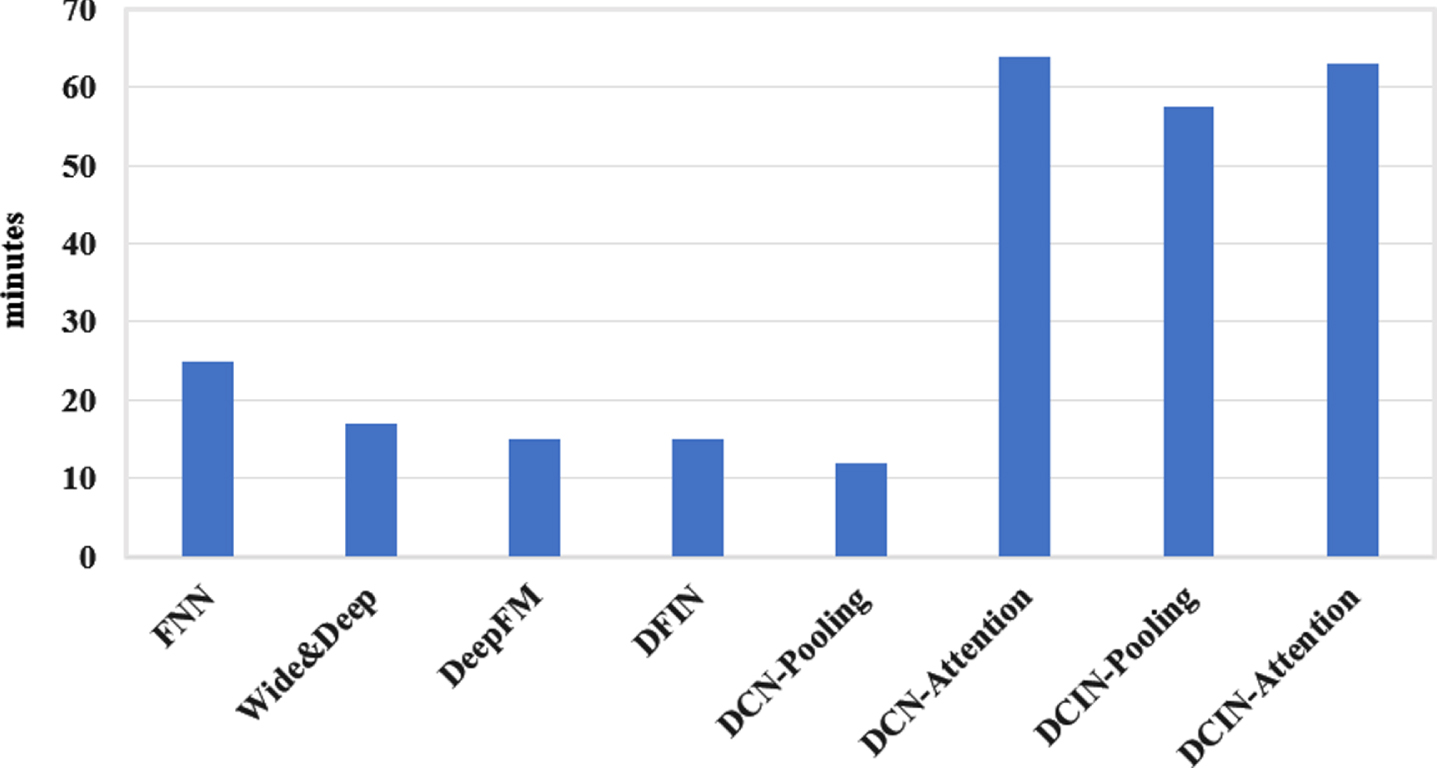
Training time comparison.

5 Conclusions and future works

In advertisements, feature interaction can often determine whether a user clicks, and context can reflect user interests, so these two issues are critical to the task of advertising CTR prediction. This paper mainly solves these two problems through the attention mechanism, and proposes two models, DFIN and DCIN. In order to verify the model, this paper conducted a series of comparative experiments on the Avito dataset. From the experimental results, it can be seen that DFIN can perform feature interaction better than DeepFM. Compared with DFIN, DCIN-Pooling and DCIN-Attention can effectively process context. At the same time, in DCIN, the attention mechanism is effective in improving pooling.

This paper mainly deals with two problems in ad click-through rate prediction, and finally proposes DFIN and DCIN. Although the two model in this paper is effective, there are still many aspects that can be improved. The possible improvements in the future can be listed as follows:

The embedding layer in this paper uses the original embedding layer. In the field of recommendation systems, user behavior data is abstracted into a graph data structure and difficult to directly use the embedding layer for processing, so graph embedding technology [1, 5] has gradually become popular. In computational advertising, the user’s past click data can be regarded as user behavior data to construct a graph data structure, and then graph embedding technology can be used to improve the embedding layer in this paper.

This paper uses pooling and attention mechanism to capture multiple user interests. Compared with YoutubeNet and DIN, this paper adds a variety of user interests, but does not distinguish between long-term and short-term user interests. The Sequential Deep Matching (SDM) [9] model proposed by Ali in 2019 captures long-term and short-term user interests [14] by constructing two sub-modules. This paper can also learn SDM and improve the context processing part of DCIN.

Footnotes

Acknowledgment

This work was supported by Guiding Project of Science and Technology Research Plan of Hubei Provincial Department of Education " Research on the Application of Intelligent Analysis of Surveillance Targets in Early Warning of College Students’ Abnormal Behaviors"(B2020163), and Social Science Fund Planning Project of Ministry of Education of People’s Republic of China "Research on Data Service and Guarantee for the Fourth Paradigm of Social Science"(20YJA870017)

This dataset was obtained from .

References

Grover

and Leskovec

, node2vec: Scalable Feature Learning for Networks, in: Knowledge Discovery and Data Mining (2016), 855–864.

Vaswani

, Shazeer

, Parmar

, et al., Attention is all you need, Advances in Neural Information Processing Systems (2017).

Zukovgregoric

, Bachrach

, Minkovsky

, et al., Neural Named Entity Recognition Using a Self-Attention Mechanism, in: International conference on tools with artificial intelligence (2017), 652–656.

Bradley

A.P.

, The use of the area under the ROC curve in the evaluation of machine learning algorithms, Pattern Recognition 1997, 1145–1159.

Perozzi

, Alrfou

, Skiena

, et al., DeepWalk: online learning of social representations, in: Knowledge discovery and data mining (2014), 701–710.

Seger

, An investigation of categorical variable encoding techniques in machine learning: binary versus one-hot and feature hashing (2018).

Zhou

, Xu

and Liu

, Incentive contract design for internet referral services: cost per click vs cost per sale, Kybernetes 49(02) (2019), 601–626.

Kingma

D.P.

and Ba

, Adam: A Method for Stochastic Optimization, in: International conference on learning representations (2015).

, Jin

, Yu

, et al., SDM: Sequential Deep Matching Model for Online Large-scale Recommender System, in: Conference on information and knowledge management (2019), 2635–2643.

10.

Zhou

, Zhu

, Song

, et al., Deep Interest Network for Click-Through Rate Prediction, in: Knowledge discovery and data mining (2018), 1059–1068.

11.

Guo

, Tang

, Ye

, et al., DeepFM: a factorization-machine based neural network for CTR prediction, Information Retrieval (2017).

12.

Liu

, Yun

, Lin

and Ding

, A survey on feature learning and technologies of online advertising click-through rate estimation, Journal of Zhejiang University(Science Edition) 46(05) (2019), 565–573.

13.

Mino

, Utiyama

, Sumita

, et al., Key-value Attention Mechanism for Neural Machine Translation, in: International joint conference on natural language processing (2017), 290–295.

14.

Ying

, Zhuang

, Zhang

, et al., Sequential Recommender System based on Hierarchical Attention Networks, in: International joint conference on artificial intelligence (2018), 3926–3932.

15.

Zhu

, Jin

, Tan

, et al., Optimized Cost per Click in Taobao Display Advertising, in: Knowledge discovery and data mining (2017), 2191–2200.

16.

Cheng

H.T.

, Koc

, Harmsen

, et al., Wide&deep learning for recommender systems., in: Proceedings of the 1st workshop on deep learning for recommender systems, (2016), 7–10.

17.

Goodfellow

, Bengio

and Courville

, Deep learning, MIT Press (2016), 321–362.

18.

iResearch, Annual Monitoring Report of China’s Online Advertising Market, iResearch Consulting Series Research Report 2019(06) (2019), 456–537.

19.

Wang

, Huang

, Zhao

, et al., Billion-scale Commodity Embedding for E-commerce Recommendation in Alibaba, in: Knowledge discovery and data mining (2018), 839–848.

20.

Feng

, Wei

, Guo

, et al., Rethinking Generalized Matrix Factorization for Recommendation: The Importance of Multihot Encoding (2019).

21.

Covington

, Adams

, Sargin

, et al., Deep Neural Networks for YouTube Recommendations, in: Conference on recommender systems (2016), 191–198.

22.

and Zheng

, The Original Climate, Operating Mechanism, and Evolution of Computational Advertising, Shandong Social Sciences 2019(11), 164–169.

23.

Dozat

, Incorporating nesterov momentum into adam, (2016).

24.

Tijmen

and Hinton

, RMSprop gradient optimization, (2014).

25.

Vovk

, The fundamental nature of the log loss function, Fields of Logic and Computation II (2015), 307–318.

26.

Zhang

, Du

, Wang

, et al., Deep Learning over Multi-field Categorical Data, in: European conference on information retrieval (2016), 45–57.

27.

and Chua

T.-S.

, Neural Factorization Machines for Sparse Predictive Analytics, Research and Development in Information Retrieval (2017).

28.

Le Cun

, Le Net-5, Convolutional Neural Networks (2015).

29.

, Cai

, Ren

, et al., Product-Based Neural Networks for User Response Prediction, in: International conference on data mining (2016), 1149–1154.

30.

Shan

, Hoens

T.R.

, Jiao

, et al., Deep Crossing: Web-Scale Modeling without Manually Crafted Combinatorial Features, in: Knowledge discovery and data mining, (2016), 255–262.

31.

Tai

, Yang

, Liu

, et al., Image Super-Resolution via Deep Recursive Residual Network, in: Computer vision and pattern recognition (2017), 2790–2798.