Imbalanced data enhancement method based on improved DCGAN and its application

Abstract

Machinery operates well under normal conditions in most cases; far fewer samples are collected in a fault state (minority samples) than in a normal state, resulting in an imbalance of samples. Common machine learning algorithms such as deep neural networks require a significant amount of data during training to avoid overfitting. These models often fail to detect minority samples when the input samples are imbalanced, which results in missed diagnoses of equipment faults. As an effective method to enhance minority samples, Deep Convolution Generative Adversarial Network (DCGAN) does not fundamentally address the problem of unstable Generative Adversarial Network (GAN) training. This study proposes an improved DCGAN model with improved stability and sample balance for achieving greater classification accuracy over minority samples. First, spectral normalization is performed on each convolutional layer, improving stability in the DCGAN discriminator. Then, the improved DCGAN model is trained to generate new samples that are different from the original samples but with a similar distribution when the Nash equilibrium is reached. Four indices—Inception Score (IS), Fréchet Inception Distance Score (FID), Peak Signal to Noise Ratio (PSNR), and Structural Similarity (SSIM)—were used to quantitatively evaluate of the generated images. Finally, the Balance Degree of Samples (BDS) index was proposed, and the new samples are proportionally added to the original samples to improve sample balance, resulting in the formation of several groups of datasets with different balance degrees, and Convolutional Neural Network (CNN) models are used to classify these samples. With experimental analysis on the reciprocating compressor, the variance of lost data is found to be less than 1% of the original value, representing an increase in stabilityof the model to generate diverse and high-quality sample images, as compared with that of the unmodified model. The classification accuracy exceeds 95% and tends to remain stable when the balance degree of samples is greater than 80%.

Keywords

Imbalanced data enhancement fault diagnosis DCGAN CNN

1 Introduction

In modern technology and industry, equipment has become increasingly large-scale, complicated, high-speed, automatic, and intelligent. A consequence of appropriate functioning is a decreased number of fault samples, resulting in a sample imbalance. Common machine learning algorithms such as deep neural networks require a large amount of data to train models in order to avoid overfitting. These models often fail to detect minority samples, thereby increasing the probability of missed diagnoses when the input samples are imbalanced. Once a missed fault develops to a significant degree, unplanned outages or production interruptions can occur, resulting in significant economic losses. This issue of class imbalance can be resolved by expanding the minority dataset. Sampling methods, including oversampling and undersampling, help reduce the shortage caused by imbalanced data. Oversampling results in data duplication, leading to overfitting of the model; by contrast, undersampling results in a loss of training data, affecting the global representation of the model [1]. Although the synthesis method based on SMOTE [2, 3] solves these problems to a certain extent, the distribution characteristics of neighboring samples are not addressed, which increases the probability of sample overlap, contributing to the poor availability of new training samples [4].

In the field of computational vision, data augmentation is used to manually expand datasets by generating equivalent data from limited data. This technique can be roughly divided into two categories: the first category is data augmentation based on basic image processing techniques, such as random clipping, scaling, rotation, contrast transformation, illumination color transformation, and noise addition operations [5]. Despite the desirable data enhancement results of this approach, limitations still exist. For example, data augmentation using image processing only performs transformation on the basis of the original image with repeatability and single data distribution [6]. The second category is data augmentation algorithms based on deep learning, such as generative adversarial network (GAN). In recent years, the GAN has led to significant advances in many fields, including image generation [7], video synthesis [8], and speech processing [9]. Unlike other methods, the GAN can learn the distribution of actual samples and generate near-actual samples. Nevertheless, the GAN is less reliable in practical applications due to unstable training, slow convergence, and limited quantitative evaluation criteria [10].

GAN currently comprises numerous variations that consist of Deep Convolution GAN (DCGAN), Wasserstein GAN (WGAN), Wasserstein GAN-Gradient Penalty (WGAN-GP), as well as BigGAN. DCGAN initially introduced a deep convolutional network into GAN, which ensured the quality and diversity of generated images, nevertheless the defect was that the model training was unstable [11]. WGAN primarily improved GAN in terms of the loss function, and Wasserstein distance was adopted to replace JS divergence in conventional GAN. On that basis, several problems were theoretically solved, which include mode collapse, gradient disappearance, as well as gradient explosion, whereas the improper pruning of the weight will result in gradient dispersion [12]. WGAN-GP was added with gradient penalty term based on WGAN network, thereby meeting the Lipschitz continuity condition and solving the unbalanced WGAN training, but the convergence speed was slow, and the samples generated exhibited the insufficient diversity [13]. BigGAN refers to a GAN with a significant large scale, which exploits skill training, including truncation and orthogonal regularization, to train and generate high-definition images. However, its defects consist of the large number of parameters, the difficulty in training, the need to use multiple Graphics Processing units (GPUs) for training, as well as the high implementation cost [14].

Compared with the general GAN network, the improved model has stronger generation capability. However, a range of problems remain, which comprise the unstable training, the mode collapse, the poor quality of generated images, as well as training difficulties. Accordingly, to achieve a low-cost training model realization and the diversity and high quality of generated images, the DCGAN model was selected here for research. However, only the network structure and training skills are improved in DCGAN; the stability of the training process is not improved. It is necessary to focus on balancing the training process of the generator and discriminator. The main reason for the instability of the GAN is that the discriminator cannot satisfy the Lipschitz constraints [15, 16]. Spectral normalization, as proposed by Miyato et al. [17], normalizes the parameters in the discriminator such that the gradient of the mapping function satisfies the Lipschitz constraints, further stabilizing the training process of the discriminator. Studies have indicated that spectral normalization can help maintain the stability of the parameter matrix while satisfying the Lipschitz continuity [6 , 18]. Thus, the DCGAN model is improved in this study by performing spectral normalization on each convolution layer in the discriminator for model stabilization. Samples different from the original ones but with a similar distribution are generated for data enhancement, eventually affording greater stability and diagnostic accuracy.

Convolutional neural network (CNN) is one of the most effective deep learning methods, which directly processes the original monitoring signals without pre-processing and feature extraction and automatically mines the fault rules hidden behind the data. It integrates signal processing, feature extraction, and pattern recognition to achieve end-to-end fault diagnosis. In many application areas of machine learning, particularly in machine vision feild, CNN has become a focus of research. The remainder of this paper is structured as follows. Section 2 briefly explains the theoretical background of the methods used in this study. Section 3 details the proposed method. Section 4 describes the experiment design, data augmentation, and fault classification and analysis. Lastly, Section 5 presents the conclusions.

2 Theoretical background

2.1 Wavelet transform (WT)

In Due to limited sources and information, one–dimensional vibration signals collected from the equipment are transformed into two–dimensional time–frequency images via wavelet transform (WT). The new images contain both time and frequency domain information with rich features for use as the input of DCGAN. WT is a process wherein a translation b and a scale change α are achieved on a basic wavelet function, and the inner product of a signal x(t) is analyzed. $X (α, b) = \frac{1}{\sqrt{α}} \int_{- \infty}^{+ \infty} x (t) ψ (\frac{t - b}{α}) dt, α > 0$ (1) where α is the scale factor, with the function of stretching the basic wavelet function ψ(t). b reflects the translation; its value can be positive or negative. When α and b are continuous variables, the WT is continuous. In this study, information entropy is used as the evaluation criterion for selecting the optimal wavelet basis function. A larger information entropy produces more information in the image [19].

Let f(x, y) be an image with k gray levels, where the probability of gray level i (i = 1–k) is p_i. According to the principle of information theory, the information content of gray level i is expressed as $I (i) = \log (1 / p_{i}) = - \log (p_{i})$ (2)

The information entropy of this image is $H = \sum_{i = 0}^{k - 1} p_{i} \cdot \log (\frac{1}{p_{i}}) = - \sum_{i = 0}^{k - 1} p_{i} \cdot \log (p_{i})$ (3)

Four wavelet basis functions (cmor3-3, db10, sym8, and meyr) are used to perform wavelet transformation on the vibration signals of a reciprocating compressor testbed with a bolt looseness. Furthermore, the four types of information entropy of time–frequency images obtained by wavelet transformation are calculated, as shown in Table 1.

Table 1

Information entropy of four time–frequency images

Wavelet basis function	cmor3-3	db10	sym8	meyr
Information entropy	4.8877	4.2788	4.4028	4.2726

As shown in Table 1, the information entropy of the time–frequency image transformed by cmor3-3 is the greatest, indicating that this image contains the most information. Thus, this study uses cmor3-3 for wavelet transform.

2.2 Deep convolution generative adversarial network (DCGAN)

The DCGAN is an improved GAN model. The primary advantage of DCGAN is that the convolutional layer can extract features and generate near-actual images. The DCGAN model includes a discriminator (D) and a generator (G). D is composed of Conv2d layers, BN layers, LeakyReLU activation layers, and Sigmoid layer. G is composed of ConvTranspose2d layers, BN layers, ReLU activation layers, and Tanh layer. The principle underlying the DCGAN is described as follows: G receives a random noise z and generates an image G(z); D receives an image x and outputs D(x), indicating the probability that the image x is an actual image. 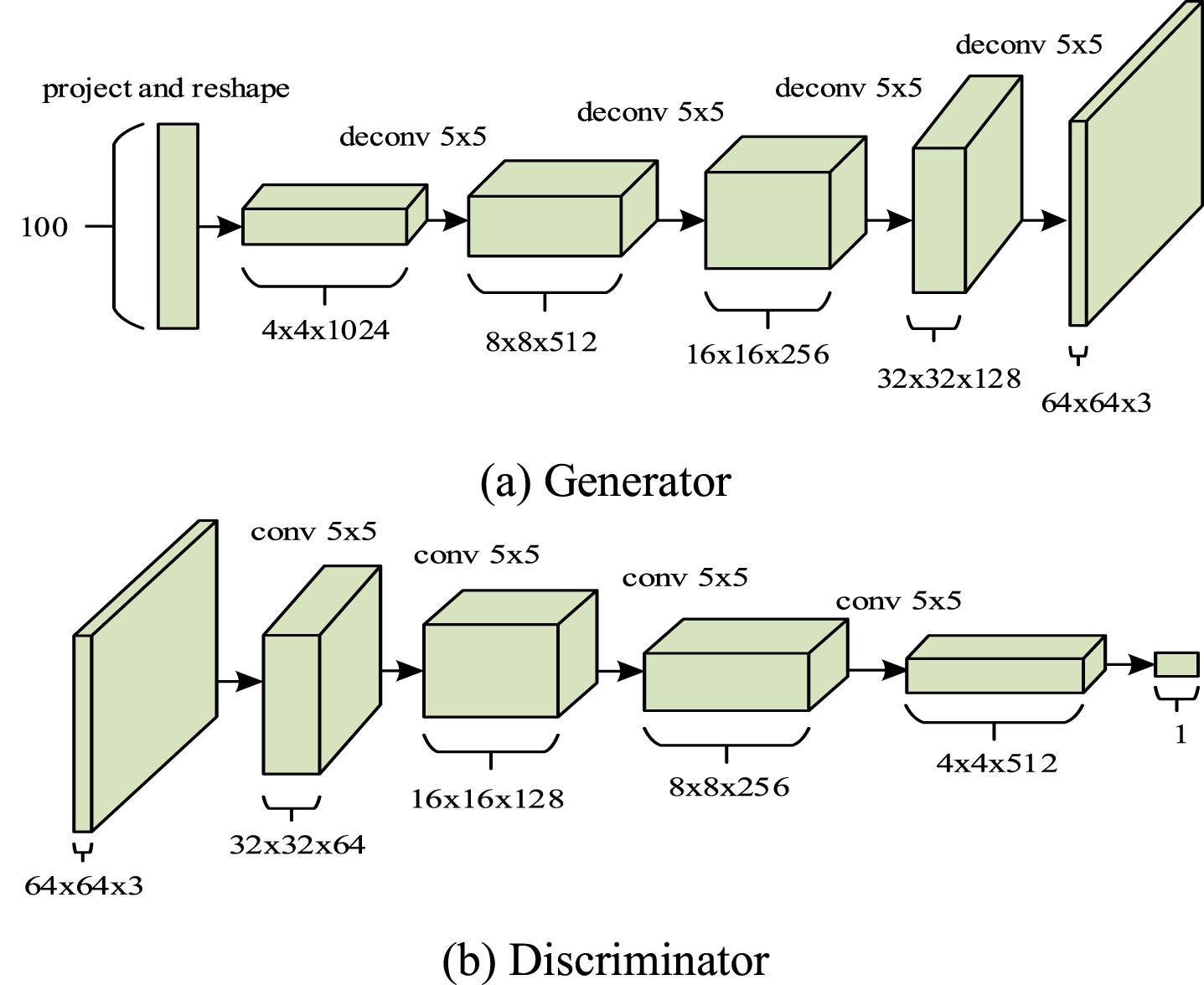The objective function is expressed as $\begin{matrix} min_{G} max_{D} V (D, G) = E_{x \sim p_{data (x)}} [log D (x)] + \\ E_{z \sim p_{z} (z)} [log (1 - D (G (z)))] \end{matrix}$ (4) where E (*) represents the expected value of the distribution function, P_data (x) represents the distribution of original images, and P_z(z) is the distribution of the generated images. The process of generating images using G and assessing images using D is illustrated in Fig. 1.

Fig. 1

Structure of the DCGAN.

As shown in Fig. 1, the input of the generator is a 100–dimensional random noise vector z with uniform distribution and an interval of [–1, 1]. The generator reshapes the vector z as the input, continuously performs deconvolution operations, and outputs data with a size of 64×64×3. The input dimension of the discriminator is consistent with the output of the generator. The output of the original samples is a vector with a length of 1 and a range of 0–1, indicating the probability that the input data is an original sample rather than a generated sample.

2.3 Convolutional neural network (CNN)

A basic CNN model consists of an input layer, a convolution layer, an activation layer, a pooling layer, a fully connected layer, and an output layer. Two–dimensional time–frequency images are used as the input. The convolution calculation is conducted through the convolution kernel, and the feature map is obtained by activating the function in the convolution layer. The convolution layer is expressed as $a_{j}^{l} = f (\sum_{i \in M_{j}} a_{i}^{l - 1} \times ω_{ij}^{l} + b_{j}^{l})$ (5) where $a_{j}^{l}$ is the output of the j neuron in the l layer, and $a_{i}^{l - 1}$ is the input of the i neuron in the l - 1 layer; M_j is the input feature map, l indicates the layer l, and ω indicates the weight matrix (the filter). $b_{j}^{l}$ is the network bias of the j neuron in the l layer, and f represents the activation function.

The pooling layer, also known as the downsampling layer, is used to extract local features, accelerate convergence, and establish spatial and structural invariance. The pooling layer is described as $a_{j}^{l} = f (β_{j}^{l} down (a_{j}^{l - 1}) + b_{j}^{l})$ (6) where down () represents the downsampling function, and β is the multiplicative bias of the network.

Located at the end of the network, the fully connected layer is generally used as the output for conducting regression and classification on the extracted features through layer-by-layer transformation and mapping.

3 Proposed method

3.1 Theoretical analysis of improved DCGAN model

In accordance with the stability theorem of the GAN, when the input and output satisfy the Lipschitz continuity, the control performance of the discriminator network is enhanced, and the training stability of the GAN increases accordingly. Because the LeakyReLU and Sigmoid activation functions have already met the Lipschitz constraints [20], the entire discriminator can be continuous on the condition that Lipschitz continuity is achieved for each convolutional layer. Thus, spectral normalization (SN) is performed for each convolution layer in the discriminator by replacing the BN Layer and normalizing the spectrum of the matrix with back propagation to fulfill the Lipschitz continuity requirement during the interlayer gradient transfer [21]; this is to prevent drastic changes in the discriminator’s parameters, which improves the stability of the GAN network. In this process, the structure of the convolution kernel is not destroyed [22]. The analysis is described as follows.

The improvement of the discriminator includes: the parameter θ is restricted to meet the Lipschitz restraints of function f, and a global regularity is imposed on the discriminator network, preventing the network parameters from strengthening along a certain direction. The Lipschitz constraint is expressed as $\frac{∥ f (x_{1}, θ) - f (x_{2}, θ) ∥}{∥ x_{1} - x_{2} ∥} ⩽ M$ (7) where x₁ and x₂ represent the model input, f(x₁, θ) and f(x₂, θ) represent the model output, and M is a constant.

Spectrum normalization normalizes the weight matrix of each convolution layer. The parameter matrix of convolution layer is A; the spectral norm σ (A) of matrix A is calculated as $σ (A) = \sup_{x \neq 0} \frac{{∥ A x ∥}_{2}}{{∥ x ∥}_{2}} = \sup_{{∥ x ∥}_{2} ⩽ 1} {∥ A x ∥}_{2}$ (8) where the matrix σ (A) is equal to the maximum singular value of the matrix A, and the Lipschitz continuity constant of the convolution layer is equivalent to the spectral norm of the convolution layer parameter matrix. The maximum singular value of the normalized convolution layer parameter matrix W_SN is 1, which is determined by solving the spectral norm σ (W) of the convolution layer parameter matrix W. W_SN is calculated as $W_{SN} = W / σ (A)$ (9)

The maximum singular value of the convolution layer is 1; the input and output of the convolution layer satisfy the Lipschitz continuity after spectral normalization. Thus, it can be inferred that the input and output of the discriminator network meet the Lipschitz continuity requirement.

3.2 Network structure of IM_DCGAN model

The spectrum of each convolution layer in the discriminator is normalized, the SN layer is added, and the BN layer is removed. The network structure is shown in Table 2. The improved DCGAN model is denoted as IM_DCGAN, and the parameters are set as follows: Adam is set to (0.5, 0.99), the convolution kernel is 4×4, the learning rate is 0.001, the batch size is 32, the decay round is 5, nz is 1024, and the size of the output image is (64, 64, 3).

Table 2
IM_DCGAN network structure

Generator Discriminator

ConvTranspose 2d 4×4, stride 1, pad 0, no bias. 1024->512 SN (Conv2d 4×4, stride 2, pad 1, no bias), 3->64

BN and ReLU LeakyReLU 0.2

ConvTranspose 2 d 4×4, stride 2, pad 1, no bias. 512->256 SN (Conv2d 4×4, stride 2, pad 1, no bias), 64->128

BN and ReLU LeakyReLU 0.2

ConvTranspose 2 d 4×4, stride 2, pad 1, no bias. 256->128 SN (Conv2d 4×4, stride 2, pad 1, no bias), 128->256

BN and ReLU LeakyReLU 0.2

ConvTranspose 2 d 4×4, stride 2, pad 1, no bias. 128->64 SN (Conv2d 4×4, stride 2, pad 1, no bias), 256->512

BN and ReLU LeakyReLU 0.2

ConvTranspose 2 d 4×4, stride 2, pad 1, no bias. 64->3 SN (Conv2d 4×4, stride 1, pad 0, bias), 512->1

Tanh Sigmoid

Generator	Discriminator
ConvTranspose 2d 4×4, stride 1, pad 0, no bias. 1024->512	SN (Conv2d 4×4, stride 2, pad 1, no bias), 3->64
BN and ReLU	LeakyReLU 0.2
ConvTranspose 2 d 4×4, stride 2, pad 1, no bias. 512->256	SN (Conv2d 4×4, stride 2, pad 1, no bias), 64->128
BN and ReLU	LeakyReLU 0.2
ConvTranspose 2 d 4×4, stride 2, pad 1, no bias. 256->128	SN (Conv2d 4×4, stride 2, pad 1, no bias), 128->256
BN and ReLU	LeakyReLU 0.2
ConvTranspose 2 d 4×4, stride 2, pad 1, no bias. 128->64	SN (Conv2d 4×4, stride 2, pad 1, no bias), 256->512
BN and ReLU	LeakyReLU 0.2
ConvTranspose 2 d 4×4, stride 2, pad 1, no bias. 64->3	SN (Conv2d 4×4, stride 1, pad 0, bias), 512->1
Tanh	Sigmoid

3.3 Procedure of the proposed method

The proposed method includes five main parts: data acquisition, wavelet transform, image generation, dataset constitution with multiple balance degrees, and fault classification, as shown in Fig. 2.

Fig. 2

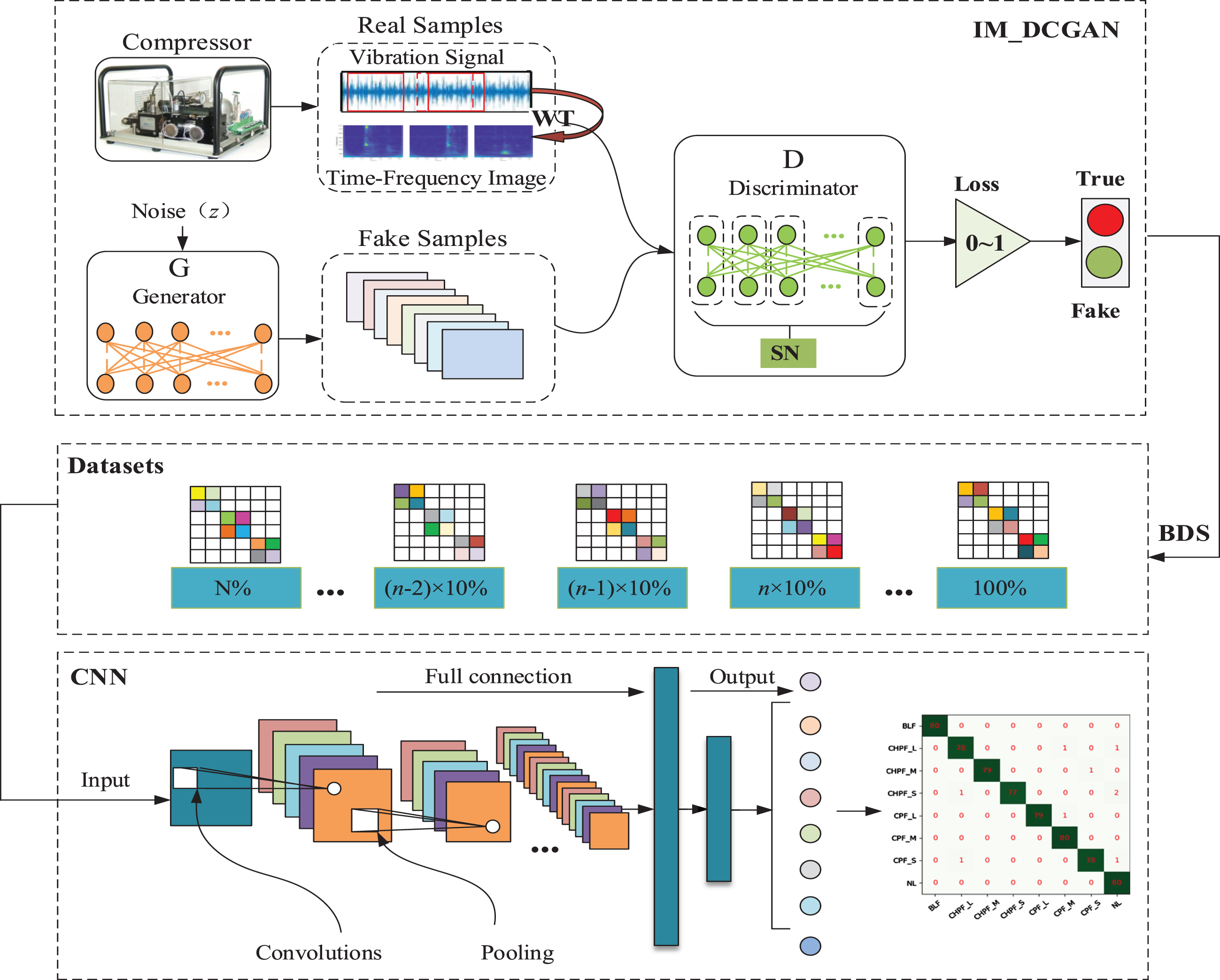
Flowchart of proposed method. Note: N% represents the percentage of original imbalanced samples, and n represents the number of intervals.

The process can be detailed as follows:

Step 1: Collecting the vibration signals of a reciprocating compressor using a vibration accelerometer sensor.

Step 2: Extracting fixed–length vibration signal samples using window sliding, and employing wavelet transform to convert one–dimensional signals into two–dimensional time–frequency images.

Step 3: Conducting spectral normalization for each convolutional layer in the discriminator of the DCGAN. When D(x) ≈ 0.5, the Nash equilibrium is reached, and new time–frequency images are generated, different from the original samples but with similar distribution.

Step 4: The new samples are proportionally added to the original datasets to improve the balance of the samples, forming several groups of datasets with different balance degrees.

Step 5: Inputting these datasets with different balance degrees into the CNN models for fault classification.

4 Experimental study

As shown in Fig. 3, the experimental system of the reciprocating compressor consists of a reciprocating compressor, signal monitor, data acquisition unit, and laptop. A single-cylinder, double-acting reciprocating compressor comprising a motor, crankshaft, crankshaft pin, connecting rod, crosshead, cylinder, piston assembly, buffer tank, pressure gauge, and flow regulating valve is used. It can simulate events such as abnormal crosshead clearances, abnormal crankshaft clearances, and bolt looseness on a chassis base. The top view of the reciprocating compressor is presented in Fig. 4.

Fig. 3

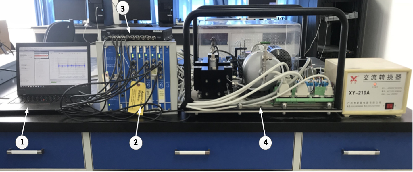
Experimental system: ➀ Laptop; ➁ Signal monitor; ➂ Data acquisition unit; ➃ Reciprocating compressor.

Fig. 4

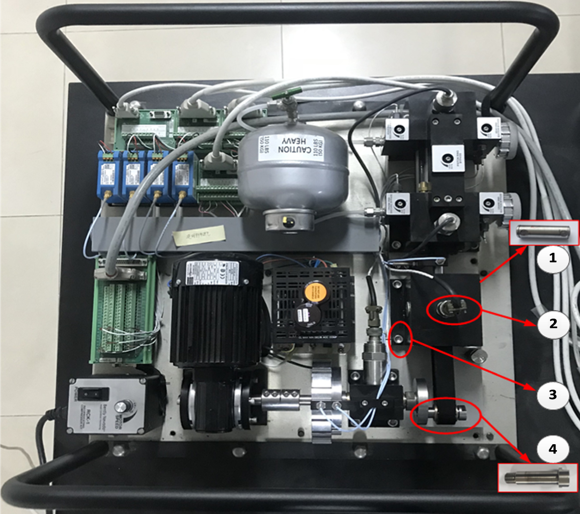
Top view of reciprocating compressor: ➀ Crosshead pin; ➁ Vibration acceleration sensor; ➂ Bolt; ➃ Crankshaft pin.

During the experiment, the vibration acceleration sensor (Fig. 4 ➁) installed on the reciprocating compressor (Fig. 3 ➃) collects and transmits the vibration signals to the signal monitor (Fig. 3 ➁) through the signal line and to the data acquisition unit (Fig. 3 ➂). The data acquisition unit transmits the vibration acceleration signals to the laptop (Fig. 3 ➀) for data analyses.

4.1 Experimental design

The parameters of the reciprocating compressor test bench are as follows: motor speed = 100 r/min and compressor discharge pressure = 20 psi. The vibration acceleration sensor is installed in the radial direction of the crosshead, as shown in Fig. 4 ➁. The sampling frequency is 20 kHz, and the sampling time is 10 s. The experiments are described as follows:

Normal operation: The vibration signals under normal equipment operation are collected.

Abnormal crosshead clearance: Different degrees of wear between the crosshead pin and the small head bush of the connecting rod are simulated using a crosshead pin with different diameters. The experimental position is shown in Fig. 4 ➀, and the parameters are presented in Table 3.

Abnormal crankshaft clearance: Crankshaft pins with different diameters are used to simulate different degrees of wear between the crankshaft pin and the big head bush of the connecting rod. The experimental position is shown in Fig. 4 ➃, and the parameters are presented in Table 4.

Bolt looseness on chassis base: Four bolts are fixed on the base of the crosshead chassis, and one of the bolts is loosened. The experimental position is shown in Fig. 4 ➂.

Table 3
Abnormal crosshead clearance parameters

State types Fault degree of crosshead clearance

Original copy Marginal wear Moderate wear Severe wear

Crosshead pin diameter 15.80 mm 15.70 mm 15.60 mm 15.50 mm

Clearance value 0 mm 0.10 mm 0.20 mm 0.30 mm

State types	Fault degree of crosshead clearance
Crosshead pin diameter	15.80 mm	15.70 mm	15.60 mm	15.50 mm
Clearance value	0 mm	0.10 mm	0.20 mm	0.30 mm

Table 4

Abnormal crankshaft clearance parameters

State types	Fault degree of crankshaft clearance
	Original copy	Marginal wear	Moderate wear	Severe wear
Crankshaft pin diameter	15.94 mm	15.86 mm	15.78 mm	15.63 mm
Clearance value	0 mm	0.08 mm	0.16 mm	0.31 mm

The sliding window sampling strategy is used to intercept fault samples from the monitoring signals. The sample length is set to 1024, and the step size is 500. Each sample has an overlap between preceding and succeeding samples, and 400 sets of samples are obtained. In engineering applications, it is generally considered that, when the ratio of minority samples to majority samples is less than 1: 2, the sample distribution is imbalanced [23, 24]. The number of fault samples is artificially reduced, and the ratio of fault samples to normal samples is significantly less than 1: 2, producing four groups of imbalanced data sets. The training sets and test sets are divided by the holdout of machine learning, and the number of samples in the training sets is 80% of the total number of samples. The imbalanced sample design is presented in Table 5.

Table 5

Imbalanced datasets

State types	Degree of fault	Fault names	Number of original samples	Imbalanced dataset A	Imbalanced dataset B	Imbalanced dataset C	Imbalanced dataset D
Normal	/	NL	400	400	400	400	400
Crosshead clearance	Slight	CHPF_L	400	10	45	100	150
	Medium	CHPF_M	400	20	40	85	145
	Serious	CHPF_S	400	15	70	120	160
Crankshaft clearance	Slight	CPF_L	400	10	50	105	135
	Medium	CPF_M	400	15	80	95	120
	Serious	CPF_S	400	10	60	115	155
Bolt looseness	/	BLF	400	20	55	80	135
	Total	3200	500	800	1100	1400
	Sample ratio (%)	100%	<10%	10∼20%	20∼30%	30∼40%

An index denoted as the balance degree of samples (BDS) is proposed; this index proportionally adds the generated fault samples to the original imbalanced dataset. A set of samples is added at intervals of 10% until the data set is balanced, as the BDS reaches 100%. The variations in the classification accuracy for different balance sample sets are analyzed. The BDS is expressed as $BDS = \frac{(N_{Minority} + N_{Generation})}{N_{Normal}} = n \times 10 %$ (10) where N_Minority represents the number of minority sample, and N_Generation represents the number of generated samples in the same category. N_Normal represents the number of normal samples, which is equal to 400; n represents the number of intervals, which is up to 10. The balanced sample set is obtained when the BDS reaches 100%.

4.2 Hardware and software platform

The computer hardware used in the experiment are as follows: 64–bit Windows 10 operating system, 3.40 GHz Intel(R) Core(TM) i7–7500 CPU, and NVIDIA GeForce GTX–1060 graphics card. Furthermore, Matlab 2016a, Python 3.6, PyCharm Community 2018.3, Pytorch 0.4.1, and Torchvision 0.2.0 were used.

4.3 Data enhancement

Figure 5 shows the time–frequency images of actual samples in each state. The time–frequency images of samples generated by IM_DCGAN are shown in Fig. 6.

Fig. 5

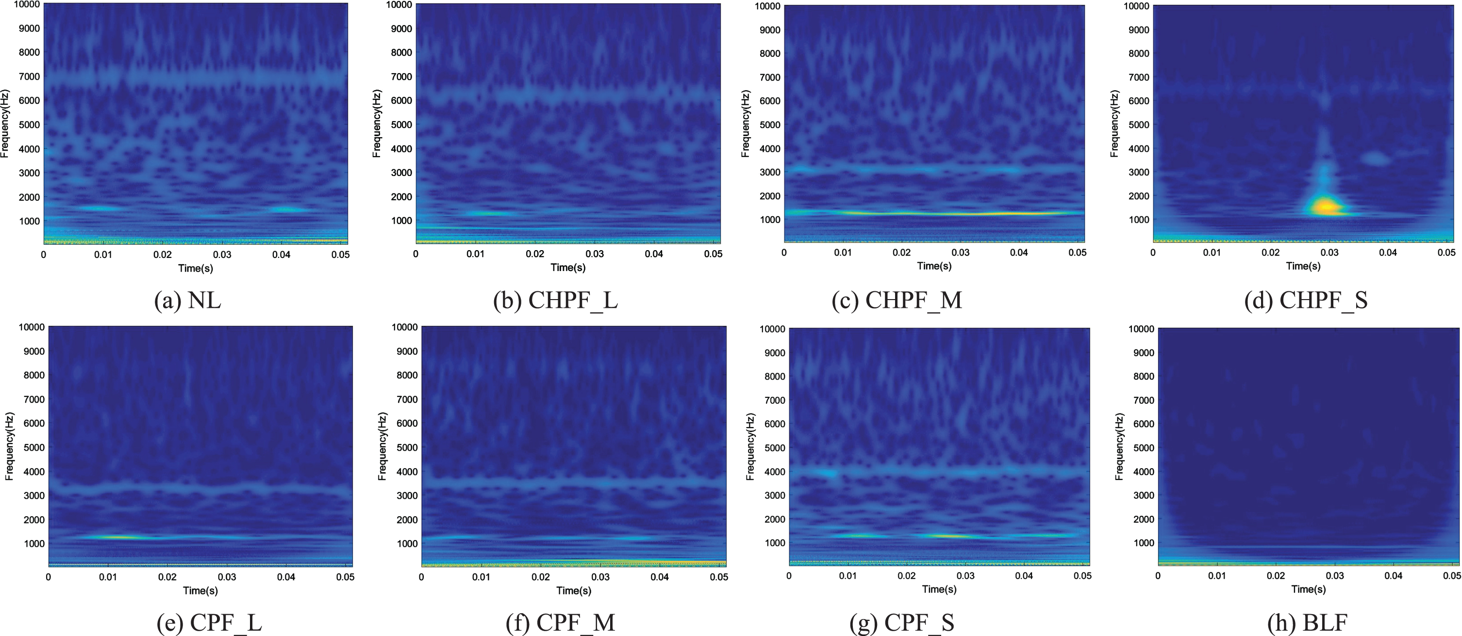
Time–frequency images of actual samples: (a) NL; (b) CHPF_L; (c) CHPF_M; (d) CHPF_S; (e) CPF_L; (f) CPF_M; (g) CPF_S; (h) BLF.

Fig. 6

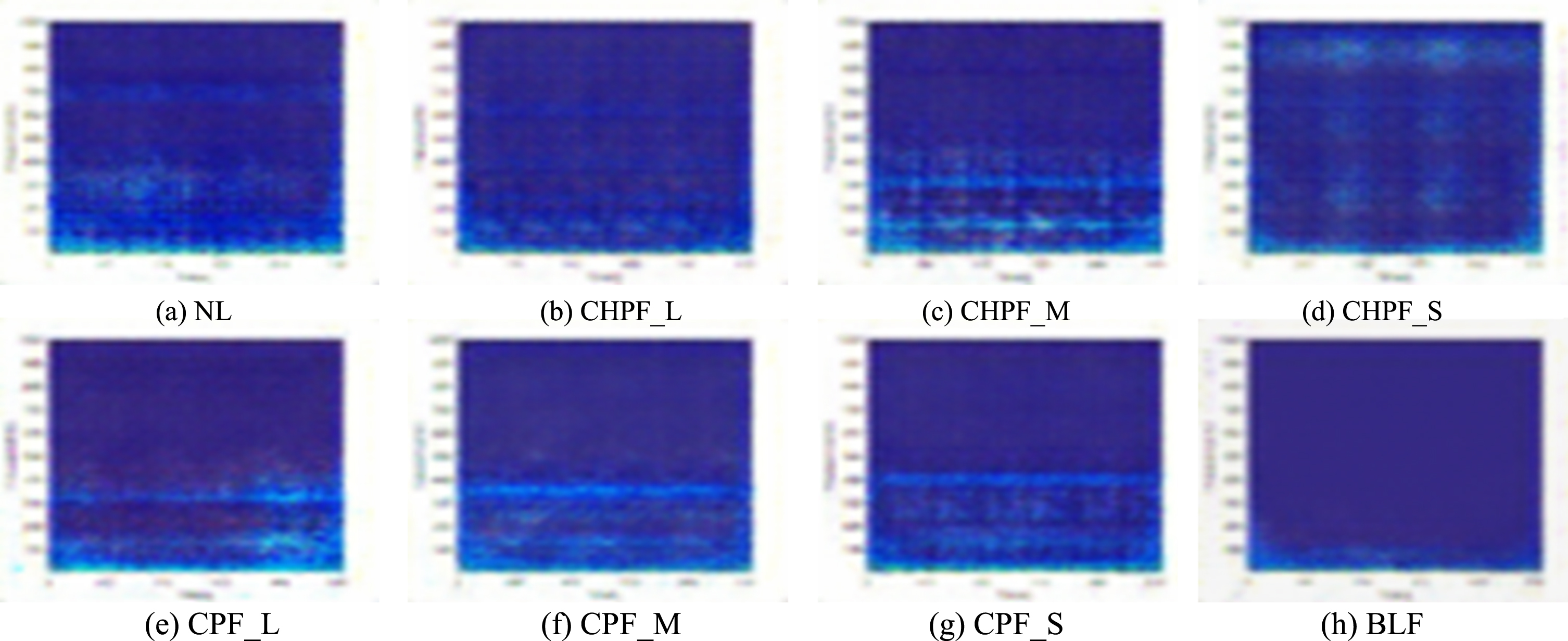
Time–frequency images of generated samples of IM_DCGAN model: (a) NL; (b) CHPF_L; (c) CHPF_M; (d) CHPF_S; (e) CPF_L; (f) CPF_M; (g) CPF_S; (h) BLF.

Three models—GAN, DCGAN, and IM_DCGAN—are trained; the loss curves for the generators and discriminators are presented in Fig. 7. Fig. 7(a) and Fig. 7(b) represent the change in the loss function of the generator and discriminator, respectively. The horizontal axis represents the number of iterations and the vertical axis represents the loss value. For the GAN model, the generator loss fluctuates significantly and the discriminator loss quickly converges to zero with an increase in the number of iterations, indicating that the GAN model cannot provide a reliable path to continuously update the generator gradient, eventually resulting in disappearance. For the DCGAN model, two types of losses fluctuate considerably before the 250th iteration; the model tends to be stable after the 250th iteration. Compared with the DCGAN model, the IM_DCGAN shows a small fluctuation in loss and converges rapidly. After nearly 1000 iterations, the loss of IM_DCGAN is less than that of DCGAN. The variance index is used to measure the fluctuations in loss of the discriminator, as shown in Table 6. A smaller variance results in a smaller data fluctuation and more stable model training.

Fig. 7

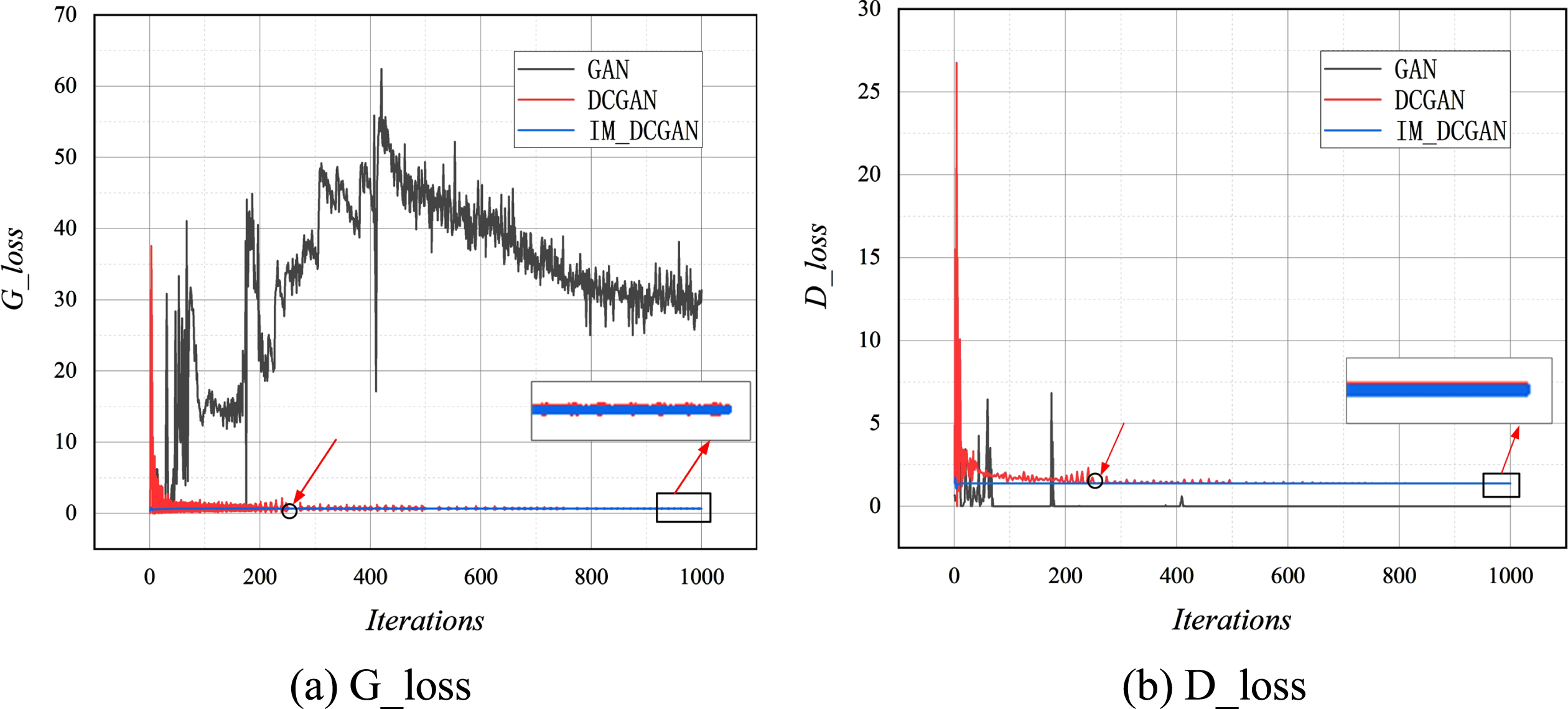
Comparison of training losses.

Table 6

Comparison of variance values

Network	GAN	DCGAN	IM_DCGAN
D (σ²)	0.28151	1.22497	0.00032

As shown in Table 6, the ratio of the variance of IM_DCGAN model to the variance of DCGAN model is less than 1% of the variance of DCGAN. which indicates that the IM_DCGAN model training is more stable and further proves that this study is effective for the improved method of the DCGAN.

The lack of quantitative evaluation criteria makes it difficult to reasonably evaluate the image generation quality of the GAN model [25]. Thus, this study combines appropriate evaluation indices: the inception score (IS) [26], Fréchet inception distance score (FID) [27, 28], peak signal to noise ratio (PSNR) [29], and structural similarity (SSIM) [30, 31]. The IS measures the clarity of images, and it is a pre-training Inception Net-V3 [32] network based on Google. A higher value indicates better image clarity. FID is improved on the basis of the IS, and it calculates the distance of feature vectors between actual images and generated images. A smaller value indicates that the image features are more similar. The unit of PSNR is dB, and it ranges from 20 to 40 dB; the SSIM ranges from 0 to 1. Both indicators conform to a common rule, i.e., a higher value indicates weaker distortion and more similarity between the images. The results of the image quality assessment are shown in Table 7.

Table 7

Results of image quality evaluation

Model	IS	FID	PSNR	SSIM
GAN	1.0342	247.93	13.3853	0.2546
DCGAN	1.0604	74.043	27.7897	0.9688
IM_DCGAN	1.0613	51.88	31.8961	0.9790

As shown in Table 7, the values of IS, PSNR, and SSIM for the images generated by the IM_DCGAN model are higher than those for the images generated by the DCGAN and GAN; moreover, the value of FID is the smallest. These results meet the quality assessment requirements, indicating that the generated images of the IM_DCGAN model are of good quality and diversity. It is impossible to effectively verify the influence of the generated images on the classification accuracy of the diagnosis model, because the image quality generated by the GAN is relatively low. Hence, only the IM_DCGAN and DCGAN models are used to generate image samples for experimental research. With different BDS requirements, four groups of imbalanced datasets for IM_DCGAN and DCGAN are constructed from the original A, B, C, and D datasets.

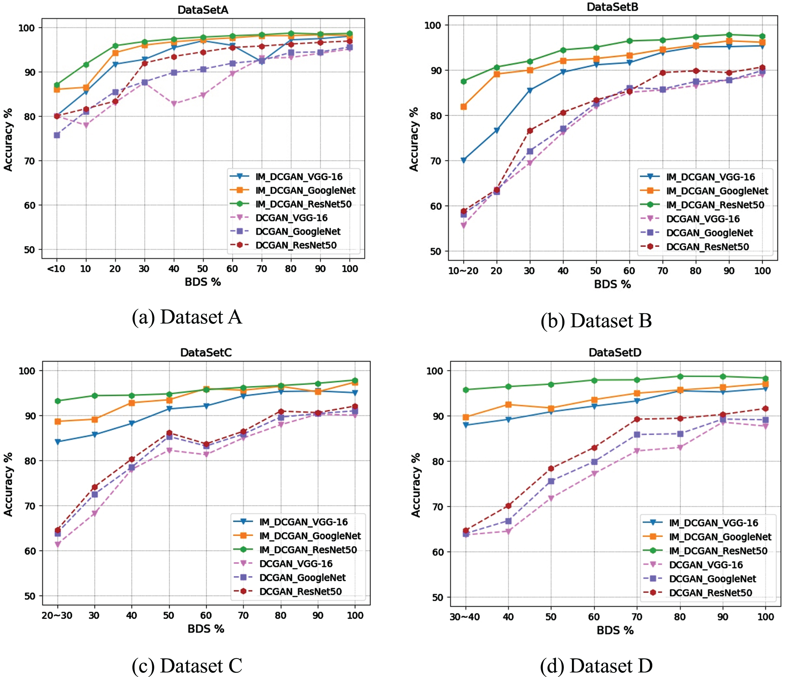
4.4 Fault classification and analyses

Three classical CNN models, including VGG-16 [33], GoogleNet [34], and ResNet [35], are constructed for comparative analyses with four groups of data, using different IM_DCGAN and DCGAN balance degrees as the input. Table 8(a) and Table 8(b) demonstrate the classification accuracy of IM_DCGAN and DCGAN over the imbalanced datasets, respectively; the comparative results are presented in Fig. 8.

Table 8(a)
Classification results of IM_DCGAN for each dataset under different BDS values

Dataset A Model <10% 10% 20% 30% 40% 50% 60% 70% 80% 90% 100%

VGG-16 80.00 85.42 91.67 92.74 95.39 96.94 95.91 92.25 97.16 97.43 97.97

GoogleNet 86.00 86.46 94.27 95.97 96.71 97.22 97.60 98.08 98.11 98.29 98.13

ResNet50 87.00 91.67 95.83 96.77 97.37 97.78 98.08 98.31 98.67 98.46 98.59

Dataset B Model / 10∼20% 20% 30% 40% 50% 60% 70% 80% 90% 100%

VGG-16 / 70.00 76.56 85.48 89.47 91.11 91.59 93.86 95.08 95.12 95.31

GoogleNet / 81.88 89.06 89.92 92.11 92.50 93.27 94.49 95.45 96.40 96.09

ResNet50 / 87.50 90.62 91.94 94.41 95.00 96.39 96.61 97.35 97.77 97.50

Dataset C Model / / 20∼30% 30% 40% 50% 60% 70% 80% 90% 100%

VGG-16 / / 84.09 85.66 88.16 91.39 92.07 94.28 95.27 95.38 95.00

GoogleNet / / 88.64 89.11 92.78 93.43 95.91 95.55 96.40 95.21 97.34

ResNet50 / / 93.18 94.35 94.44 94.74 95.67 96.19 96.59 97.09 97.81

Dataset D Model / / / 30∼40% 40% 50% 60% 70% 80% 90% 100%

VGG-16 / / / 87.86 89.14 90.83 92.07 93.22 95.45 95.21 95.94

GoogleNet / / / 89.64 92.42 91.67 93.51 94.92 95.64 96.23 97.03

ResNet50 / / / 95.71 96.38 96.94 97.84 97.88 98.67 98.63 98.28

Dataset A	Model	<10%	10%	20%	30%	40%	50%	60%	70%	80%	90%	100%
	VGG-16	80.00	85.42	91.67	92.74	95.39	96.94	95.91	92.25	97.16	97.43	97.97
	GoogleNet	86.00	86.46	94.27	95.97	96.71	97.22	97.60	98.08	98.11	98.29	98.13
	ResNet50	87.00	91.67	95.83	96.77	97.37	97.78	98.08	98.31	98.67	98.46	98.59
Dataset B	Model	/	10∼20%	20%	30%	40%	50%	60%	70%	80%	90%	100%
	VGG-16	/	70.00	76.56	85.48	89.47	91.11	91.59	93.86	95.08	95.12	95.31
	GoogleNet	/	81.88	89.06	89.92	92.11	92.50	93.27	94.49	95.45	96.40	96.09
	ResNet50	/	87.50	90.62	91.94	94.41	95.00	96.39	96.61	97.35	97.77	97.50
Dataset C	Model	/	/	20∼30%	30%	40%	50%	60%	70%	80%	90%	100%
	VGG-16	/	/	84.09	85.66	88.16	91.39	92.07	94.28	95.27	95.38	95.00
	GoogleNet	/	/	88.64	89.11	92.78	93.43	95.91	95.55	96.40	95.21	97.34
	ResNet50	/	/	93.18	94.35	94.44	94.74	95.67	96.19	96.59	97.09	97.81
Dataset D	Model	/	/	/	30∼40%	40%	50%	60%	70%	80%	90%	100%
	VGG-16	/	/	/	87.86	89.14	90.83	92.07	93.22	95.45	95.21	95.94
	GoogleNet	/	/	/	89.64	92.42	91.67	93.51	94.92	95.64	96.23	97.03
	ResNet50	/	/	/	95.71	96.38	96.94	97.84	97.88	98.67	98.63	98.28

Fig. 8

Comparison of the classification performance of IM_DCGAN and DCGAN for different BDS values.

As shown in Fig. 8, the accuracy of the CNN models is improved significantly with an increase in the BDS index. On comparing the images generated by the IM_DCGAN and DCGAN models, it is observed that the image classification accuracy achieved by adding the IM_DCGAN model to the original sample is greater than that of the DCGAN. The classification accuracies of VGG-16, GoogleNet, and ResNet50 were 96.41%, 97.19%, and 99.22%, respectively, for the original balanced dataset. The classification results of IM_DCGAN were more similar to the actual balanced datasets than those of the DCGAN, further indicating that the image quality achieved by the IM_DCGAN model is better and more diverse. To elucidate the influence of sample balance on the classification accuracy, images produced by the IM_DCGAN model are analyzed.

Dataset A has the fewest fault samples; the proportion of fault samples is less than 10%. However, the classification accuracy of Dataset A is greater than 80% in Table 8(a), which is not consistent with the large amount of data required for training a deep learning model. Thus, the authenticity of this classification accuracy cannot be guaranteed. Using the ResNet50 model as an example, the classification results of eight states with different BDS index values are shown in Table 9. When the ratio of fault samples to normal samples is less than 10%, the accuracy of NL and BLF is 100%, the accuracy of CHPF_M is 75%, and the accuracy of other fault classifications is 0. When the BDS is increased to 20%, the classification accuracy of the eight states exceeds 80%, as shown in Fig. 9(a). The classification results of the eight states for datasets B, C, and D are shown in Fig. 9(b), Fig. 9(c), and Fig. 9(d), respectively. When the proportion of fault samples is less than 30%, the classification accuracy for individual faults is significantly low and missed diagnoses may occur; when the BDS exceeds 30%, the classification accuracy of the eight states improves with an increase in the BDS value.

Table 8(b)

Classification results of DCGAN for each dataset under different BDS values

Dataset A	Model	<10%	10%	20%	30%	40%	50%	60%	70%	80%	90%	100%
	VGG-16	80.00	77.94	82.99	87.50	82.73	84.72	89.54	93.01	93.18	94.14	95.08
	GoogleNet	75.74	80.99	85.48	87.70	89.80	90.56	91.89	92.53	94.32	94.43	95.55
	ResNet50	80.00	81.62	83.33	91.94	93.42	94.44	95.43	95.76	96.21	96.58	96.88
Dataset B	Model	/	10∼20%	20%	30%	40%	50%	60%	70%	80%	90%	100%
	VGG-16	/	55.63	63.54	69.35	76.15	81.87	85.04	85.54	86.51	87.84	88.91
	GoogleNet	/	58.13	63.02	72.08	77.06	82.64	86.06	85.75	87.41	87.71	89.84
	ResNet50	/	58.75	63.54	76.61	80.59	83.33	85.34	89.41	89.77	89.38	90.62
Dataset C	Model	/	/	20∼30%	30%	40%	50%	60%	70%	80%	90%	100%
	VGG-16	/	/	61.36	68.15	77.96	82.22	81.25	84.96	87.88	90.24	90.00
	GoogleNet	/	/	63.86	72.48	78.45	85.28	83.17	85.81	89.58	90.37	90.98
	ResNet50	/	/	64.55	74.09	80.26	86.11	83.65	86.44	90.91	90.58	92.03
Dataset D	Model	/	/	/	30∼40%	40%	50%	60%	70%	80%	90%	100%
	VGG-16	/	/	/	63.66	64.47	71.79	77.16	82.20	82.95	88.53	87.66
	GoogleNet	/	/	/	63.93	66.78	75.56	79.81	85.81	85.98	89.21	89.06
	ResNet50	/	/	/	64.64	70.07	78.33	82.93	89.19	89.39	90.24	91.56

Table 9

Classification results of ResNet50 for different BDS values on Dataset A

Dataset A	<10%	10%	20%	30%	40%	50%	60%	70%	80%	90%	100%
BLF	100.00	100.00	100.00	100.00	100.00	100.00	100.00	100.00	100.00	100.00	100.00
CHPF_L	0	87.50	87.50	91.67	93.75	95.00	95.83	96.43	98.44	97.22	97.50
CHPF_M	75.00	87.50	100.00	95.30	96.88	97.50	100.00	98.21	98.44	97.22	98.75
CHPF_S	0	62.50	81.25	87.50	90.62	92.50	93.75	94.64	95.31	95.83	96.25
CPF_L	0	87.50	100.00	100.00	100.00	100.00	97.92	100.00	100.00	100.00	98.75
CPF_M	0	100.00	100.00	100.00	100.00	100.00	100.00	100.00	100.00	100.00	100.00
CPF_S	0	75.00	87.50	91.67	93.75	95.00	95.83	96.43	96.88	97.22	97.50
NL	100.00	100.00	98.75	100.00	100.00	100.00	100.00	100.00	100.00	100.00	100.00

Fig. 9

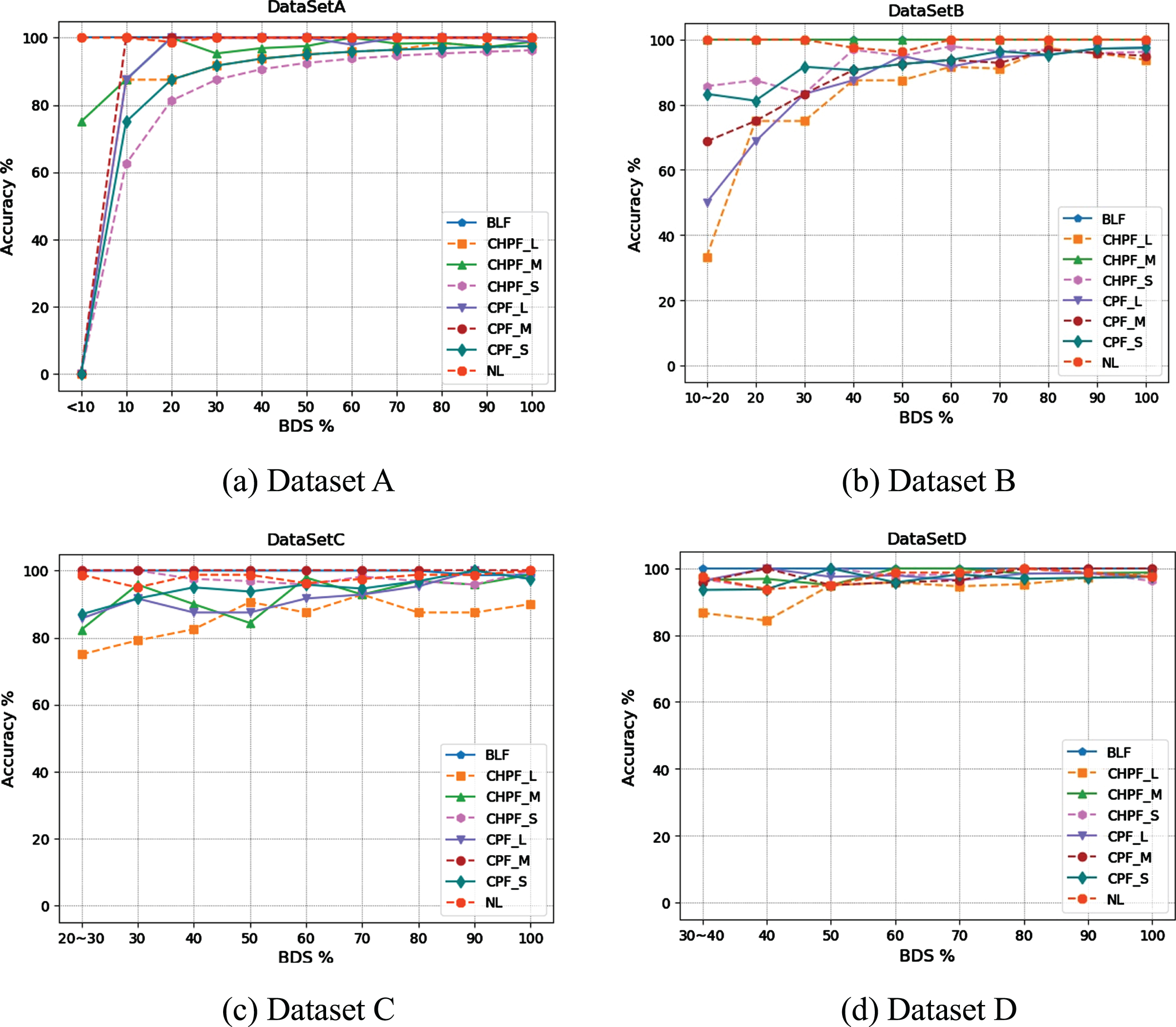
Classification results of ResNet50 for different BDS values.

Figure 10 shows the distribution of the accuracies of the VGG-16, GoogleNet, and ResNet50 models with respect to the datasets with different balance degrees. The accuracy of each model exceeds 95% and tends to remain stable when the BDS is 80~100%. This indicates that, when the number of samples is sufficient, the classification model has less impact on the classification results, which mainly depend on the quality of the generated image and the number of added samples.

Fig. 10

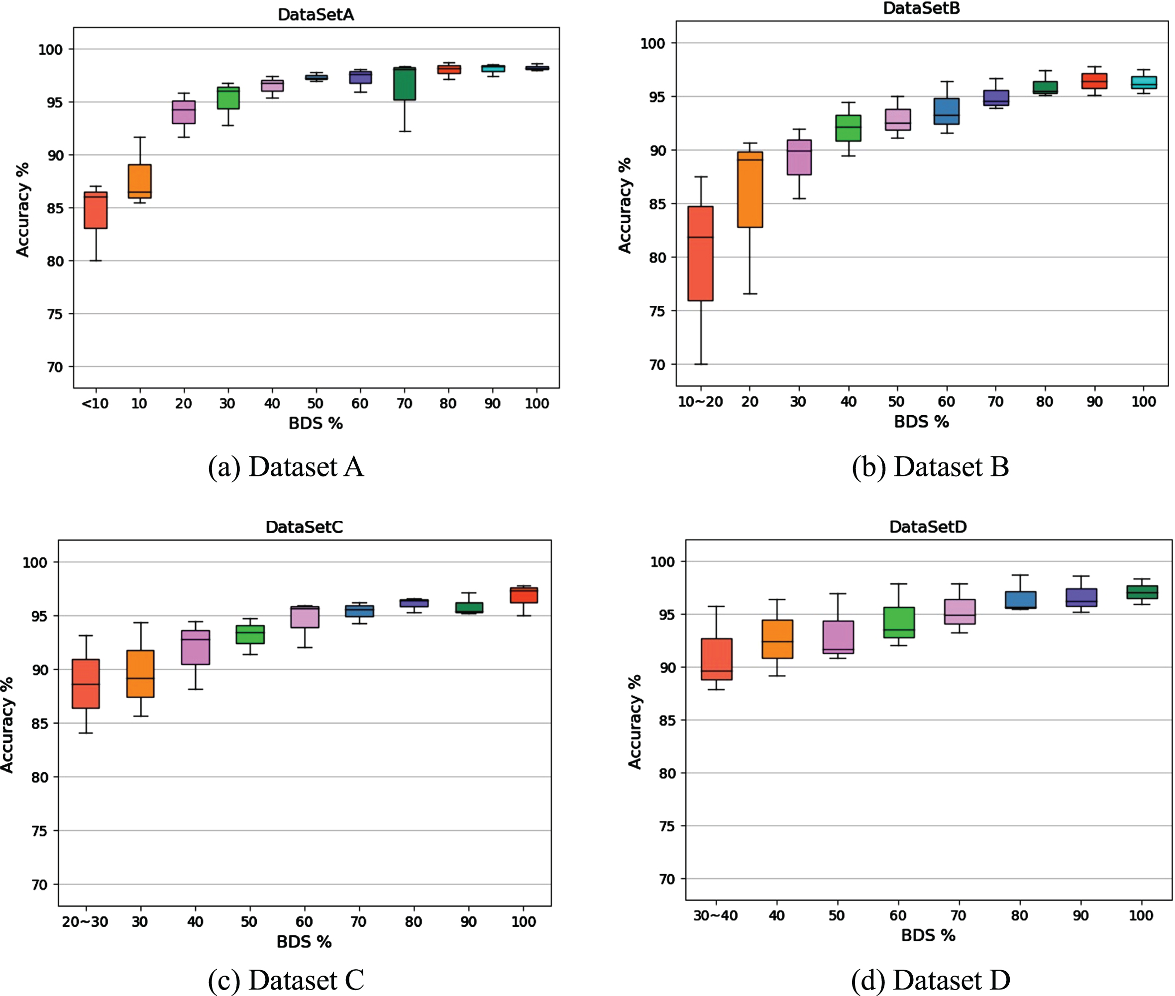
Accuracy range of each model for different BDS values.

Based on the experiment and results, findings are as follows: a) when the proportion of fault samples is less than 30%, it is preferable to avoid training the model, because it would often fail to detect minority samples or the classification accuracy for certain types of faults is low, leading to missed diagnoses of faults. b) When the BDS is 30~80%, the classification accuracy increases with an increase in the BDS value. In this case, it is suggested that the number of fault samples be increased to improve the classification accuracy. c) When the BDS is 80~100%, the classification accuracy exceeds 95% and tends to remain stable; in this case, excessive samples should not be added for fault classification, which can increase operation costs.

5 Conclusion

In order to ensure the stable and reliable operation of equipment and reduce equipment failures, an improved DCGAN was proposed to enhance the imbalanced sample data in view of the imbalanced sampling of mechanical equipment. As impacted by the unstable training and slow convergence of the DCGAN model, the spectral normalization was conducted for each convolutional layer in discriminant D, so the optimized model could effectively prevent excessively sharp alterations in the parameters of discriminant D and improve the model to be more stable. After the variance of the lost data was calculated, the improved DCGAN in this study was further proven to be more effective than the original model. Subsequently, four indexes, which were FID, IS, PSNR and SSIM, were adopted to assess the quality of the generated images quantitatively. The different index values of the IM_DCGAN were more consistent with the quality assessment standard range, which demonstrated that the generated images exhibited the better quality and the stronger diversity. In this study, the BDS index was proposed to form several sets of samples with different balance degrees were constructed and input into the CNN models for fault classification. Datasets with different balance degrees were analyzed and the rules were summarized, which are expected to serve as a reference for the macro analysis of fault diagnosis in the future. In future research, the generation model and the diagnosis model will be integrated to realize end-to-end application (i.e., from sample generation to fault diagnosis) in order to reduce the complexity of fault diagnoses and improve efficiency with imbalanced input conditions. Moreover, the assessment system of the quality of generated images should be urgently improved, and a standardized and universal scientific assessment system is required.

Footnotes

Acknowledgments

This work was supported by National Natural Science Foundation of China (No. 51674277) and the Strategic Cooperation Technology Projects of CNPC and CUPB (ZLZX2020-05-02).

References

Wang

Z.X.

, FLOWGAN: Research on key technology of encrypted traffic identification based on generative adversarial network, Master Dissertation, Nanjing University Of Posts And Telecommunications, (2020).

Chawlan

, Bowyer

K.W.

and Hall

O.L.

, SMOTE: synthetic minority over-sampling technique, Journal of Artificial Intelligence Research (2002), 321–357.

Xie

M.Y.

, Methods for Reciprocating Compressor Multi-Fault Identification under Imbalanced Datasets, Master Dissertation, China University of Petroleum (Beijing), (2018).

Xiang

H.Y.

and Yang

, Survey on Imbalanced Data Mining Methods, Computer Engineering and Applications (2019), 1–16.

Zhang

X.F.

and Gang

, Data augmentation method based on generative adversarial network, Computer Systems and Applications (2019), 201–206.

Lan

, Shen

H.F.

and Wang

, Dataset enhancement method based on improved deep convolutional generative adversarial networks, Journal of Computer Applications (2021), 1–11.

Mao

X.D.

, Li

and Xie

H.R.

, Least squares generative adversarial networks, Proceedings of IEEE International Conference on Computer Vision (ICCV), (2017).

Goodfellow

I.J.

, Pouget-Abadie

and Mirza

, Generative adversarial nets, Conference and Workshop on Neural Information Processing Systems (2014), 2672–2680.

Luc

, Couprie

and Chintala

, Semantic segmentation using adversarial networks, Proceedings of the 30th Conference on Neural Information Processing Systems (2016).

10.

Zhou

, Research on Image Generation Method Based on Deep Learning, Master Dissertation, Lanzhou University, (2019).

11.

Radford

, Metz

and Chintala

, Unsupervised representation learning with deep convolutional generative adversarial networks, International Conference on Learning Representations (2016), 1–16.

12.

Arjovsky

, Chintala

and Bottou

, Wasserstein generative adversarial networks, Proceedings of the 34th International Conference on Machine Learning Princeton, (2017), 298321.

13.

Gulrajani

, Ahmed

and Arjovsky

, Improved training of Wasserstein GANs[J], ar Xiv:1704.00028, (2017).

14.

Liang

J.J.

, Wei

J.J.

and Jiang

Z.F.

, Generative Adversarial Networks GAN Overview, Journal of Frontiers of Computer Science and Technology (2020), 1–17.

15.

Zhang

Z.H.

, Zeng

Y.B.

and Lu

, Spectral bounding: Strictlysatisfying the 1-Lipschitz property for generative adversarialnetworks[J], Pattern Recognition 105 2020, 1–10.

16.

Tan

H.W.

, Zhou

L.Y.

and Wang

G.D.

, Instability analysis for generative adversarial networks and its solving techniques, Scientia Sinica(Informationis) (2021), 1–16.

17.

Miyato

, Kataoka

and Koyama

, Spectral Normalization for Generative Adversarial Networks[EB/OL], https://arxiv.org/pdf/1802.05957.pdf, (2020).

18.

N.N.

and Zheng

, Multi-loss ensemble and spectral normalization for image super-resolution, Application Research of Computers (2020), 2531–2535.

19.

Z.P.

, Guo

L.L.

and Zhu

M.C.

, Improved image registration using feature points combined with image entropy, Infrared and Laser Engineering (2013), 2846–2852.

20.

Scaman

and Virmaux

, Lipschitz regularity of deep neural networks: Analysis and efficient estimation, Proceedings of the 32nd Conference on Neural Information Processing Systems (2018), 3835–3844.

21.

Zhang

Z.X.

, Yuan

J.Q.

and Guo

H.L.

, Multi-discriminator Co-operation Framework: Spectral Normalized Generative Adversarial Networks for High Quality Generated Images, Journal of Chinese Computer Systems (2021), 201–207.

22.

Gan

, Shen

H.F.

and Wang

, Simulation Method of Target SAR Image Based on Spectral Normalization Generative Adversarial Network, Computer and Modernization (2021), 1–11.

23.

, Research on heterogeneous features fusion and online imbalance classification for bearing fault diagnosis, Master Dissertation, Henan Normal University, (2017).

24.

Zhong

S.S.

, Li

and Zhang

Y.J.

, Fault diagnosis of civil aero-engine driven by unbalanced amples based on DBN, Journal of Aerospace Power (2019), 708–716.

25.

Borji

, Pros and cons of GAN evaluation measures, Computer Vision and Image Understanding (2019), 41–65.

26.

Salimans

, Goodfellow

and Zaremba

, Improved techniques for training GANs, Advances in Neural Information Processing Systems, Curran Associates (2016), 2234–2242.

27.

Tran

N.T.

, Tran

V.H.

and Nguyen

N.B.

, On Data Augmentation for GAN Training, IEEE Transactions on Image Processing (2021), 1882–1897.

28.

Zhang

, Xu

G.H.

and Han

Z.Z.

, Data Augmentation for Motor Imagery Signal Classification Based on a Hybrid Neural Network, Sensors (2020), 1–20.

29.

Huynh-Thu

and Ghanbari

, Scope of validity of PSNR in image/video quality assessment, Electronics Letters (2008), 800–801.

30.

Wang

, Bovik

A.C.

and Sheikh

H.R.

, Image quality assessment: from error visibility to structural similarity, IEEE Transactions on Image Processing (2004), 600–612.

31.

Zhong

G.Q.

, Gao

and Liu

Y.B.

, Generative adversarial networks with decoder–encoder output noises, Neural Networks (2020), 19–28.

32.

Szegedy

, Vanhoucke

and Ioffe

, Rethinking the Inception Architecture for Computer Vision, 2016 IEEE Conference on Computer Vision and Pattern Recognition (CVPR) (2016), 2818–2826.

33.

Russakovsky

, Deng

and Su

, ImageNet Large Scale Visual Recognition Challenge, International Journal of Computer Vision (2015), 211–252.

34.

Szegedy

, Liu

and Jia

, Going Deeper with Convolutions, 2015 IEEE Conference on Computer Vision and Pattern Recognition (CVPR). USA: IEEE Computer Society, (2015), 1–9.

35.

, Zhang

and Ren

, Deep Residual Learning for Image Recognition, 2016 IEEE Conference on Computer Vision and Pattern Recognition (CVPR), USA: IEEE Computer Society, (2016), 770–778.

Imbalanced data enhancement method based on improved DCGAN and its application

Abstract

Keywords

1 Introduction

2 Theoretical background

2.1 Wavelet transform (WT)

3.1 Theoretical analysis of improved DCGAN model

Table 3 Abnormal crosshead clearance parameters State types Fault degree of crosshead clearance Original copy Marginal wear Moderate wear Severe wear Crosshead pin diameter 15.80 mm 15.70 mm 15.60 mm 15.50 mm Clearance value 0 mm 0.10 mm 0.20 mm 0.30 mm

4.3 Data enhancement

Footnotes

Acknowledgments

References

Table 3
Abnormal crosshead clearance parameters

State types Fault degree of crosshead clearance

Original copy Marginal wear Moderate wear Severe wear

Crosshead pin diameter 15.80 mm 15.70 mm 15.60 mm 15.50 mm

Clearance value 0 mm 0.10 mm 0.20 mm 0.30 mm