A study of an EOQ model with public-screened discounted items under cloudy fuzzy demand rate

Abstract

This article deals with an economic order quantity inventory model of imperfect items under non-random uncertain demand. Here we consider the customers screen the imperfect items during the selling period. After a certain period of time, the imperfect items are sold at a discounted price. We split the model into three cases, assuming that the demand rate increases, decreases, and is constant in the discount period. Firstly, we solve the crisp model, and then the model is converted into a fuzzy environment. Here we consider the dense fuzzy, parabolic fuzzy, degree of fuzziness and cloudy fuzzy for a comparative study. The basic novelty of this paper is that a computer-based algorithm and flow chart have been given for the solution of the proposed model. Finally, sensitivity analysis and graphical illustration have been given to check the validity of the model.

Keywords

Imperfect inventory dense fuzzy number parabolic fuzzy number cloudy fuzzy number degree of fuzziness optimization

1 Introduction

In 1965 Zadeh [8] introduced us to an uncertain world. He claimed that except for some universal truth, there is uncertainty behind every fact. He handled this uncertainty by using the membership value of each element in a set. This type of set is called fuzzy set. After that, Bellman and Zadeh [14] used the fuzzy set concept in operations research decision-making. After that, Atanassov [7] define intuitionistic fuzzy set, which contains not only membership value but also non-membership value of each element in a set. Baez-Sanchez et al. [3] developed a mathematical formalization to define polygonal fuzzy numbers with an extension of fuzzy sets. De and Beg [26] introduced the concept of dense fuzzy set by incorporating learning experiences in fuzzy set. They considered each member of a fuzzy set as a sequence of functions that converge to a crisp number for n→ ∞. They also define a new defuzzification method of triangular dense fuzzy set. Also, De and Beg [25] described the dense fuzzy Neutrosophic set. De and Mahata [24] introduced the concept of cloudy fuzzy number, which converge to a crisp number after infinite times. They used this concept to optimize a backorder economic order quantity (EOQ) model with uncertain demand rate. We know every inventory decision-maker used some strategies to optimize the inventory profit. Keeping this in mind, De [31] introduced the dense fuzzy lock set concept, which is much more helpful for the decision-maker to manage the inventory control problems. Faritha and Priya [2] defined parabolic fuzzy number for optimizing a backorder EOQ model using nearest interval approximation. Then Garg and Ansha [5] defined some arithmetic operations over generalized parabolic fuzzy numbers with its applications. Maity et al. [18] introduced the concept of non-linear heptagonal dense fuzzy set with an application in inventory problems. Maity et al. [20] also defined cloud-type non-linear intuitionistic dense fuzzy set with symmetry and asymmetry cases. De [30] gave a new concept over the degree of fuzziness and its application in decision-making problems. From the above literature review of fuzzy numbers, we see that every researcher considered one type of fuzzy number with an application. None of them didn’t give a comparative study to examine which fuzzy number is more profitable for inventory management. This model provided a comparative study among dense fuzzy, cloudy fuzzy, parabolic fuzzy and degree of fuzziness over the inventory profit function.

Harris [4] first developed the classical inventory model. After that, several researchers produced many research articles on inventory problems. All of them considered the demand rate as a deterministic one. First time Karlin [15] introduced fuzziness in one stage inventory problems. Nowadays, modern researchers are showing their interest in solving inventory problems in fuzzy environments. De [29] developed an EOQ model under daytime non-random uncertain demand. Das et al. [12] solved an EOQ model using a step order fuzzy approach. He considered daytime uncertain demand where demand in the backorder period depends on time. De et al. [28] studied an EOQ model where demand depends on selling price and promotional efforts. The model has been optimized using the intuitionistic fuzzy technique. Kazemi et al. [11] solved an EOQ model for imperfect quality items by considering the learning effect on some fuzzy parameters. In 2016, De and Sana [27] developed an economic production quantity (EPQ) model with variable lead time and stochastic demand. They considered all parameters the intuitionistic fuzzy number and used the intuitionistic fuzzy aggregation Bonferroni mean for defuzzified the model. Karmakar et al. [16, 17] considered an EPQ model and used the dense fuzzy lock set concept to reduce pollution by reusing waste items of sponge iron industry. Maity et al. [19] developed an EOQ model with dense fuzzy demand rate where two decision-makers make a single decision to optimize the model. Maity et al. [21] studied an EOQ model under daytime uncertain demand rate. They made a computer-based algorithm and flowchart to optimize the model by updating key vectors automatically. De and Mahata [22] considered an EOQ model of imperfect-quality items with considerable discounts. They optimized the model using cloudy fuzzy numbers. Liang and Wang [13] presented an integrated decision support model for the customers to buy their desired products online. Traditionally, De and Mahata [23] developed an EOQ model of imperfect quality items where the retailer first screened the items. Then the imperfect items are sold separately at a discount. Several researchers (Khan et al. [9], Lin and Chen [32], Naimi and Tahavori [10], Sofiana and Rosvidi [1], Wangsa and Wee [6] and Zhou et al. [33]) studied over imperfect quality items. Still, none of the researchers has considered the situations where the customers screened the items, although it happens in reality in most cases. They did not also consider all three possible cases of the demand rate in the discount period, which is included in this paper.

In the present study, we consider the low demanded items screened by the customers during the sales. After a certain period, the low demanded items are sold at a discount. Here we have considered three possibilities of demand in the discount period - (i) demand increases exponentially, (ii) demand decreases exponentially, (iii) demand remains same as previous. We have taken a crisp solution first. Then we have solved it in cloudy fuzzy, dense fuzzy, parabolic fuzzy and degree of fuzziness environment. Then we have provided a case study with sensitivity analysis and graphical illustrations to justify our proposed model. The numerical result is determined by LINGO 16.0 software. A computer-based algorithm and flowchart of the proposed method are provided for easy understanding.

The remaining part of this paper is arranged in the following way. In Section 2, we have added some preliminary definitions of different types of fuzzy numbers. The crisp mathematical model has been developed in Section 3. Section 4 contain the cloudy fuzzy model of three different cases. In Section 5, we have discussed other fuzzy models (dense fuzzy model and parabolic fuzzy model). A solution algorithm and flowchart of the proposed model are given in Section 6. A case study of the proposed model is discussed in Section 7. Section 8 contain the graphical illustration of the numerical result and Section 9 contain some advantages and disadvantages of our proposed model. Finally, a brief conclusion has been given in Section 10.

2 Preliminaries

In this section, the preliminary concept of different types of fuzzy numbers are discussed.

Definition 1. Dense Fuzzy Number [26] Let $\tilde{X} = 〈 a_{n}, a_{n - 1}, \dots, a_{1}, a, a_{1}^{'}, \dots, a_{n - 1}^{'}, a_{n}^{'} 〉$ be a fuzzy number containing 2n + 1 components and $a_{i} = {af}_{i}, a_{i}^{'} = {ag}_{i}, fori = 1, 2, \dots, n$ where f_i and g_i are sequence of functions. If the components f_i and g_i are converges to 1 for n→ ∞ then the fuzzy number $\tilde{X}$ is also converge to a. Then the fuzzy number $\tilde{X}$ is called as dense fuzzy number.

Definition 2. Triangular Dense Fuzzy Number (TDFN) [26] If $\tilde{B} = 〈 b (1 - \frac{ρ}{1 + n}), b, b (1 + \frac{σ}{1 + n}) 〉$ is a triangular dense fuzzy number then its membership function of $\tilde{B}$ is given by $μ (y, n) = {\begin{matrix} \frac{y - b (1 - \frac{ρ}{1 + n})}{\frac{b ρ}{1 + n}}, & for b (1 - \frac{ρ}{1 + n}) ⩽ y ⩽ b \\ 1, & fory = b \\ \frac{b (1 + \frac{σ}{1 + n}) - y}{\frac{b σ}{1 + n}}, & for b ⩽ y ⩽ b (1 + \frac{σ}{1 + n}) \\ 0, & for elswhere \end{matrix}$

Let us consider b = 100, ρ = 0.4, σ = 0.4. For this value the TDFN is shown in Fig. 1.

Fig. 1

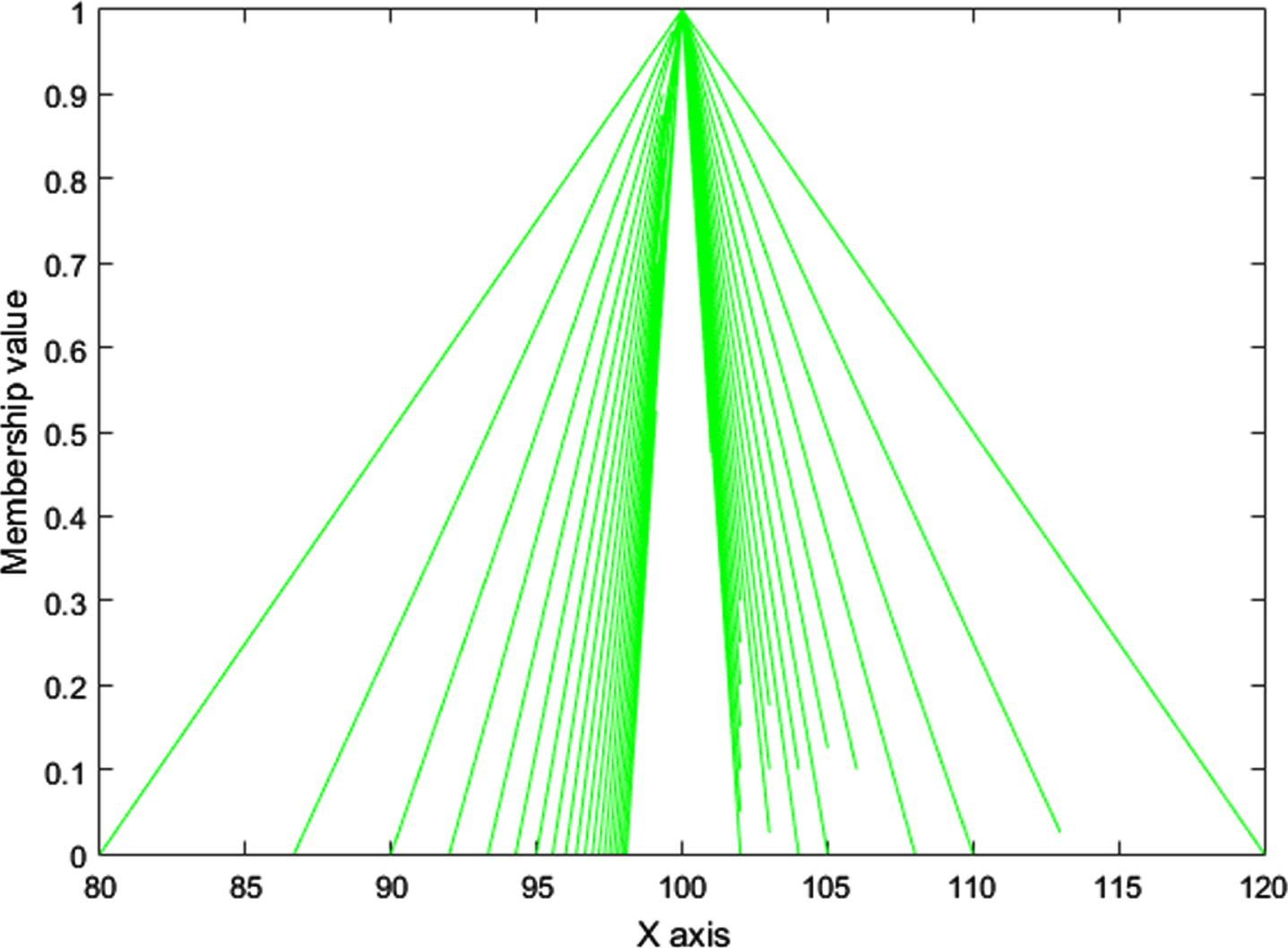
Membership function of TDFN.

Defuzzification formula [26] If $μ_{L}^{α} and μ_{R}^{α}$ are left and right α –cuts of the TDFN then the defuzzified value is given by $I (\tilde{B}) = \frac{1}{2 N} \sum_{n = 1}^{N} \int_{α = 0}^{1} (μ_{L}^{B} + μ_{R}^{B}) d α$ (1)

Definition 3. Parabolic fuzzy number (PFN) [5] The fuzzy number $\tilde{B} = 〈 b (1 - ρ), b, b (1 + σ) 〉$ is said to be a parabolic fuzzy number if its membership function is as follow $μ_{B} (y) = {\begin{matrix} {\frac{y - b (1 - ρ)}{b ρ}}^{2}, & for b (1 - ρ) ⩽ y ⩽ b \\ 1, & for y = b \\ {\frac{b (1 + σ) - y}{b σ}}^{2}, & for b ⩽ y ⩽ b (1 + σ) \\ 0, & for elswhere \end{matrix}$ (2)

New Defuzzification formula of PFN Let $\tilde{B} = 〈 b (1 - ρ), b, b (1 + σ) 〉$ be a PFN with the membership fction defined in (2). Then utilising the left and right α –cuts of the PFN we have defined the new defuzzified index as follows $I (\tilde{B}) = \frac{1}{2} \int_{α = 0}^{1} (μ_{L}^{B} + μ_{R}^{B}) d α$ (3) where $μ_{L}^{B} and μ_{R}^{B}$ are left and right α –cuts respectively.

Definition 4. Cloudy Fuzzy Number [24] Let $\tilde{X} = 〈 a_{n}, a_{n - 1}, \dots, a_{1}, a, a_{1}^{'}, \dots, a_{n - 1}^{'}, a_{n}^{'} 〉$ be fuzzy number containing 2n + 1 components. If the set itself converges to a crisp singleton set after an infinite time then the fuzzy number is called 2n+1 tuple cloudy fuzzy number.

Definition 5. Triangular Cloudy Fuzzy Number [24] Let $\tilde{B} = 〈 b (1 - \frac{ρ}{1 + t}), b, b (1 + \frac{σ}{1 + t}) 〉$ be a triangular fuzzy number. When t→ ∞ the fuzzy number converges to a crisp singleton set. So, $\tilde{B}$ is called cloudy triangular fuzzy number. Then its membership function is given by $μ (y, t) = {\begin{matrix} \frac{y - b (1 - \frac{ρ}{1 + t})}{\frac{b ρ}{1 + t}}, & for b (1 - \frac{ρ}{1 + t}) ⩽ y ⩽ b \\ 1, & for y = b \\ \frac{b (1 + \frac{σ}{1 + t}) - y}{\frac{b σ}{1 + t}}, & for b ⩽ y ⩽ b (1 + \frac{σ}{1 + t}) \\ 0, & for elswhere \end{matrix}$ (4)

Defuzzification formula of Cloudy fuzzy number [24] Let $μ_{L}^{α} and μ_{R}^{α}$ be left and right α –cuts of μ (y, t) respectively obtained from (4). Then the defuzzification formula is given by $I (\tilde{B}) = \frac{1}{2 T} \int_{α = 0}^{1} \int_{t = 0}^{T} {μ_{L}^{α} + μ_{R}^{α}} d α dt$ (5)

Definition 6. Polygonal fuzzy set [10] The fuzzy set with membership grades {f₁, f₂, … , f_n } and n + 1 vertex is called a polygonal fuzzy set of order n. The graph of a polygonal fuzzy set is shown in Fig. 2.

Fig. 2

Polygonal fuzzy set.

Definition 7. Degree of Fuzziness (DF) [30] Let $\tilde{B} = {b_{n}, \dots, b_{2}, b_{1}, b_{0}, b_{1}^{'}, b_{2}^{'}, \dots, b_{n}^{'}}$ be 2n+1 sided polygonal fuzzy set. Let the area of the polygon is denoted by and that of semi ellipse which covers the polygon is denoted by . Now the degree of fuzziness of the fuzzy set $\tilde{B}$ is denoted by D_f and defined by D_f =.

Degree of fuzziness of triangular fuzzy number [30] Let $\tilde{X} = 〈 b (1 - ρ), b, b (1 + σ) 〉$ be a triangular fuzzy number. Then $= \frac{b}{2} (ρ + σ)$ and $= \frac{b π}{4} (ρ + σ)$ . So, degree off fuzziness of triangular fuzzy number is given by $D_{f} = ifs-41-ifs210856-g009.jpg = 1 - \frac{2}{π}$ (6)

3 Crisp mathematical model

a. Notations and assumptions

The basic assumptions and notations of the model are

Assumptions

Replenishments are instantaneous

The time horizon is infinite

Shortages are not allowed, and lead time is zero

After receiving the products, customers buy their product according to their own choice. After a certain period of time the seller announces the discount for the low-quality products according to the customer’s view.

In addition, in the fuzzy model, we consider the demand rate assume dense fuzzy number, parabolic fuzzy number and cloudy fuzzy number.

Notations

q₁: Order quantity placed in order in starting of each cycle (decision variable)

q₂: The total amount of products sells with a considerable discount (decision variable)

t₁: Duration of selling without discount (decision variable)

t₂: Duration of selling with discount (t₁ > t₂) (decision variable)

d₁: Demand rate in time t₁

d₂: Demand rate in time t₂ (d₂ > d₁)

p: Purchasing price per unit item ($)

s: Selling price per unit item ($)

T: Cycle length (months)

c₁: Holding cost per unit quantity item per day ($)

c₃: Set up cost per cycle ($)

r: Discount rate in percentage

Z: Total profit per cycle ($)

b. Model formulation

Let the products are received instantaneously with purchasing price p per unit item, fixed ordering cost c₃ per cycle and holding cost c₁ per unit quantity item. Customers buy the products according to their own choice. After selling the good quality products in time t₁, the decision-maker will sell the remaining quantity q₂ with a considerable discount. The diagrammatic representation of the inventory model is shown in Fig. 3.

Fig. 3

Logistic diagram of the EOQ model.

From Fig. 3, total holding cost $= c_{1} [\frac{1}{2} t_{1} (q_{1} + q_{2}) + \frac{1}{2} t_{2} q_{2}]$ set up cost = c₃ and total purchasing price = pq₁

According to the above assumptions the total cost of the modified EOQ model is

TC = Holding cost+set up cost+total purchasing price $= c_{1} [\frac{1}{2} t_{1} (q_{1} + q_{2}) + \frac{1}{2} t_{2} q_{2}] + c_{3} + {pq}_{1}$

Total revenue per cycle TR = (q₁ - q₂) s + q₂ (1 - r) s

Total profit per cycle Z = TR - TC $= (q_{1} - q_{2}) s + q_{2} (1 - r) s - c_{1} [\frac{1}{2} t_{1} (q_{1} + q_{2}) + \frac{1}{2} t_{2} q_{2}] - c_{3} - {pq}_{1}$ $= d_{1} f_{1} + d_{2} f_{2} - c_{3}$ (7) $where {\begin{matrix} \begin{matrix} q_{1} = d_{1} t_{1} + d_{2} t_{2} \\ q_{2} = d_{2} t_{2} \end{matrix} \\ \begin{matrix} f_{1} = t_{1} s - \frac{c_{1} t_{1}^{2}}{2} - {pt}_{1} \\ f_{2} = t_{2} (1 - r) s - c_{1} t_{1} t_{2} - \frac{c_{1} t_{2}^{2}}{2} - {pt}_{2} \end{matrix} \end{matrix}$

Now, in reality, three cases can happen during the discount period. Due to discount demand can be increase or decrease or same as it is. These three cases are given below.

Case –(i): If d₂ = e^{t
₂}d₁ then the profit function becomes $Z = d_{1} φ - c_{3}$ (8) $where {\begin{matrix} \begin{matrix} φ = f_{1} + e^{t_{2}} f_{2} \\ q_{1} = d_{1} t_{1} + d_{2} t_{2} \end{matrix} \\ \begin{matrix} q_{2} = d_{2} t_{2} \\ f_{1} = t_{1} s - \frac{c_{1} t_{1}^{2}}{2} - {pt}_{1} \\ f_{2} = t_{2} (1 - r) s - c_{1} t_{1} t_{2} - \frac{c_{1} t_{2}^{2}}{2} - {pt}_{2} \end{matrix} \end{matrix}$ (9)

Case –(ii): If d₂ = e^-t₂d₁ then the profit function becomes $Z = d_{1} φ - c_{3}$ (10) $where {\begin{matrix} \begin{matrix} φ = f_{1} + e^{- t_{2}} f_{2} \\ q_{1} = d_{1} t_{1} + d_{2} t_{2} \end{matrix} \\ \begin{matrix} q_{2} = d_{2} t_{2} \\ f_{1} = t_{1} s - \frac{c_{1} t_{1}^{2}}{2} - {pt}_{1} \\ f_{2} = t_{2} (1 - r) s - c_{1} t_{1} t_{2} - \frac{c_{1} t_{2}^{2}}{2} - {pt}_{2} \end{matrix} \end{matrix}$ (11)

Case –(iii): If d₂ = d₁ then the profit function becomes $Z = d_{1} φ - c_{3}$ (12) $where {\begin{matrix} \begin{matrix} φ = f_{1} + f_{2} \\ q_{1} = d_{1} t_{1} + d_{2} t_{2} \end{matrix} \\ \begin{matrix} q_{2} = d_{2} t_{2} \\ f_{1} = t_{1} s - \frac{c_{1} t_{1}^{2}}{2} - {pt}_{1} \\ f_{2} = t_{2} (1 - r) s - c_{1} t_{1} t_{2} - \frac{c_{1} t_{2}^{2}}{2} - {pt}_{2} \end{matrix} \end{matrix}$ (13)

4 Cloudy fuzzy model

4.1 Case –(i)

We know that demand rate plays a vital role in an inventory, and it can’t be predicted exactly what it is. So, here we consider demand rate as cloud type fuzzy number. Now, we convert the case –(i) to a cloudy fuzzy model. As, the demand rate d₁ assumes as cloudy fuzzy number throughout the model, the objective function of the case –(i) reduced to $\tilde{Z} = \tilde{d_{1}} φ - c_{3}$ (14) where φ is given in Equation (9).

Now the membership function of the demand rate is given by $μ (\tilde{d}) = {\begin{matrix} \frac{d - d_{1} (1 - \frac{ρ}{1 + t})}{\frac{d_{1} ρ}{1 + t}}, & for d_{1} (1 - \frac{ρ}{1 + t}) ⩽ d ⩽ d_{1} \\ \frac{d_{1} (1 + \frac{σ}{1 + t}) - d}{\frac{d_{1} σ}{1 + t}}, & for d_{1} ⩽ d ⩽ d_{1} (1 + \frac{σ}{1 + t}) \\ 0, & for elswhere \end{matrix}$ (15)

The left and right α –cuts of $μ (\tilde{d})$ are given by $[μ_{L}^{α}, μ_{R}^{α}] = [d_{1} - \frac{d_{1} ρ (1 - α)}{1 + t}, d_{1} + \frac{d_{1} σ (1 - α)}{1 + t}]$

Now $I (\tilde{d}) = \frac{1}{2 T} \int_{α = 0}^{1} \int_{t = 0}^{T} {2 d_{1} - \frac{d_{1} ρ (1 - α)}{1 + t} + \frac{d_{1} σ (1 - α)}{1 + t}} d α dt$ $= d_{1} - \frac{d_{1}}{4 T} (ρ - σ) log (1 + T)$ (16)

Now the Equation (8) can be written as $d_{1} = \frac{Z + c_{3}}{φ}$ (17)

From (15) and (17) we obtain the membership function of the fuzzy objective function as follows $μ (\tilde{Z}) = {\begin{matrix} \frac{\frac{Z + c_{3}}{φ} - d_{1} (1 - \frac{ρ}{1 + t})}{\frac{d_{1} ρ}{1 + t}}, & for d_{1} (1 - \frac{ρ}{1 + t}) ⩽ \frac{Z + c_{3}}{φ} ⩽ d_{1} \\ \frac{d_{1} (1 + \frac{σ}{1 + t}) - \frac{Z + c_{3}}{φ}}{\frac{d_{1} σ}{1 + t}}, & for d_{1} ⩽ \frac{Z + c_{3}}{φ} ⩽ d_{1} (1 + \frac{σ}{1 + t}) \\ 0, & for elswhere \end{matrix}$ (18)

The left and right α –cuts of the above membership function are given by $[μ_{L}^{α}, μ_{R}^{α}] = [d_{1} φ - c_{3} + \frac{d_{1} ρ φ (α - 1)}{1 + t}, d_{1} φ - c_{3} + \frac{d_{1} σ φ (1 - α)}{1 + t}]$

Now $I (\tilde{Z}) = \frac{1}{2 T} \int_{α = 0}^{1} \int_{t = 0}^{T} {2 (d_{1} φ - c_{3}) + \frac{d_{1} ρ φ (α - 1)}{1 + t} + \frac{d_{1} σ φ (1 - α)}{1 + t}}$ $= d_{1} φ - c_{3} - \frac{d_{1} φ}{4 T} (ρ - σ) log (1 + T)$ (19)

So, the fuzzy model of case –(i) becomes ${\begin{matrix} \begin{matrix} MaximizeI (\tilde{Z}) = d_{1} φ - c_{3} - \frac{d_{1} φ}{4 T} (ρ - σ) log (1 + T) \\ I (\tilde{d}) = d_{1} - \frac{d_{1}}{4 T} (ρ - σ) log (1 + T) \end{matrix} \\ subjecct to condition equation (9) \end{matrix}$ (20)

4.2. Case –(ii)

Now for case –(ii), d₂ = e^-t₂d₁. In the previous way we have find the cloudy fuzzy model for case –(ii) and it is given below.

Cloudy fuzzy model of case –(ii) ${\begin{matrix} \begin{matrix} MaximizeI (\tilde{Z}) = d_{1} φ - c_{3} - \frac{d_{1} φ}{4 T} (ρ - σ) log (1 + T) \\ I (\tilde{d}) = d_{1} - \frac{d_{1}}{4 T} (ρ - σ) log (1 + T) \end{matrix} \\ subject to condition equation (11) \end{matrix}$ (21)

4.3. Case –(iii)

In the similar way we have also find the cloudy fuzzy model for case –(iii) and it is given below.

Cloudy fuzzy model of case –(iii) ${\begin{matrix} \begin{matrix} MaximizeI (\tilde{Z}) = d_{1} φ - c_{3} - \frac{d_{1} φ}{4 T} (ρ - σ) log (1 + T) \\ I (\tilde{d}) = d_{1} - \frac{d_{1}}{4 T} (ρ - σ) log (1 + T) \end{matrix} \\ subject to condition equation (13) \end{matrix}$ (22)

5 Discussion of various fuzzy model

5.1 Parabolic fuzzy model

Case –(i) If we consider demand d₁ as a parabolic fuzzy number d₁ (1 - ρ) , d₁, d₁ (1 + σ) then using the defuzzification formula (3), the parabolic fuzzy model of case (i) becomes ${\begin{matrix} \begin{matrix} MaximizeI (\tilde{Z}) = d_{1} φ - c_{3} - \frac{d_{1} φ}{6} (ρ - σ) \\ I (\tilde{d}) = d_{1} - \frac{d_{1}}{6} (ρ - σ) \end{matrix} \\ subject to condition equation (9) \end{matrix}$ (23)

Case –(ii) Similarly the parabolic fuzzy model for case –(ii) is ${\begin{matrix} \begin{matrix} MaximizeI (\tilde{Z}) = d_{1} φ - c_{3} - \frac{d_{1} φ}{6} (ρ - σ) \\ I (\tilde{d}) = d_{1} - \frac{d_{1}}{6} (ρ - σ) \end{matrix} \\ subject to condition equation (11) \end{matrix}$ (24)

Case –(iii) The parabolic fuzzy model for case –(iii) is ${\begin{matrix} \begin{matrix} MaximizeI (\tilde{Z}) = d_{1} φ - c_{3} - \frac{d_{1} φ}{6} (ρ - σ) \\ I (\tilde{d}) = d_{1} - \frac{d_{1}}{6} (ρ - σ) \end{matrix} \\ subject to condition equation (13) \end{matrix}$ (25)

5.2 Triangular dense fuzzy model

Case –(i) If we consider demand d₁ as a triangular dense fuzzy number $〈 d_{1} (1 - \frac{ρ}{1 + n}), d_{1}, d_{1} (1 + \frac{σ}{1 + n}) 〉$ where n is the learning experience, then using the defuzzification formula (1), the dense fuzzy model of case (i) becomes ${\begin{matrix} MaximizeI (\tilde{Z}) = d_{1} φ - c_{3} - \frac{d_{1} φ ρ}{4 N} {\frac{1}{2} + \frac{1}{3} + \dots + \frac{1}{N}} + \\ \frac{d_{1} φ σ}{4 N} {\frac{1}{2} + \frac{1}{3} + \dots + \frac{1}{N}} \\ I (\tilde{d}) = d_{1} - \frac{d_{1} ρ}{4 N} {\frac{1}{2} + \frac{1}{3} + \dots + \frac{1}{N}} + \frac{d_{1} σ}{4 N} {\frac{1}{2} + \frac{1}{3} + \dots + \frac{1}{N}} \\ subject to condition equation (9) \end{matrix}$ (26)

Case –(ii) Similarly the dense fuzzy model for case –(ii) is ${\begin{matrix} \begin{matrix} \begin{matrix} MaximizeI (\tilde{Z}) = d_{1} φ - c_{3} - \frac{d_{1} φ ρ}{4 N} {\frac{1}{2} + \frac{1}{3} + \dots + \frac{1}{N}} \\ + \frac{d_{1} φ σ}{4 N} {\frac{1}{2} + \frac{1}{3} + \dots + \frac{1}{N}} \end{matrix} \\ I (\tilde{d}) = d_{1} - \frac{d_{1} ρ}{4 N} {\frac{1}{2} + \frac{1}{3} + \dots + \frac{1}{N}} + \frac{d_{1} σ}{4 N} {\frac{1}{2} + \frac{1}{3} + \dots + \frac{1}{N}} \end{matrix} \\ subject to condition equation (11) \end{matrix}$ (27)

Case –(iii) The dense fuzzy model for case –(iii) is ${\begin{matrix} \begin{matrix} \begin{matrix} MaximizeI (\tilde{Z}) = d_{1} φ - c_{3} - \frac{d_{1} φ ρ}{4 N} {\frac{1}{2} + \frac{1}{3} + \dots + \frac{1}{N}} + \\ \frac{d_{1} φ σ}{4 N} {\frac{1}{2} + \frac{1}{3} + \dots + \frac{1}{N}} \end{matrix} \\ I (\tilde{d}) = d_{1} - \frac{d_{1} ρ}{4 N} {\frac{1}{2} + \frac{1}{3} + \dots + \frac{1}{N}} + \frac{d_{1} σ}{4 N} {\frac{1}{2} + \frac{1}{3} + \dots + \frac{1}{N}} \end{matrix} \\ subject to condition equation (13) \end{matrix}$ (28)

5.3 Degree of fuzziness

Case –(i) We know that the degree of fuzziness of the triangular fuzzy number $〈 d_{1} (1 - \frac{ρ}{1 + t}), d_{1}, d_{1} (1 + \frac{σ}{1 + t}) 〉$ is $f_{d} = 1 - \frac{2}{π}$ . So, the index value of demand rate and profit function in case –(i) are given by ${\begin{matrix} MaximizeI (\tilde{Z}) = I (\tilde{d}) φ - c_{3} \\ I (\tilde{d}) = d_{1} {[1 + f_{d}]}^{\frac{1}{T + 1}} \\ subject to condition equation (9) \end{matrix}$ (29)

Case –(ii) Similarly for case –(ii) the model becomes ${\begin{matrix} MaximizeI (\tilde{Z}) = I (\tilde{d}) φ - c_{3} \\ I (\tilde{d}) = d_{1} {[1 + f_{d}]}^{\frac{1}{T + 1}} \\ subject to condition equation (11) \end{matrix}$ (30)

Case –(ii) The model of case –(iii) becomes ${\begin{matrix} MaximizeI (\tilde{Z}) = I (\tilde{d}) φ - c_{3} \\ I (\tilde{d}) = d_{1} {[1 + f_{d}]}^{\frac{1}{T + 1}} \\ subject to condition equation (13) \end{matrix}$ (31)

6 Solution algorithm and flowchart

6.1 Solution algorithm

The solution algorithm of the proposed model is given below.

Input: Values of all parameters (p, s, d₁, c₁, c₃, r, ρ and σ).

Output: Optimum inventory profit Z_max.

Find inventory profit I₁ (Z) , I₂ (Z) and I₃ (Z). (Crisp) of case –(i), (ii) and (iii) respectively using Equations (8)–(13).

Find Z^* = Max{ I₁ (Z) , I₂ (Z) , I₃ (Z) }.

Apply dense fuzzy or three cases

Find corresponding inventory profits J₁ (Z) , J₂ (Z) and J₃ (Z) using Equations (26), (27) and (28) respectively.

Find W₁ = Max{ J₁ (Z) , J₂ (Z) , J₃ (Z) }.

If Z^* < W₁ then Z_max = W₁ else Z_max = Z^*

Apply parabolic fuzzy over the three cases.

Find corresponding inventory profit K₁ (Z) , K₂ (Z) andK₃ (Z) respectively using Equations (23), (24) and (25).

Find corresponding inventory profit W₂ = Max{ K₁ (Z) , K₂ (Z) , K₃ (Z) }.

If Z_max < W₂ then Z_max = W₂.

Apply degree of fuzziness over three cases.

Find corresponding inventory profit L₁ (Z) , L₂ (Z) and L₃ (Z) using Equations (29), (30) and (31) respectively

Find W₃ = Max{ L₁ (Z) , L₂ (Z) , L₃ (Z) }.

If Z_max < W₃ then Z_max = W₃.

Apply cloudy fuzzy over the three cases.

Find corresponding inventory profit M₁ (Z) , M₂ (Z) andM₃ (Z) using Equations (20), (21) and (22) respectively

Find W₄ = Max{ M₁ (Z) , M₂ (Z) , M₃ (Z) }.

If Z_max < W₄ then Z_max = W₄.

End

Here we give the values of all parameters and get the optimum inventory profit as its output. Using this algorithm, wcan find the optimum inventory profit of our proposed model. Through this algorithm, we can also compare the crisp result with various fuzzy models likdense fuzzy model, parabolic fuzzy model, cloudy fzy model and degree of fuzziness model. Ancomputer program in C language, MATLAB language or in Mathematica can be developed following this algorithm.

7 Case study

We have visited ‘Mahabir Garments Shop’ situated in Rabindra Sarani Road, Liluah, Howrah —711204, India [(Latitude, Longitude)=(22°37’11.66”N, 88°20’12.2”E)] on 3rd February in 2020. After a long discussion with the manager, we get some data about their business. The data are p = 500, s = 700, d₁ = 1500, c₁ = 2.5, c₃ = 500, r = 40 % , ρ = 0.27, σ = 0.28. Depending on this data we get the following result of the above three cases.

Table 1 shows that among three cases, case –(ii) gives the maximum profit and case –(i) gives the minimum profit. That means if the demand decreases in the discount period, we get the maximum profit.The table also shows that cloudy fuzzy gives the finer optimum value $3244469 compared to crisp, dense fuzzy, parabolic fuzzy and DF throughout the three cases.

Table 1
Outcome of the model in different methodology

Model Methodology $q_{1}^{}$ $q_{2}^{}$ Z ^*

Case –(i) Crisp 20577 4077 2629205

Dense Fuzzy 20603 4082 2632498

Parabolic Fuzzy 20611 4084 2633594

Cloudy Fuzzy 20891 4391 2831557

DF 20675 4175 2692146

Case –(ii) Crisp 17051 551 3012615

Dense Fuzzy 17073 552 3016381

Parabolic Fuzzy 17080 552 3017637

Cloudy Fuzzy 17094 594 3244469

DF 17065 565 3084732

Case –(iii) Crisp 18000 1500 2909500

Dense Fuzzy 18022 1501 2913138

Parabolic Fuzzy 18030 1502 2914350

Cloudy Fuzzy 18115 1615 3133420

DF 18035 1535 2979150

Model	Methodology	$q_{1}^{*}$	$q_{2}^{*}$	Z ^*
Case –(i)	Crisp	20577	4077	2629205
Dense Fuzzy	20603	4082	2632498
Parabolic Fuzzy	20611	4084	2633594
Cloudy Fuzzy	20891	4391	2831557
DF	20675	4175	2692146
Case –(ii)	Crisp	17051	551	3012615
Dense Fuzzy	17073	552	3016381
Parabolic Fuzzy	17080	552	3017637
Cloudy Fuzzy	17094	594	3244469
DF	17065	565	3084732
Case –(iii)	Crisp	18000	1500	2909500
Dense Fuzzy	18022	1501	2913138
Parabolic Fuzzy	18030	1502	2914350
Cloudy Fuzzy	18115	1615	3133420
DF	18035	1535	2979150

7.1 Sensitivity analysis

From Table 1, we see that cloudy fuzzy model of the case –(ii) gives optimum value. So, we take sensitivity analysis on the cloudy fuzzy model of case –(ii). We change parameters ρ, σ, r, c₁, c₃, p and s from –30%to +30%one by one and get the following result.

8 Graphical illustration

Several graphs (Figs. 5 –7) have been drawn in this section to illustrate the numerical result given in Tables 1 2. Figure 5 has been drawn using the data of Table 1 and Figs. 6, 7 have been drawn using the data of Table 2. The figures are given below.

Fig. 4

Flow chart of the proposed model.

Fig. 5

Inventory cost vs methodology.

Fig. 6

Sensitivity analysis of parameters.

Fig. 7

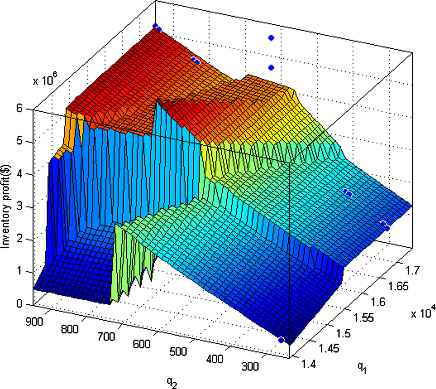
Inventory profit vs q₁ and q₂.

Table 2

Sensitivity analysis for the cloudy fuzzy model

Parameter	%Change	$q_{1}^{*}$	$q_{2}^{*}$	Z ^*
ρ	+30	16750	250	1366447
	+20	16864	364	1992454
	–20	17323	823	4496484
	–30	17438	938	5122491
σ	+30	17450	950	5192048
	+20	17332	832	4542855
	–20	16856	356	1946084
	–30	16737	237	1296891
r	+30	17094	594	3194550
	+20			3211190
	–20			3277749
	–30			3294389
c ₁	+30	17094	594	3166044
	+20			3192186
	–20			3296753
	–30			3322895
c ₃	+30	17094	594	3244319
	+20			3244369
	–20			3244569
	–30			3244619
p	+30	13934	260	501218
	+20	17094	594	1408076
	–20	17094	594	5080862
	–30	17094	594	5999059
s	+30	17094	594	7050975
	+20			5782140
	–20			706798
	–30			–

Figure 5 illustrate a comparative study of three cases in crisp and others fuzzy environment. From the figure, it is clear that case –(ii) gives the optimum value comparing with case –(i) and case –(iii). Among crisp and all fuzzy environments, cloudy fuzzy gives the optimum profit for all cases.

Figure 6 illustrate the sensitivity analysis of several parameters. From this figure, we see that cost parameters c₁, c₃ and discount rate r are almost insensitive parameters within this range (–30%to +30%) of variation. Moreover, the inventory profit gets remarkable variation when other parameters ρ, σ, p and s are changes from –30%to +30%. The basic managerial insight is that, inventory profit will not increase much more for increasing holding cost and set up cost up to 30%.

Figure 7 indicates the surface like curve of the inventory profit function with respect to the variation of the normal order quantity (q₁) and discount-based order quantity (q₂). It is seen that when the normal order quantity assumes values nearly 17094 units and the discounted order quantity assumes values about 900 units, the inventory profit becomes maximum. However, it is observed that when the normal order quantity assumes values nearly 13494 units and the discounted order quantity values nearly 900 units, the inventory profit becomes minimum. The inventory profit gets value within $(3100000–5000000) with respect to the normal order quantity range (16000–17000) units and that of discounted order quantity range (500–700) units. For the other cases, the profit function gets lesser values.

9 Advantages and disadvantages of the proposed model

9.1 Advantages

Sce the demand rate assumes cloudy fuzzy numbers, so it is more practical to analyse the model.

There is no need to incorporate screening cost as the customers themselves screen the items during their purchase.

This model is valid with the new defuzzification methods.

9.2 Disadvantages

The nature of the model may vary with the assumption of some other fuzzy parameters.

The result of the model may differ if the parameters assume different fuzzy numbers.

10 Conclusion

In this study, we have discussed an EOQ model of imperfect items that customers screened during the purchase. The low demand items are sold at discount rates among the customers. For a comparative study, we also consider demand rate as dense fuzzy number, cloudy fuzzy number, parabolic fuzzy number and degree of fuzziness. Throughout the study the numerical result and graphical illustration claim that the model gives finer optimum for cloudy fuzzy demand rate. So, cloudy fuzzy is much more suitable for decision-makers of an inventory problem to make decisions compared with others existing fuzzy environments. Thus, the basic novelties of this article are

Inventory problems should be optimized with the help of cloudy fuzzy rules instead of dense fuzzy, parabolic fuzzy and degree of fuzziness rule.

An Optimum solution can be obtained easily by a computer-based algorithm.

Increasing demand does not always imply the increase of inventory profit.

Scope of future work

The proposed fuzzy numbers can be used to solve other inventory model to get better solution.

Conflicts of interest

The authors declare that there is no conflict of interest regarding the publication of the article.

Footnotes

Acknowledgments

The authors are thankful to the honourable Editor-in chief, Associate Editors and anonymous reviewers for their valuable comments and suggestions to improve the quality of this article.

References

Sofiana

, Rosyidi

C.N.

, Integrated vendor-buyer inventory model considering imperfect quality and inspection errors with controllable lead time, Int. Conf. on Industrial Engineering and Engineering Management (IEEM), Singapore (2017), 1321–1325.

Faritha

A.A.

and Priya

, Optimizing triangular parabolic fuzzy EOQ model with shortage using nearest interval approximation, Int J Future Revolution Computer Sci Communication Eng 3 (2017), 92–96.

Baez-Sanchez

A.D.

, Moretti

A.C.

and Rojas-Medar

M.A.

, On polygonal fuzzy sets and numbers, Fuzzy Sets and System 209 (2012), 54–65.

Harris

F.W.

, Operations and costs (Factory Management Series), A. W. Shaw Co, Chicago (1913), 18–52.

Garg

, and Ansha, Arithmetic operations on generalized parabolic fuzzy numbers and its application, , Proc Natl Acad Sci India Sect A Phys Sci 88 (2018), 15–26.

Wangsa

I.D.

, Wee

H.M.

, A vendor-buyer inventory model for defective items with errors in inspection, stochastic lead time and freight cost, INFOR: Information Systems and Operational Research, 2019, https://doi.org/10.1080/03155986.2019.1607807.

Atanassov

K.T.

, Intuitionistic fuzzy sets, VII ITKR’s Session, Sofia, 1983.

Zadeh

L.A.

, Fuzzy sets, Information and Control 8(3) (1965), 338–356.

Khan

, Jaber

M.Y.

and Bonney

, An economic order quantity (EOQ) for items with imperfect quality and inspection errors, International Journal of Production Economics, 133(1) (2011), 118–113.

10.

Naimi

and Tahayori

, Centroid of polygonal fuzzy sets, Applied Soft Computing 95 (2020), https://doi.org/10.1016/j.asoc.2020.106519.

11.

Kazemi

, Olugu

E.U.

and Salwa

A-R.

, Hanim and R.A.B.R. Ghazilla, Development of a fuzzy economic order quantity model for imperfect quality items using the learning effect on fuzzy parameters, Journal of Intelligent and Fuzzy System 28(5) (2015), 2377–2389.

12.

Das

, De

S.K.

, Sana

S.S.

, An EOQ model for time dependent backlogging over idle time : A step order fuzzy approach, International Journal of Applied and Computational Mathematics, 2014, https://doi.org/10.1007/s40819-014-0001-y.

13.

Liang

, Wang

J.Q.

, A linguistic intuitionistic cloud decision support model with sentiment analysis for product selection in E-commerce, International Journal of fuzzy system. 2019, https://doi.org/10.1007/s40815-019-00606-0.

14.

Bellman

R.E.

and Zadeh

L.A.

, Decision making in a fuzzy environment, Management Sciences 17(4) (1970), 141–164.

15.

Karlin

, One stage inventory models with uncertainty, Studies in the Mathematical Theory of Inventory and Production, Stanford University Press, Stanford, CA. 1958.

16.

Karmakar

, De

S.K.

and Goswami

, A pollution sensitive dense fuzzy economic production quantity model with cycle time dependent production rate, Journal of Cleaner Production 154 (2017), 150–139.

17.

Karmakar

, De

S.K.

, Goswami

, A pollution sensitive remanufacturing model with waste items: Triangular dense fuzzy lock set approach, Journal of Cleaner Production, 2018, https://doi.org/10.1016/j.jclepro.2018.03.161.

18.

Maity

, Chakraborty

, De

S.K.

, Mondal

S.P.

, Alam

, A comprehensive study of a backlogging EOQ model with nonlinear heptagonal dense fuzzy environment, RAIRO-operations research. 2018, https://doi.org/10.1051/ro/201811.

19.

Maity

, De

S.K.

and Pal

, Two decision makers’ single decision over a back order EOQ model with dense fuzzy demand rate, Finance and Market 3 (2018), 1–11.

20.

Maity

, De

S.K.

, Mondal

S.P.

, A study of a backorder EOQ model for cloud-type intuitionistic dense fuzzy demand rate, Int. J. Fuzzy Syst, 2019, https://doi.org/10.1007/s40815-019-00756-1.

21.

Maity

, De

S.K.

, Mondal

S.P.

, A Study of an EOQ Model under Lock Fuzzy Environment, Mathematics, 2019, https://doi.org/10.3390/math7010075.

22.

S.K.

, Mahata

G.C.

, A cloudy fuzzy economic order quantity model for imperfect-quality items with allowable proportionate discounts, Journal of Industrial Engineering International, 2019, https://doi.org/10.1007/s40092-019-0310-1.

23.

S.K.

and Mahata

G.C.

, A Solution of an EOQ model for Imperfect Quality Items with Lock Fuzzy Controllable Demand and Discount, The Journal of Fuzzy Mathematics 28(2) (2020), 17–1.

24.

S.K.

, Mahata

G.C.

, Decision of a fuzzy inventory with fuzzy backorder model under cloudy fuzzy demand rate, International Journal of Applied and Computational Mathematics, (2016), https://doi.org/10.1007/s40819-016-0258-4.

25.

S.K.

and Beg

, Triangular dense fuzzy Neutrosophic sets, Neutrosophic Sets and Systems 13 (2016b), 1–12.

26.

S.K.

, Beg

, Triangular dense fuzzy sets and new defuzzication methods, Journal of Intelligent and Fuzzy System, 2016a, https://doi.org/10.3233/IFS-162160.

27.

S.K.

, Sana

S.S.

, The (p, q, r, l) model for stochastic demand under intuitionistic fuzzy aggregation with Bonferroni mean, Journal of Intelligent Manufacturing, 2016, https://doi.org/10.1007/s10845-016-1213-2.

28.

S.K.

, Goswami

and Sana

S.S.

, An interpolating by pass toPareto optimality in intuitionistic fuzzy technique for an EOQ modelwith time sensitive backlogging, Applied Mathematics and Computation 230 (2014), 664–674.

29.

S.K.

, EOQ model with natural idle time and wrongly measured demand rate, International Journal of Inventory Control and Management 3(1–2) (2013), 329–354.

30.

S.K.

, On Degree of Fuzziness and Fuzzy Decision Making, Cybernetics and System, 2020, https://doi.org/10.1080/01969722.2020.1723872.

31.

S.K.

, Triangular Dense Fuzzy Lock Set, Soft Computing, 2017, https://doi.org/10.1007/s00500-017-2726-0.

32.

Lin

T.Y.

and Chen

M.T.

, An economic order quantity model with screening errors, returned cost, and shortages under quantity discounts, African Journal of Business Management 5(4) (2011), 1129–1135.

33.

Zhou

, Chen

, Li

and Zhong

, A synergic economic order quantity model with trade credit, shortages, imperfect quality and inspection errors, Applied Mathematical Modelling 40(2) (2016), 1012–1028.