A heuristics pulse algorithm with relaxation pruning strategy for resources re-initialized UAV path planing

Abstract

Path planning is the basis and prerequisite for unmanned aerial vehicle (UAV) to perform tasks, and it is important to achieve precise location in path planning. This paper focuses on solving the UAV path planning problem under the constraint of system positioning error. Some nodes can re-initiate the accumulated flight error to zero and this type of scenario can be modeled as the resource-constrained shortest path problem with re-initialization (RCSPP-R). The additional re-initiation conditions expand the set of viable paths for the original constrained shortest path problem and increasing the search cost. To solve the problem, an effective preprocessing method is proposed to reduce the network nodes. At the same time, a relaxed pruning strategy is introduced into the traditional Pulse algorithm to reduce the search space and avoid more redundant calculations on unfavorable scalable nodes by the proposed heuristic search strategy. To evaluate the accuracy and effectiveness of the proposed algorithm, some numerical experiments were carried out. The results indicate that the three strategies can reduce the search space by 99%, 97% and 80%, respectively, and in the case of a large network, the heuristic algorithm combining the three strategies can improve the efficiency by an average of 80% compared to some classical solution.

Keywords

UAV path planing constraints shortest paths resource re-initialized pulse algorithm heuristics

1 Introduction

The path planning is becoming one of the key technologies of the unmanned aerial vehicle (UAV) autonomous control module [13] and the main purpose of drone path planning is to design a flight path directed to the target with the low-cost, i.e., the minimal probability of being destroyed with the UAV performance requirements [17]. Therefore, the path planning problem can be viewed as a complex optimization problem that requires efficient algorithms to solve [10].

The RCSPP is a classical problem in combinatorial optimization and there exists a part of the path planning problems can be modeled as the resource constrained shortest problem (RCSPP) where a quantity of resource in the network and the aim of RCSPP is to find a path with the smallest cost, such that resource consumption is less than the maximum amount of available resource [9]. The applications of RCSPP include robot global path planning [14, 18], intelligent transportation cloud computing system [4], UAV task path planning [10, 11] and so on.

When there are resource reset nodes in the network, the cumulative resources on the path are reinitialized to zero, and the problem is transformed into resource-constrained shortest path problem with re-initialization (RCSPP-R). Compared with RCSPP, there are relatively few literatures about RCSPP-R or its similarity. Cabral [2] considers the shortest path problem with relays (SPPR), which is similar to RCSPP-R, a path can accumulate no more than a given resource limit before replenishment must occur as while and uses the structure of feasible path, regards the optimal path as a series of sub paths between reset nodes, and decomposes SPPR into multiple sub SPP (shortest path problem). While the algorithm is found to be far less efficient due to the combination operation of sub paths. To solve similar problems, Laporte and Pascal [5] proposed a label correcting algorithm in the network where all costs and weights are non negative integers, which takes advantage of the characteristic that the number of labels required by any node does not exceed the number of resources plus one. Based on the assumption that the resource limit is relatively low, a matrix that can store tags to increase memory usage in order to achieve better time performance. In order to improve the time efficiency of the label correction method, Smith and Boland [12] proposed a standard preprocessing process and boundary calculation method to reduce the search space and improve the time efficiency of the algorithm without increasing the memory usage.

In this paper, there are two re-initiable resources (vertical and horizontal errors), reset nodes have associated constraints and only one resource can be re-initiated. Compared with the traditional RCSPP-R, the problem is more complicated because the reset of multiple resources expands the range of solution space and traditional solutions may get local optimal solutions. To effectively solve the constrained shortest path problem of multi resource reset, a heuristic based on the Pulse algorithm (PA) [6] and the branch bounds algorithm is proposed, which is called Pulse-R. The search space is initially reduced by first removing arcs or nodes whose cumulative resources do not satisfy the constraints through maximum resource capacity and re-initiation constraints. Second, considering the differences in the re-initiation constraints of the resources, the relevant nodes are pruned using an inverse search to calculate the boundary cost and the boundary optimal path after they are properly relaxed. In addition, to further improve the efficiency of the algorithm, a heuristic strategy is proposed to optimize the node expansion method. A large number of numerical experiments have been used to evaluate the stability and effectiveness of the proposed strategy, and the proposed algorithm has been compared with label correction method [12], ant colony algorithm [1] and the PA [6], indicating the effectiveness of the solution.

The main contributions of this paper can be summarized as follows:

•The existence of multi resource re-initialized RCSPP-R is studied. Compared with the traditional RCSPP-R, the problem is more complicated due to the mutual initialization of multi resources;

•In order to solve the problem of multi resource re-initialization RCSPP-R, a high performance algorithm based on pulse algorithm is proposed;

•A loop free pruning strategy is developed, and the special condition of the problem (re-initialization constraint) is included in the preprocessing to reduce the network size;

•A heuristic pruning strategy is proposed, which uses relaxed reverse search to pre order the subsequent extended nodes, so as to improve the search efficiency of the algorithm;

The remainder of this article is organized as follows. In Section 2, we describe a system model that is navigated by a drone in the presence of error correction, and in Section 3, we give specific design steps for an algorithm that can effectively solve such problems. In Section 4, some numerical experiments are presented to discuss the performance of the proposed algorithm. Section 5 discusses the results obtained and the paper concludes in Section 6.

2 System model and problem formulation

Path planning in a complex environment is an important problem of intelligent aircraft control. Due to the limitation of the system structure, the positioning system of UAV cannot locate itself accurately. Once the positioning error accumulates to a certain extent, the task may fail. Therefore, it is important and necessary for intelligent aircraft path planning to correct the positioning error during flight.

2.1 System model

As shown in Fig. 1, We consider a path planning system for UAV under the constraint of flight error, which consists of vertical error and horizontal error. Here gives some notation for mathematical describing of the problem. Starting node S, destination node E and N other error correction nodes denoted by s₁, s₂, ⋯ , s_N. After setting s₀ = S and s_N+1 = E, all nodes in the system can be represented by A ={ s₀, s₁, s₂, ⋯ , s_N, s_N+1 }. Without loss of generality, the nodes set can be denoted by the simplified index set Λ = {0, 1, 2, . . . , N + 1}.

Fig. 1

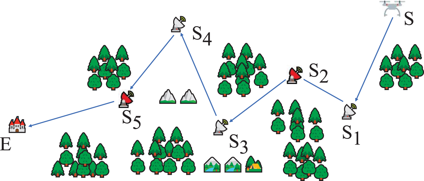
Scene of path planning based on UAV.

Regarding the evaluation of one candidate flight path, it can generally be constructed from fuel cost C_f and threat cost C_t as follows [7, 15]: $C = ξ C_{f} + (1 - ξ) C_{t}$ (1) where J is the weighted sum of cost for this path, and ξ represents the weighting parameter and when ξ is close to 1, a shorter path needs to be planned. As the threat cost is not considered at the moment in this paper, ξ is set to 1. Meanwhile for convenience presentation, the fuel cost is treated as the Euclidean distance between the nodes, i.e., the cost between node i and j is denoted as c_ij = d_ij =∥ s_i - s_j ∥.

Two types of nodes can correct only one of the horizontal error and vertical error independently. As shown in Figure 2, the horizontal error ɛ^h can be corrected by the black nodes and the vertical error ɛ^v can be corrected by the red nodes. ɛ^h will increase by δ_h after a flight over a unit distance and ɛ^h will increase by δ_v. For example, in the path fragment i → j, the cumulative horizontal error at node j (before correction) can be computed by plus a increment to the horizontal error at node i (after correction), i.e. 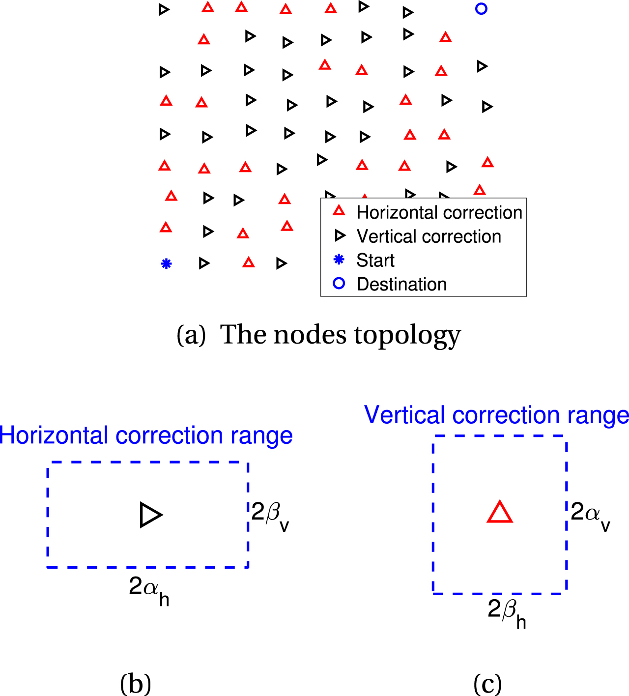${\hat{ɛ}}_{j}^{h} = ɛ_{i}^{h} + δ_{h} \cdot d_{ij}$ , similarly, ${\hat{ɛ}}_{j}^{v} = ɛ_{i}^{v} + δ_{v} \cdot d_{ij}$ . The horizontal (or vertical) error will be re-initialized to zero after a succeed correction. The correction ranges are shown in Figure 2. The initial error is 0 at the starting node S and the maximal allowable horizontal (vertical) should be no more than θ_h (θ_v).

Fig. 2

A two-dimensional case and the correction ranges.

After necessary error correction in some nodes, the UAV can arrive the destination with the error constraints satisfied. However, there are some difficult in searching a shortest path with such a re-initialization condition. First, the constraints formulation are related to the nodes type and nodes serial in a candidate path. They are changed with path evolution. Second, the additional re-initialization role expands the feasible path set and some traditional algorithms can’t achieve expected efficiency even lead to fail. We will give the solution in the following sections.

2.2 Problem formulation

The goal is to find a shortest path with the error constraints satisfied in the UAV system. After introducing some binary constants T_i, the related optimization problem, which is based on [3, 16], can be mathematically formulated as

$min \sum_{i, j \in Λ} x_{ij} \cdot c_{ij}$ (2) s.t. $\sum_{j \neq i} x_{ij} - \sum_{j \neq i} x_{ji} = △_{i}, \forall i \in Λ$ (3) $[\begin{matrix} T_{j} & 0 \\ 0 & 1 - T_{j} \end{matrix}] [\begin{matrix} ɛ_{i}^{h} + δ_{h} \cdot d_{ij} \\ ɛ_{i}^{v} + δ_{v} \cdot d_{ij} \end{matrix}] \leq [\begin{matrix} θ_{h} \\ θ_{v} \end{matrix}], \forall x_{ij} = 1$ (4) $[\begin{matrix} ɛ_{i}^{h} + δ_{h} \cdot d_{ij} \\ ɛ_{i}^{v} + δ_{v} \cdot d_{ij} \end{matrix}] \leq [\begin{matrix} α_{h} & β_{h} \\ β_{v} & α_{v} \end{matrix}] [\begin{matrix} 1 - T_{j} \\ T_{j} \end{matrix}], \forall x_{ij} = 1$ (5) $x_{ij} \in {0, 1}, \forall i, j \in Λ$ (6) $ɛ_{0}^{v} = 0, ɛ_{0}^{h} = 0$ (7) where the logic variables x_ij indicates whether to choose the arc(s_i, s_j) and △_i means a characteristic that $△_{i} = {\begin{matrix} 1, & s_{i} = S \\ - 1, & s_{i} = E \\ 0, & otherwise . \end{matrix}$ (8) The correction type of the node i is represented by T_i, and specifically, T_i = 0 means the node i can correct the horizontal error and T_i = 1 means a vertical error correction node.

The above optimization problem is very different from the traditional constrained path planning because the resource (i.e. flight error) in the problem can be re-initialized, and the constraints are linked to the accumulated resource consumption which is changed with the path evolution. In order to solve this problem effectively, we introduce a heuristic strategy and a relaxation pruning strategy to the Pulse algorithm [6].

3 Improved pulse algorithm

The Pulse algorithm [6] only propagates one pulse at each moment, and another pulse starts when it reaches the end or is cut by the pruning strategy. Fig. 3 shows the flow of the Pulse algorithm. In order to reduce the search space, three pruning strategies are used: (1) infeasible pruning is used to judge whether the current path is valid; (2) Bounds pruning narrows the search range of the algorithm through the current optimal cost; (3) Rollback pruning is used to reevaluate whether the previous node is selected correctly when the algorithm is extended to a certain point. While the boundary pruning strategy in the Pulse algorithm only aims at the monotonic increase or decrease of accumulated resources, so the traditional Pulse algorithm can not solve the optimization problem (2).

Fig. 3

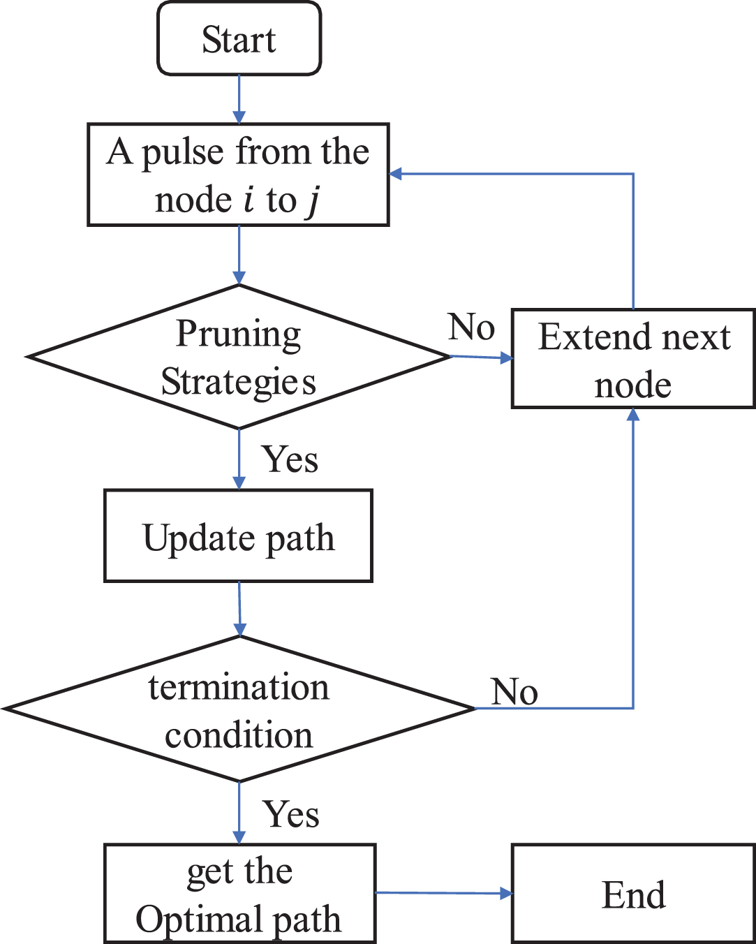
The flow chart of the Pulse algorithm.

3.1 The algorithm frame

To distinguish it from the original algorithm, it is named Pulse-R for the proposed algorithm. The algorithm consists of two phases: (1) in the delimitation stage, the lower limit of path length from each node to the destination node can be calculated by relaxation constraints; (2) in the recursive exploration stage, the pulse is transmitted recursively based on depth-first search until the pulse extends to the end or is cut off. In the recursive exploration phase, the pulse will store the current optimal solution of each node, avoiding the need to store all nodes’ information. To reduce the search space, different pruning strategies are used on each node to try to prevent pulse propagation. Algorithm 1 outlines the Pulse-R algorithm.

Algorithm 1 Pulse-R algorithm
Input:S, E, θ , {α_v, β_h, α_h, β_v},
Output:p^*, The optimal path; c (E), The optimal distance;
1: zeros( p ), zeros( D )
2: $ɛ_{i}^{h} \leftarrow 0, ɛ_{i}^{v} \leftarrow 0$
3: B =preprocessing(α_v, β_h, α_h, β_v)
4: [ $\underline{D}$ , $\underline{p}$ ]=Bounds(α_v, β_h, α_h, β_v)
5: pulse-R( $i, ɛ_{i}^{h}, ɛ_{i}^{v}, D, p, θ, α_{v}, β_{h}, α_{h}, β_{v}, B$ )
6: Return p^*,c (E) = D (E)

Lines 1 to 3 initialize the path p which stores the parent of each node in the path and the path can be obtained by backtracking the nodes of the path storage matrix p . The cumulative distance matrix denoted by D (i) = c (i) where c (i) represents the minimum cumulative cost from S to i. Row 4 is preprocessing, which constructs an adjacency matrix and reduces the size of the search space in combination with an upper error limit θ = [θ_v, θ_h] (see 3.2). The fifth line is a computational procedure for the boundary matrix, which calculates a relaxed lower bound for each node in ϒ(see 3.3). Finally, line 6 starts with the starting node S to recursively call Pulse-R(see algorithm 2).

The recursive calling procedure for Pulse-R is exhibited by the algorithm 2. IsFeasible and IsBounds, respectively, representing two pruning strategies (see 3.3). The re-initialize in row 4 represents a correction for the accumulated flight error. The Pathacceleration function is represented as a heuristic policy using the lower bound path obtained in the boundary policy for node expansion (see 3.5). Lines 13-14 make a deep recursive extension to the rest of the child node k calling algorithm 2 for node j, where $γ (k) = {k \in ϒ | B (i, k) \neq inf, k \notin \underline{p} (j)}$ , where B is the distance adjacency matrix (see 3.2), and the slack path from node j to the destination node E is denoted by $\underline{p} (j)$ .

Algorithm 2 Pulse-R procedure
Input:j, $ɛ_{i}^{h}, ɛ_{i}^{v}$ , D (i), θ , {α_v, β_h, α_h, β_v}, p , $\underline{p} (j)$ , B ,
Output: void.
1: i is the parent node of j
2: if IsFeasible(j, $ɛ_{i}^{h}, ɛ_{i}^{v}, θ, α_{v}, β_{h}, α_{h}, β_{v}, B$ )=true
3: if IsBounds(j, D (i), $\underline{D} (i)$ )=true
4: $ɛ_{j}^{h}$ =re-initialize $(ɛ_{i}^{h}, j)$ or $ɛ_{j}^{v}$ =re-initialize $(ɛ_{i}^{v}, j)$
5: p (j) = i, D (j) = D (i) + B (i, j)
6: if Pathacceleration(j, p , $ɛ_{j}^{h}$ , $ɛ_{j}^{v}$ , D (j), $\underline{p} (j)$ )==true
7: b is the child node in $\underline{p} (j)$ of node j
8: re-initialize $ɛ_{b}^{h}$ or $ɛ_{m}^{v}$
9: p (b) = j, D (b) = D (j) + B (j, b)
10: Pulse-R( $m, ɛ_{m}^{h}, ɛ_{m}^{v}, D, p, θ, α_{v}, β_{h}, α_{h}, β_{v}, B$ )
11: else
12: fork ∈ Γ (j) do
13: Pulse-R( $k, ɛ_{j}^{h}, ɛ_{j}^{v}, D, p, θ, α_{v}, β_{h}, α_{h}, β_{v}, B$ )
14: end for
15: end if
16: end if
17: end if

3.2 Preprocessing

The process will construct a distance adjacency matrix B by combination with an upper limit of cumulative error θ , nodes that surpass the resource cumulative capacity limitation or violate the resource re-initiation constraint are eliminated during the construction of the correlation matrix. The maximum distance (which is based on (4)) denoted by L_v, L_h between node i and the expandable child node can be calculated as $L_{v} (i, j) = θ_{v} / δ_{v}; L_{h} (i, j) = θ_{h} / δ_{h} .$ (9)

From constrains (5), Specifically, the distance between node i, j must satisfy one of the following inequalities $\begin{matrix} d_{ij} \leq {\tilde{L}}_{v} (i, j); d_{ij} \leq {\tilde{L}}_{h} (i, j) \end{matrix}$ (10) where ${\tilde{L}}_{v} (i, j) = min {α_{v}, β_{h}} / δ_{v}$ , ${\tilde{L}}_{h} (i, j) = min {α_{h}, β_{v}} / δ_{h}$ then B (i, j) = d_ij, otherwise B (i, j) = inf.

Moreover, there will be a cycle in the viable path since flight error can be re-initiated. Obviously, this is not the optimal solution. To avoid the cycle, a no fallback strategy is proposed, which constructs an adjacency matrix by comparing the direct distance between the node and the starting node S. For example, as Fig. 4, an adjacency matrix of node i was constructed that satisfies the equations (9) and (10) and satisfies the assumption that the child nodes are jand k. The distance from the node i to S is expressed as ξ (i), and correspondingly, for the nodes j and k, the distance to S is ξ (j), ξ (k). If ξ (i) > ξ (j), it means that i to j are regressive relationships (in Fig. 4). To avoid cycle, set B (i, j) = inf, and conversely, if ξ (i) > ξ (k), then B (i, k) = d_ik.

Fig. 4

Two typical non optimal path segments.

Fig. 5

Original and relaxed correction constraint.

3.3 Pruning strategies

IsFeasible pruning. Discarding infeasible local paths is a commonly used method in labeling algorithm [8]. When a partial path reaches the node i and prepares to expand the node j, the strategy will check whether the node not worthy to be expanded and whether the capacity limit for resource accumulation is exceeded. If any of these events happen, the part is not feasible because it can be safely pruned. Moreover based on the branch and bound principle, pruning the feasible solution that does not satisfy the current optimal solution can reduce the search space of the solution. This pruning looks for the node which worthy of being expanded, and it checks the cost c′ (j) which between j and the starting node S is less than the current optimal cost c (j). If c′ (j) < c (j), the node j is reserved.

IsBounds Pruning. To restrict the search space more strictly, a boundary policy verifies whether the current node is worth expanding. Specifically, the partial path distance at the node j is c (j), and the boundary distance (the minimum path distance from node j to E)denoted by $\underline{c} (j)$ . If $c (j) + \underline{c} (j) > c (E)$ , it means that regardless of expanding the node after j the path does not yield a path smaller than the current minimum distance, and thus the node j can be safely pruned.

3.4 Bounds pruning

A bounder strategy that is based on lower bounds on the cost, is proposed. This boundary strategy stores the lower cost of the path length of each node, which is realized by relaxing the constraint condition of each correct node. That means that the cumulative error satisfies one of the following inequalities at node j (assuming that the horizontal error can be corrected, the same is true in other cases), $\begin{matrix} ɛ_{i}^{h} + δ_{h} \cdot d_{ij} > α_{h}, ɛ_{i}^{v} + δ_{v} \cdot d_{ij} > β_{v}, \end{matrix}$ (11) and the error correction cannot be performed at node j. If it can get a lower distance by expanding node i, the relevant constraints can be appropriately scaled and the lower bound of the distance $\underline{c} (i)$ can be calculated, obviously $\underline{c} (i) \leq c (i)$ . Therefore, the constraints of re-initialization nodes can be changed to the maximum value of resource constraints. The associated binding variation can be represented by Fig. 5 and the red dotted line is the relaxed correction constraint. Its calculation can be expressed as ${\begin{matrix} {\tilde{α}}_{v} = max {α_{v}, β_{h}}, {\tilde{β}}_{h} = max {α_{v}, β_{h}} \\ {\tilde{α}}_{h} = max {α_{h}, β_{v}}, {\tilde{β}}_{v} = max {α_{h}, β_{v}} . \end{matrix}$ (12)

Algorithm 3 Bounds
Input: ${\tilde{α}}_{v}, {\tilde{α}}_{h}, {\tilde{β}}_{v}, {\tilde{β}}_{h}$ , θ , B , T,
Output: $\underline{D}$ , lower bound matrix; $\underline{p}$ , lower bound path.
1: Initialize Queue Q, head=1,tail=1
2: zeros( $\underline{p}$ ), $ɛ_{T}^{h} = 0, ɛ_{T}^{v} = 0$ , $\underline{D} (T) = 0$
3: EnQueue (Q,T),head=head+1
4: while !QueueEmpty(Q) do
5: u=Q(tail)
6: fory ∈ Γ (u) do
7: if Is-Feasible( $u, y, ɛ_{u}^{h}, ɛ_{u}^{v}, θ, {\tilde{α}}_{v}, {\tilde{α}}_{h}, {\tilde{β}}_{v}, {\tilde{β}}_{h}$ )=true then
8: $\underline{p} (y) = u$ , $\underline{D} (y) = \underline{D} (u) + B (u, y)$
9: re-initialize $ɛ_{y}^{h}$ or $ɛ_{y}^{v}$
10: EnQueue (Q,y), head=head+1
11: end if
12: tail=tail+1
13: end for
14: end while

3.5 Path acceleration strategy

In the boundary pruning strategy proposed by Lozano et al. [6], only the lower bound of the path cost $\underline{c}$ is retained, and other information is not used, such as the path information corresponding to the lower bound of the path length of each node $\underline{p}$ . To improve the algorithm effectiveness, the heuristic strategy, which called path acceleration pruning strategy, is proposed.

Since the lower bound path $\underline{p}$ is calculated with the boundary strategy, some nodes in $\underline{p}$ cannot satisfy the resource constraints of the original problem. If the nodes that meet the resource constraints of the original problem can be found, the algorithm can directly expand these nodes without judging other nodes, which greatly improves the time efficiency of the algorithm.

For example, in Fig. 6, the dashes line as the shortest path. The node expansion way of traditional algorithms is shown in Fig. 6(a), expanding the children of each node in turn. The darker nodes in the graph represent the node extension of traditional algorithm, and it can be observed that almost all the nodes in the network are visited. The node extension range the proposed algorithm based on the heuristic strategy are represented by Fig. 6(b), where the dash-dotted line is the lower bound path corresponding to the starting node S. The algorithm scales along this path, expanding its children in the traditional way of node expansion if there is a node that does not satisfy the constraints (4), (5). The optimal path can be obtained quickly without extensive access to the nodes in the network.

Fig. 6

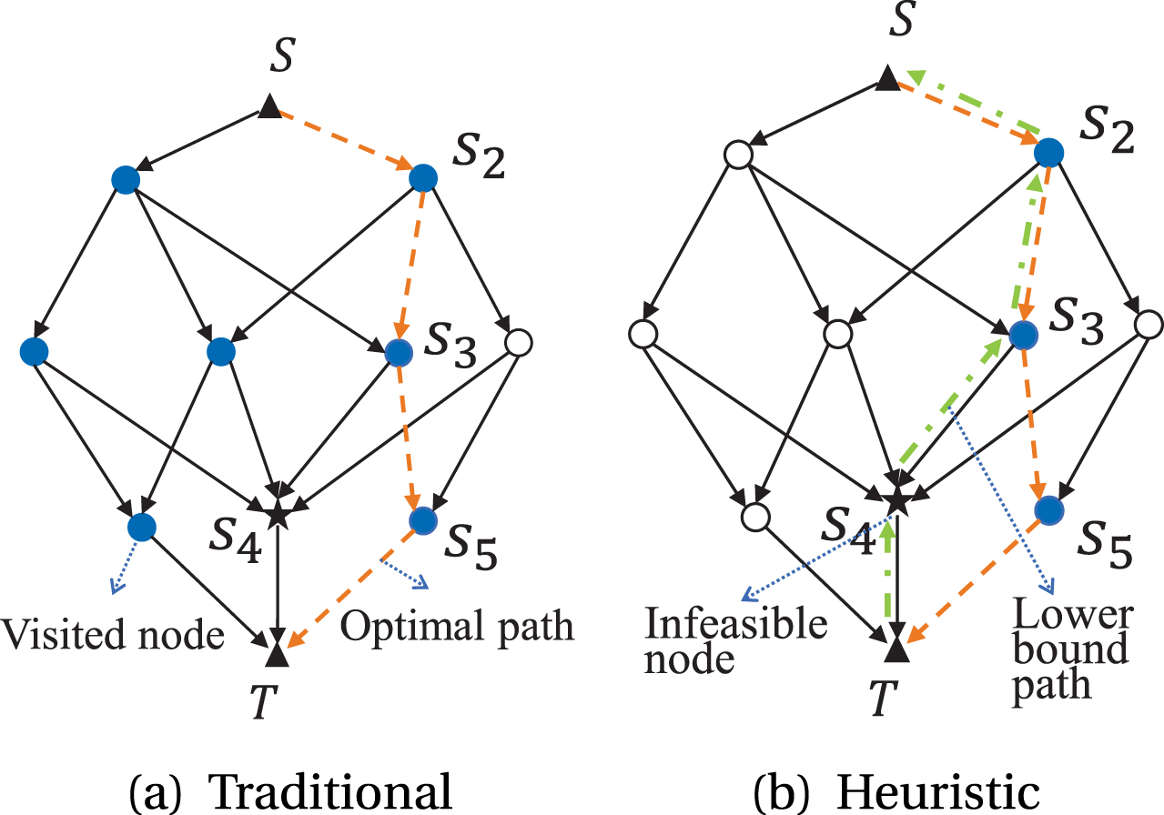
Node extension for traditional and heuristics.

4 Computational results

In this section, the proposed solution strategy will be evaluate and all algorithms have been coded in Matlab and the numerical results are carried out on an Intel(R) Core(TM) i5-1135G7 2.40 GHz 16.00GB RAM machine under Microsoft Windows 10. All computational times are reported in seconds.

4.1 Algorithms

The following seven algorithms will be used in comparative experiments.

LC denotes the label-correcting algorithm proposed in [12]. PA denotes the Pulse algorithm proposed in [6]. AC denotes the ant colony algorithm proposed in [1]. PRW solves the problem with Pulse-R does not use preprocessing and any pruning strategies in section 3. PRP solves the problem with Pulse-R uses preprocessing in section 3.2 but without uses any pruning strategies in section 3. PRB implements the preprocessing and bounds pruning in sections 3.2,3. PR denotes the complete Pulse-R algorithm which combines preprocessing, boundary strategy and heuristic search in section 3.5.

In order to make a fair comparison between the solution strategies under consideration, we use the same data structure to implement and modify them appropriately to solve the problem.

4.2 Instances

In order to construct the data set more objectively, the instances generation method similar to [12] is used to carry out the numerical experiments. The instances set used in the experiment is randomly generated and the three-dimensional coordinates of each node, and the range of x-axis, y-axis and z-axis are [0,100000]. Based on the experimental design in Smith[12], The resource re-initialized constraint is generated by 13 and the constraints used for the experiments can be viewed by Table 1. To verify the influence of different types of re-initialized node distributions on the proposed algorithm, the network is constructed by using re-initialized nodes based on different distributions, and each network is randomly generated by section 4.1. In the network with the same number of nodes corresponding to different constraints, only the correction type of nodes is changed. The nodes are respectively uniformly distributed (1, N), normal distribution (N/2, N/4) and the exponential distribution (N/2), where N is the number of network nodes.

Table 1
The constrain of network

Constrain Type Variable value

Constrain I γ₁ = 0, γ₂ = 1, η₁ = 1, η₂ = 0, λ = 0

Constrain II γ₁ = 0.2, γ₂ = 0.8, η₁ = 0.7, η₂ = 0.3, λ = 0.3

Constrain III γ₁ = 1/3, γ₂ = 0.6, η₁ = 2/3, η₂ = 0.4, λ = 0.5

Constrain IV γ₁ = 0.6, γ₂ = 0.5, η₁ = 0.4, η₂ = 0.6, λ = 0.7

Constrain V γ₁ = 0.8, γ₂ = 0.2, η₁ = 1/3, η₂ = 0.8, λ = 0.9

Constrain Type	Variable value
Constrain I	γ₁ = 0, γ₂ = 1, η₁ = 1, η₂ = 0, λ = 0
Constrain II	γ₁ = 0.2, γ₂ = 0.8, η₁ = 0.7, η₂ = 0.3, λ = 0.3
Constrain III	γ₁ = 1/3, γ₂ = 0.6, η₁ = 2/3, η₂ = 0.4, λ = 0.5
Constrain IV	γ₁ = 0.6, γ₂ = 0.5, η₁ = 0.4, η₂ = 0.6, λ = 0.7
Constrain V	γ₁ = 0.8, γ₂ = 0.2, η₁ = 1/3, η₂ = 0.8, λ = 0.9

${\begin{matrix} α_{v} = ⊔ (γ_{1} * α^{-} + (1 - γ_{1}) * α^{+}) \\ β_{h} = ⊔ (γ_{2} * ς^{-} + (1 - γ_{2}) * α_{v}) \\ β_{v} = ⊔ (η_{1} * β_{h} + (1 - η_{1}) * β^{+}), \\ α_{h} = ⊔ (η_{2} * β_{v} + (1 - η_{2}) * ς^{+}) \\ θ^{-} = max {α_{v}, β_{h}, α_{h}, β_{v}}, \\ θ_{v} = ⊔ (λ * θ^{-} + (1 - λ) * θ^{+}) \\ θ_{h} = ⊔ (λ * θ^{-} + (1 - λ) * θ^{+}) \end{matrix}$ (13) where γ₁,γ₂, η₁, η₂,λ are parameter which is a random number between 0 and 1 [12]. To ensure test different resource constraint, for each instance, using a lower resource limit denoted by α^-,ς^- and an upper resource limit denoted by α⁺,β⁺,ς⁺and θ⁺ are the upper limit. The ⊔ (·) is a floor function [12], i.e., the ⊔ (a) is the maximum integer no larger than a.

The coordinate of the starting node is (0,50000,5000) and the destination node is (100000,60000,5000). At the same time, setting the upper limit of the algorithm’s time consumption to 300 seconds, if the time consumed by the algorithm exceeds this upper limit, it is considered that the algorithm has no solution. The cost of each arc is the Euclidean distance and the α^- = 15, α⁺ = 25, β⁺ = 20, ς^- = 10, ς⁺ = 25, θ⁺ = 30 and the correlation coefficient δ_v = 0.001, δ_h = 0.001.

4.3 Performance of the pruning strategies

In order to comprehensively test the effectiveness of the proposed strategies. This section will test the performance of PRW, PRP, PRB and PR. The instances are randomly generated from Section 4.1.

Table 2 shows the average execution time(CPUs) of each algorithm in different networks, where the preprocessing time in PRW is to calculate the cost between any two nodes, without boundary computation time. Pretreatment times from Section 3.2 are used as included in the PRP, and boundary calculation times from Section 3 are also included in the PRB. PR contains the time for the preprocessing, boundary calculation, and heuristic strategies involved in this paper.

Table 2
Average time for Algorithm 1 with various pruning strategies

Constraint and grid Uniform Distribution Normal Distribution Exponential Distribution

Constraint Grid(N) PRW PRP PRB PR PRW PRP PRB PR PRW PRP PRB PR

I 400 15.1544 0.1024 0.0344 0.0280 12.9283 0.0833 0.0304 0.0271 13.4356 0.0658 0.0327 0.0292

I 600 45.2344 0.3007 0.0823 0.0600 42.8156 0.2697 0.0807 0.0680 43.4033 0.2807 0.0955 0.0842

I 800 97.2428 0.6085 0.1345 0.1032 94.4731 0.5683 0.1594 0.1461 96.2933 0.6055 0.1939 0.1712

I 1000 208.9372 1.2211 0.2126 0.1673 190.0902 1.4877 0.3113 0.2552 201.1444 1.2846 0.3130 0.2714

II 400 15.2187 0.0913 0.0345 0.0276 15.7136 0.1148 0.0541 0.0455 16.8524 0.1097 0.0545 0.0472

II 600 50.4817 0.2814 0.0794 0.0663 49.0062 0.3387 0.1083 0.0962 47.3860 0.2961 0.1132 0.1022

II 800 113.6245 0.5705 0.1263 0.1043 107.6319 0.6957 0.1924 0.1674 111.2972 0.7595 0.2127 0.1804

II 1000 204.4647 1.3693 0.2227 0.1754 208.7486 1.4504 0.2963 0.2574 210.2116 1.3902 0.3133 0.2749

III 400 12.5297 0.0868 0.0371 0.0301 13.9187 0.1054 0.0524 0.0443 12.3012 0.0952 0.0481 0.0445

III 600 40.2237 0.2479 0.0908 0.0751 38.5346 0.2489 0.1033 0.0936 39.9767 0.2800 0.1152 0.0996

III 800 94.8623 0.6242 0.1559 0.1341 89.5705 0.6790 0.1981 0.1711 92.1204 0.7199 0.2344 0.2104

III 1000 171.5830 1.1464 0.2491 0.2128 172.0081 1.1942 0.3751 0.3441 168.5949 1.3937 0.4058 0.3631

IV 400 10.1394 0.0698 0.0376 0.0344 9.7966 0.0761 0.0563 0.0536 9.7447 0.0891 0.0637 0.0587

IV 600 50.2176 0.2846 0.0988 0.0878 33.7402 0.2493 0.1312 0.1199 38.6365 0.2481 0.1396 0.1276

IV 800 121.8404 0.6649 0.1588 0.1421 121.9036 0.8862 0.2313 0.2063 130.2219 0.8027 0.2513 0.2238

IV 1000 186.0825 1.3014 0.2448 0.2078 190.0615 1.2672 0.3217 0.2999 186.9900 1.2314 0.3453 0.3214

V 400 6.3366 0.0495 0.0319 0.0296 6.8481 0.0697 0.0520 0.0480 7.5350 0.0583 0.0457 0.0437

V 600 53.2594 0.2500 0.0908 0.0752 30.1974 0.2328 0.1084 0.0996 54.4018 0.2712 0.1059 0.0892

V 800 88.6776 0.5421 0.1614 0.1348 107.1404 0.7172 0.2069 0.1640 93.7815 0.5978 0.2288 0.2104

V 1000 144.1775 0.9871 0.2326 0.2086 138.5005 1.0436 0.3590 0.3321 152.5514 1.0426 0.3417 0.3209

Constraint and grid	Uniform Distribution	Normal Distribution	Exponential Distribution
I	400	15.1544	0.1024	0.0344	0.0280	12.9283	0.0833	0.0304	0.0271	13.4356	0.0658	0.0327	0.0292
I	600	45.2344	0.3007	0.0823	0.0600	42.8156	0.2697	0.0807	0.0680	43.4033	0.2807	0.0955	0.0842
I	800	97.2428	0.6085	0.1345	0.1032	94.4731	0.5683	0.1594	0.1461	96.2933	0.6055	0.1939	0.1712
I	1000	208.9372	1.2211	0.2126	0.1673	190.0902	1.4877	0.3113	0.2552	201.1444	1.2846	0.3130	0.2714
II	400	15.2187	0.0913	0.0345	0.0276	15.7136	0.1148	0.0541	0.0455	16.8524	0.1097	0.0545	0.0472
II	600	50.4817	0.2814	0.0794	0.0663	49.0062	0.3387	0.1083	0.0962	47.3860	0.2961	0.1132	0.1022
II	800	113.6245	0.5705	0.1263	0.1043	107.6319	0.6957	0.1924	0.1674	111.2972	0.7595	0.2127	0.1804
II	1000	204.4647	1.3693	0.2227	0.1754	208.7486	1.4504	0.2963	0.2574	210.2116	1.3902	0.3133	0.2749
III	400	12.5297	0.0868	0.0371	0.0301	13.9187	0.1054	0.0524	0.0443	12.3012	0.0952	0.0481	0.0445
III	600	40.2237	0.2479	0.0908	0.0751	38.5346	0.2489	0.1033	0.0936	39.9767	0.2800	0.1152	0.0996
III	800	94.8623	0.6242	0.1559	0.1341	89.5705	0.6790	0.1981	0.1711	92.1204	0.7199	0.2344	0.2104
III	1000	171.5830	1.1464	0.2491	0.2128	172.0081	1.1942	0.3751	0.3441	168.5949	1.3937	0.4058	0.3631
IV	400	10.1394	0.0698	0.0376	0.0344	9.7966	0.0761	0.0563	0.0536	9.7447	0.0891	0.0637	0.0587
IV	600	50.2176	0.2846	0.0988	0.0878	33.7402	0.2493	0.1312	0.1199	38.6365	0.2481	0.1396	0.1276
IV	800	121.8404	0.6649	0.1588	0.1421	121.9036	0.8862	0.2313	0.2063	130.2219	0.8027	0.2513	0.2238
IV	1000	186.0825	1.3014	0.2448	0.2078	190.0615	1.2672	0.3217	0.2999	186.9900	1.2314	0.3453	0.3214
V	400	6.3366	0.0495	0.0319	0.0296	6.8481	0.0697	0.0520	0.0480	7.5350	0.0583	0.0457	0.0437
V	600	53.2594	0.2500	0.0908	0.0752	30.1974	0.2328	0.1084	0.0996	54.4018	0.2712	0.1059	0.0892
V	800	88.6776	0.5421	0.1614	0.1348	107.1404	0.7172	0.2069	0.1640	93.7815	0.5978	0.2288	0.2104
V	1000	144.1775	0.9871	0.2326	0.2086	138.5005	1.0436	0.3590	0.3321	152.5514	1.0426	0.3417	0.3209

On average, the preprocessing process is very useful in improving the efficiency of the algorithm. In fact, we can conclude that almost all PRB calculations in Table 2 take more than 10 seconds, while PRP is only 1.5 seconds at most. With the increase of the number of network nodes, the calculation time of PRB almost presents an exponential growth trend. In addition, the average computing time of PRB is less than 0.15 seconds, which indicates that the addition of boundary strategy can further reduce the time consumption of the algorithm. At the same time, the time consumption of PR integrating all strategies is lower, even to the constraint V, when the number of network nodes is 1000, it only consumes 0.2 seconds, which is 1500 times higher than the PRW efficiency. On the other hand, the performance of PR algorithm under three different distributions is almost the same.

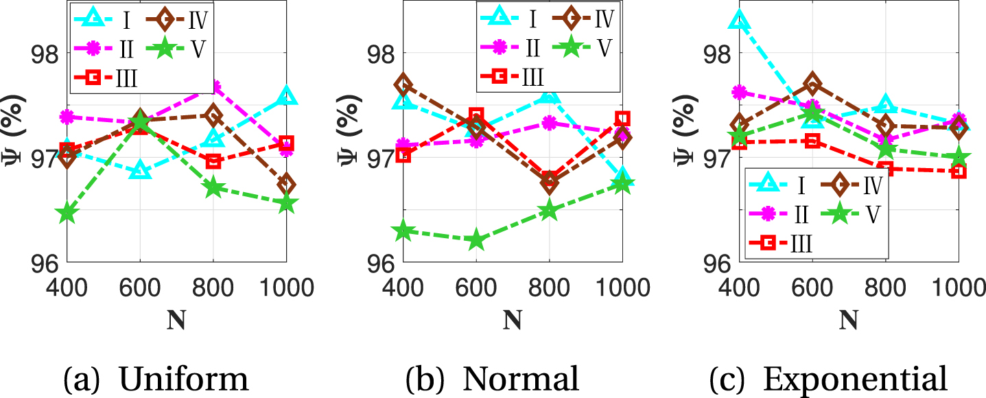
To better highlight the benefits of each strategy in the article, Figures 7, 8 and 9 respectively show the percentage of node extensions of the algorithm using preprocessing, boundary policy and heuristic search strategy ψ, that is $Ψ = (n_{m} - n_{PR}) / n_{m} * 100 % .$ (14) where the n_PR is the number of node expansions of PR, and n_m is the number of other algorithms. From these graphs, we can get that the use of preprocessing greatly reduces redundant nodes, which makes the node expansion times of the algorithm reduced by 97.6%, and the boundary strategy can be reduced by 96.2% as much as using preprocessing process, while heuristic search strategy can reduce 96% on the basis of boundary strategy. In addition, it can be concluded that the more nodes are, the better the pruning effect is, which explains the reason for the rapid decrease of time consumption in Table 2.

Fig. 7

Node extensions comparison (PRW vs PRP).

Fig. 8

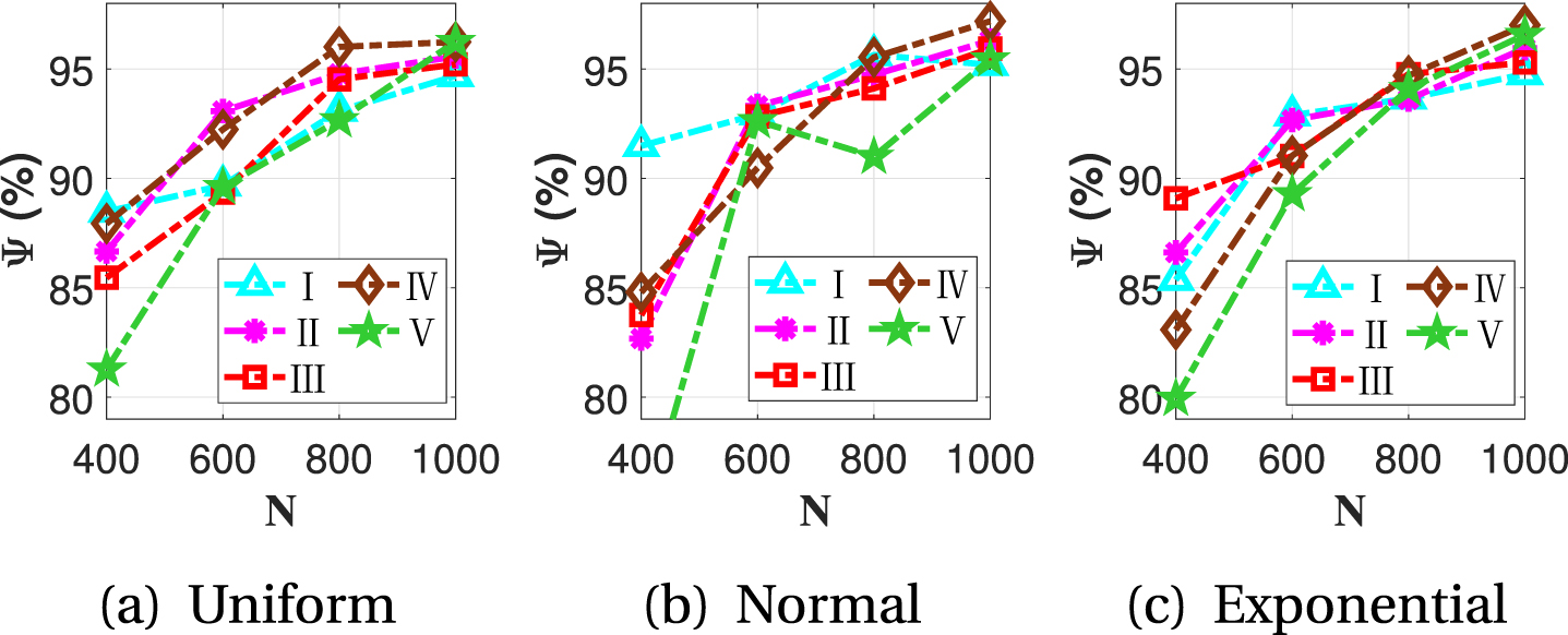
Node extensions comparison (PRP vs PRB).

Fig. 9

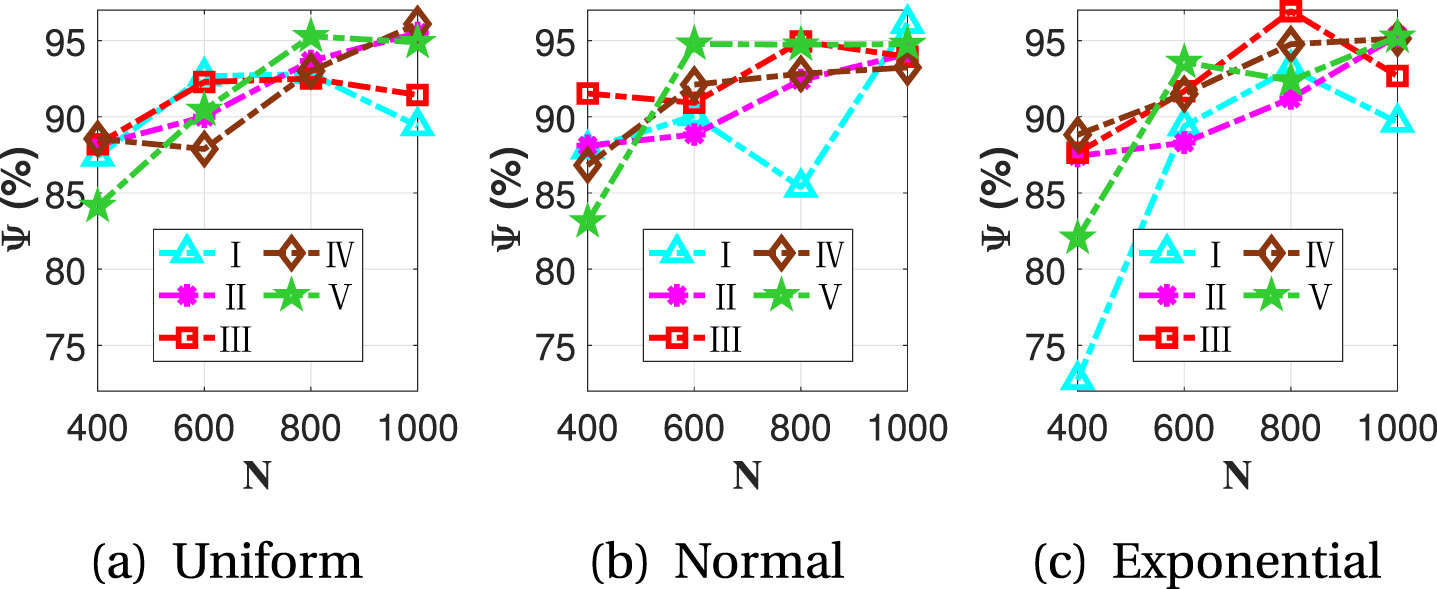
Node extensions comparison (PRB vs PR).

Furthermore, to evaluate the effectiveness of PR algorithm under different cost indicators, six test sets were randomly generated in a fixed network with constraint II, number of network nodes 800 in which the cost weight in each test set obeyed (0.3, 0.05) normal distribution.The convergence curve of the PR algorithm is shown in Fig. 10. it can conclude that the PR algorithm has a better convergence rate, and all of the PR algorithms in six instances can converge near the fixed cost and indicating the effectiveness of the proposed algorithm.

Fig. 10

Comparative convergence curves of algorithms.

4.4 Compared with other algorithms

To test the effectiveness and accuracy of the proposed algorithm, the performance of LC, PA, AC and PR will be calculated in this section, and the instances are randomly generated from Section 4.1.

Table 3 shows the average execution time (CPUs) of LC, PA, PR and AC in different networks, including preprocessing and boundary calculation time. It can be concluded from the table that in addition to AC, the other three algorithms consume less time, which indicates that the scale of network nodes is within a certain range, and the swarm intelligence algorithm has time efficiency compared to the deterministic algorithm. In addition, PR and PA are based on the depth-first search idea. When the number of nodes is small (such as 600 or less), the time consumption of LC will be better than the two, but as the number of nodes increases, the effect of the boundary strategy begins to gradually Increase, so that the time consumption of PR and PA when the number of nodes is more than 800 is less than that of LC. On the other hand, the tests of different strategies in Section 3.5 show that it is effective in improving the efficiency of the algorithm, so the calculation time of PR is smaller than that of PA.

Table 3
Average time for various algorithms in different constraint

Constraint and grid Uniform Distribution Normal Distribution Exponential Distribution

Constraint Grid(N) LC PA PR AC LC PA PR AC LC PA PR AC

I 400 0.0279 0.0592 0.0280 2.1894 0.0275 0.0459 0.0271 2.2362 0.0290 0.0504 0.0292 2.2740

I 600 0.0603 0.1570 0.0600 3.4021 0.0705 0.1239 0.0680 3.1032 0.0861 0.1379 0.0842 3.0821

I 800 0.1086 0.2273 0.1032 4.4984 0.1497 0.2094 0.1461 4.3780 0.1782 0.2738 0.1712 4.2986

I 1000 0.1755 0.3316 0.1673 6.6447 0.2683 0.4476 0.2552 6.4650 0.2790 0.4429 0.2714 6.0291

II 400 0.0270 0.0574 0.0276 2.8649 0.0444 0.0897 0.0455 3.1617 0.0468 0.0773 0.0472 3.2073

II 600 0.0691 0.1212 0.0663 4.2819 0.0978 0.1505 0.0962 4.2185 0.1044 0.1517 0.1022 4.2801

II 800 0.1130 0.1837 0.1043 5.7901 0.1756 0.2580 0.1674 5.8226 0.1861 0.2996 0.1804 5.7682

II 1000 0.1899 0.3341 0.1754 7.7342 0.2735 0.3939 0.2574 7.7795 0.2909 0.4123 0.2749 7.5639

III 400 0.0299 0.0596 0.0301 2.7664 0.0438 0.0796 0.0443 3.0541 0.0446 0.0650 0.0445 2.7161

III 600 0.0769 0.1441 0.0751 3.8480 0.0967 0.1379 0.0936 3.7147 0.1015 0.1611 0.0996 3.8593

III 800 0.1401 0.2240 0.1341 5.1184 0.1794 0.2759 0.1711 5.0884 0.2188 0.3056 0.2104 5.1944

III 1000 0.2234 0.3525 0.2128 6.7632 0.3591 0.4570 0.3441 6.5359 0.3769 0.5183 0.3631 6.6466

IV 400 0.0339 0.0505 0.0344 5.2433 0.0533 0.0686 0.0536 4.1638 0.0590 0.0788 0.0587 3.5878

IV 600 0.0901 0.1362 0.0878 7.2955 0.1221 0.1661 0.1199 4.3541 0.1300 0.1695 0.1276 4.9565

IV 800 0.1530 0.2030 0.1421 8.6752 0.2170 0.2953 0.2063 9.3951 0.2354 0.3143 0.2238 9.5005

IV 1000 0.2255 0.3288 0.2078 9.2852 0.3152 0.3777 0.2999 9.4290 0.3381 0.4010 0.3214 9.0835

V 400 0.0286 0.0431 0.0296 13.9465 0.0461 0.0698 0.0480 10.5765 0.0426 0.0564 0.0437 26.5724

V 600 0.0770 0.1407 0.0752 16.5208 0.1017 0.1360 0.0996 7.4518 0.0920 0.1545 0.0892 13.4483

V 800 0.1427 0.2275 0.1348 10.7713 0.1721 0.3177 0.1640 15.0567 0.2161 0.2854 0.2104 10.0034

V 1000 0.2219 0.2990 0.2086 10.2709 0.3439 0.4369 0.3321 11.1575 0.3348 0.3988 0.3209 9.6829

Constraint and grid	Uniform Distribution	Normal Distribution	Exponential Distribution
I	400	0.0279	0.0592	0.0280	2.1894	0.0275	0.0459	0.0271	2.2362	0.0290	0.0504	0.0292	2.2740
I	600	0.0603	0.1570	0.0600	3.4021	0.0705	0.1239	0.0680	3.1032	0.0861	0.1379	0.0842	3.0821
I	800	0.1086	0.2273	0.1032	4.4984	0.1497	0.2094	0.1461	4.3780	0.1782	0.2738	0.1712	4.2986
I	1000	0.1755	0.3316	0.1673	6.6447	0.2683	0.4476	0.2552	6.4650	0.2790	0.4429	0.2714	6.0291
II	400	0.0270	0.0574	0.0276	2.8649	0.0444	0.0897	0.0455	3.1617	0.0468	0.0773	0.0472	3.2073
II	600	0.0691	0.1212	0.0663	4.2819	0.0978	0.1505	0.0962	4.2185	0.1044	0.1517	0.1022	4.2801
II	800	0.1130	0.1837	0.1043	5.7901	0.1756	0.2580	0.1674	5.8226	0.1861	0.2996	0.1804	5.7682
II	1000	0.1899	0.3341	0.1754	7.7342	0.2735	0.3939	0.2574	7.7795	0.2909	0.4123	0.2749	7.5639
III	400	0.0299	0.0596	0.0301	2.7664	0.0438	0.0796	0.0443	3.0541	0.0446	0.0650	0.0445	2.7161
III	600	0.0769	0.1441	0.0751	3.8480	0.0967	0.1379	0.0936	3.7147	0.1015	0.1611	0.0996	3.8593
III	800	0.1401	0.2240	0.1341	5.1184	0.1794	0.2759	0.1711	5.0884	0.2188	0.3056	0.2104	5.1944
III	1000	0.2234	0.3525	0.2128	6.7632	0.3591	0.4570	0.3441	6.5359	0.3769	0.5183	0.3631	6.6466
IV	400	0.0339	0.0505	0.0344	5.2433	0.0533	0.0686	0.0536	4.1638	0.0590	0.0788	0.0587	3.5878
IV	600	0.0901	0.1362	0.0878	7.2955	0.1221	0.1661	0.1199	4.3541	0.1300	0.1695	0.1276	4.9565
IV	800	0.1530	0.2030	0.1421	8.6752	0.2170	0.2953	0.2063	9.3951	0.2354	0.3143	0.2238	9.5005
IV	1000	0.2255	0.3288	0.2078	9.2852	0.3152	0.3777	0.2999	9.4290	0.3381	0.4010	0.3214	9.0835
V	400	0.0286	0.0431	0.0296	13.9465	0.0461	0.0698	0.0480	10.5765	0.0426	0.0564	0.0437	26.5724
V	600	0.0770	0.1407	0.0752	16.5208	0.1017	0.1360	0.0996	7.4518	0.0920	0.1545	0.0892	13.4483
V	800	0.1427	0.2275	0.1348	10.7713	0.1721	0.3177	0.1640	15.0567	0.2161	0.2854	0.2104	10.0034
V	1000	0.2219	0.2990	0.2086	10.2709	0.3439	0.4369	0.3321	11.1575	0.3348	0.3988	0.3209	9.6829

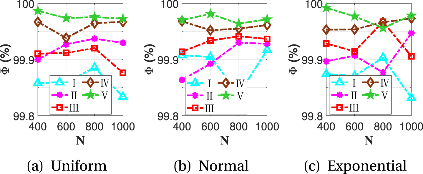
In order to show the time consumption of the four algorithms more clearly, Figures 11, 12, and 13 are based on the time consumption of PR and calculate the time efficiency improvement Φ between each other, that is $Φ = (t_{m} - t_{PR}) / t_{m} * 100 %$ (15) where t_PR is the time consumption of PR, and t_m is for other algorithms. It can be concluded from Fig. 11 that when the number of nodes is 400, the time consumption of PR is on average twice that of LC, and under the same constraint conditions, as the number of nodes continues to increase, the algorithm efficiency of PR has also been obtained. Increase, especially when the number of nodes is 1000, it can reach 85%. At the same time, as the constraints become more and more stringent (the value of |α_v - β_h| decrease gradually), this time efficiency has been better performed.

Fig. 11

Average time comparison (LC vs PR).

The comparison between the AC algorithm and the proposed algorithm is shown in Fig. 12. Due to the intelligent algorithms such as AC are solutions for very large networks, AC algorithms may be better than Pulse-R. While the heuristic methods improve the computational efficiency in large networks, the reduction percentage of the time between Pulse-R and AC fall slowly. Fig. 12 can show that when the number of nodes is less than 1000, the time consumed by the Pulse-R algorithm is reduced by more than 99% compared to the AC algorithm.

Fig. 12

Average time comparison (AC vs PR).

In Fig. 13, due to the existence of a heuristic search strategy, and the existence of a second inspection and correction process for feasible paths in PA, the time efficiency of PR is higher than that of PA when the same preprocessing and boundary strategies are used. This shows that the heuristic search strategy has a better effect than the PA rollback strategy.

Fig. 13

Average time comparison (PA vs PR)

To evaluate the convergence and convergence speed of the proposed heuristic, experiments were performed in a instances with a network node number of 600 and constraint III, compared with LC, PRW, PRP, PRB and PR.

The convergence curves of the six algorithms are illustrated in Fig. 14. Form these curves we can see that the best convergence rate belongs to the PR. The PRW has a poor convergence rate, and the convergence effect of PRP, PRB and LC are preferable but worse than the proposed algorithm. Moreover, it can be found by PRW that the solution space is huge when no pruning strategy is adopted, and although LC can quickly converge to the optimal solution, not quickly obtaining the feasible solution is its inadequacy.The convergence rate of PRP and PRB can conclude that the preprocessing and boundary strategies are effective, but there is a problem of insufficient efficiency in the late stage of search, while the incorporation of heuristic search strategy (PR) can avoid redundant search in the late stage and improve the efficiency of the algorithm.

Fig. 14

Comparative convergence curves of algorithms.

5 Discussion

The resource constrained shortest path problem with reinitilization has demonstrated its wider application in Smith [12]. Because there are resources to reinitiate the conditions, making the problem more complex while also expanding the search for viable solutions, the solution solving efficiency is tested.

Algorithms such as LC based on breadth first search (BFS) can be very effective in solving the shortest path problem, while its cost update on destination node is often at the end of the algorithm iteration, making the effect of some pruning strategies less obvious, such as the time consumption when the number of nodes is 1000 in Table 3. While due to the idea of DFS, PR, PA, etc. can combine the pruning strategy to delete redundant nodes, so that the efficiency of the algorithm can be greatly improved. It also shows that the efficiency of algorithms such as PR, PA is very dependent on the relevant pruning strategy.

PA has a better effect in larger scale networks [6], the reason for improving the boundary strategy is due to the large amount of computational time that needs to be consumed for the boundary calculation of this algorithm. Based on the idea of boundary pruning from the original algorithm and relaxing the constraints to obtain the lower boundary cost, the constraints on the lower boundary cost are less effective but the time consumed is significantly less compared with the traditional pulse algorithm. Meanwhile, the improved algorithm utilizes the heuristic search strategy of lower bound path to preorder the intended extended nodes, which can quickly exclude the nodes under increasing a certain memory demand, thus significantly improving the solving efficiency of the improved algorithm by up to 90%, compared with the original algorithm. At the same time, all of the improved algorithms have so elevated that they are largely based on boundary cost calculation, so how to obtain a better boundary cost while not significantly increasing the computational cost is a direction that needs to be studied in the future to improve the algorithms.

In summary, from the computational results, it was shown that the time consumption of PR did not significantly increase when the number of network nodes increased gradually, especially when the number of re-initialization nodes increases or the associated constraints are more stringent. Several pruning strategies and heuristic node expansion strategies are major contributions to this advantage. This study shows that improved algorithms are well suited to solve the problems.

6 Conclusion

In this paper, the UAV path planning problem with flight error correction is investigated, which can be modeled as RCSPP-R. The re-initiation condition of the resource expands the conventional feasible path set for constrained shortest path problems, increasing both the problem solving difficulty and the search cost. To solve such optimization problem, a heuristic algorithm (PR) based on PA [6] and branch bounds algorithm is proposed. In preprocessing, arcs and nodes that are not part of any feasible solution are removed by resource capacity and reinitiation constraints. The boundary clipping strategy reduces the redundant computation of the algorithm by calculating the effective lower boundary cost of relaxing the reinitiation constraint, and subsequently, the heuristic strategy preorders the extended nodes to improve the efficiency of the algorithm.

The instances are randomly generated by taking a similar approach to Smith [12], and the computational results show that the Pulse-R algorithm has a good performance of preprocessing and boundary pruning, with up to 99% and 97% of arcs and nodes can be removed with PRP and PRW, respectively. Compared with the pulse algorithm, the heuristic strategy based on the effective lower bound path, although increasing a certain degree of memory use but reducing the number of node extensions by up to 90%, greatly improves the time efficiency of the algorithm and the more obvious it is when the number of nodes of the network increases gradually. Through the experimental results with the label correction method, improved ant colony algorithm and pulse algorithm, etc., the proposed algorithm can solve the problem on the same scale in a shorter time, and the time efficiency can be improved up to 85.6% and 99%, respectively, which can provide a more effective solution in a network graph with thousands of nodes.

Footnotes

Acknowledgement

The authors would like to thank the editor and referees for their valuable comments and suggestions that help to improve this paper. This work is supported in part by Sichuan Science and Technology Program (No. 2021YJ0084) and the Research Project (G202012) of State Key Laboratory of Oil and Gas Reservoir Geology and Exploitation (Southwest Petroleum University).

References

Ajeil

F.H.

, Ibraheem

I.K.

, Azar

A.T.

and Humaidi

A.J.

, Grid-basedmobile robot path planning using aging-based ant colony optimizationalgorithm in static and dynamic environments, Sensors 20(7) (2020), 1880.

Cabral

E.A.

, Wide area telecommunication network design: Problems and solution algorithmswith application to the alberta supernet, 2005.

Ferone

, Festa

and Guerriero

, An efficient exact approachfor the constrained shortest path tour problem, OptimizationMethods and Software 35(1) (2020), 1–20.

Guo

and Liu

, Intelligent traffic cloud computing system based on ant colony algorithm, Journal of Intelligent & Fuzzy Systems, (Preprint) (2020), 1–12.

Laporte

and Pascoal

M.M.B.

, Minimumcost path problems withrelays, Computers and Operations Research 38(1) (2011), 165–173.

Lozano

, Duque

and Medaglia

A.L.

, An exact algorithmfor theelementary shortest path problem with resource constraints, Transportation Science 50(1) (2016), 348–357.

, Gong

L.-G.

and Yang

W.-L.

, An improved artificial bee colony algorithm based on balance-evolution strategy for unmanned combat aerial vehicle path planning, The ScientificWorld Journal, 2014, 2014.

Lozano

and Medaglia

A.L.

, On an exact method for the constrainedshortest path problem, Computers and Operations Research 40(1) (2013), 378–384.

, Pugliese

, Guerriero

and Poss

, The resourceconstrained shortest path problem with uncertain data: A robustformulation and optimal solution approach, Computers & Operations Research 107 (2019), 140–155.

10.

, Gai

, Zhang

and Zhong

, A novel hybrid grey wolfoptimizer algorithm for unmanned aerial vehicle (uav) path planning, Knowledge-Based Systems 194 (2020), 105530.

11.

Samir

, Sharafeddine

, Assi

C.M.

, Nguyen

T.M.

and Ghrayeb

, Uav trajectory planning for data collection from time-constrainediot devices, IEEE Transactions onWireless Communications 19(1) (2019), 34–46.

12.

Smith

O.J.

, Boland

and Waterer

, Solving shortest path problemswith a weight constraint and replenishment arcs, Computers andOperations Research 39(5) (2012), 964–984.

13.

Sujit

P.B.

, Saripalli

and Sousa

J.B.

, Unmanned aerial vehiclepath following: A survey and analysis of algorithms for fixed-wingunmanned aerial vehicless, IEEE Control Systems Magazine 34(1) (2014), 42–59.

14.

Tian

, Li

and Liu

, Robot global path planning using pso algorithmbased on the interaction mechanism between leaders and individuals, Journal of Intelligent & Fuzzy Systems, (Preprint) (2020), 1–9.

15.

Zhang

, Zhou

, Li

and Pan

, Grey wolf optimizer forunmanned combat aerial vehicle path planning, Advances inEngineering Software 99 (2016), 121–136.

16.

Zhang

, Song

, Shen

Z.-J.M.

and Wu

, Robust shortest pathproblem with distributional uncertainty, IEEE Transactions onIntelligent Transportation Systems 19(4) (2017), 1080–1090.

17.

Zhao

, Zheng

and Liu

, Survey oncomputational-intelligence-based uav path planning, Knowledge-Based Systems 158 (2018), 54–64.

18.

Zheng

, Luo

, Wang

and Chen

, Path planning of mobile robot based on adaptive ant colony algorithm, Journal of Intelligent & Fuzzy Systems, (Preprint) (2020), 1–10.