On the least amount of training data for a machine learning model

Abstract

Whether the exact amount of training data is enough for a specific task is an important question in machine learning, since it is always very expensive to label many data while insufficient data lead to underfitting. In this paper, the topic that what is the least amount of training data for a model is discussed from the perspective of sampling theorem. If the target function of supervised learning is taken as a multi-dimensional signal and the labeled data as samples, the training process can be regarded as the process of signal recovery. The main result is that the least amount of training data for a bandlimited task signal corresponds to a sampling rate which is larger than the Nyquist rate. Some numerical experiments are carried out to show the comparison between the learning process and the signal recovery, which demonstrates our result. Based on the equivalence between supervised learning and signal recovery, some spectral methods can be used to reveal underlying mechanisms of various supervised learning models, especially those “black-box” neural networks.

Keywords

Machine learning sampling theorem frequency principle signal recovery neural network Gaussian process regression

1 Introduction

Deep learning has made great achievements in various applications and became a hot topic in recent years [1 –6]. These achievements always can be attributed to the tremendous power of feature representation of deep neural networks (DNNs) [7], since according to the universal approximation theory, a DNN with enough nodes can arbitrarily approximate continuous functions in C (R^d) [8]. However, from a view of the classical theory in machine learning, a complex model is usually difficult to train and tends to generalize not well [9]. To overcome this problem, a larger amount of training data is needed. As a matter of fact, many achievements in recent years were made after big datasets were established, for example, ImageNet [10], which is a large-scale ontology of images built upon the backbone of the WordNet structure has boosted the development of computer vision.

Whether the exact amount of training data is enough for a specific task is an important question. On the one hand, it will lead to underfitting if the dataset is insufficient, where the data augmentation technique is always applied. On the other hand, it is always very expensive to label many data. For those tasks with big labeled datasets, it is not a problem. The commonly used scheme is to first project a DNN with many layers and nodes, then to train it with a big labeled dataset, next to prune or tune the network [11], until a satisfactory result is obtained. But for those lots of industry-specific tasks, labeled training data are always in short. So a key question is what the least amount of training data is for a machine learning network or model?

In this paper, we discuss this topic from the perspectives of sampling theorem and spectral-domain of a signal. If we take the target function of supervised learning as a multi-dimensional signal and the labeled data as samples, the training process can be regarded as a process of signal recovery. Then, the least amount of training data for a bandlimited task signal corresponds to a sampling rate that is larger than 2ω_M, i.e. the Nyquist rate, where ω_M is the cut-off frequency of the task signal.

The main highlights of this paper include:

(1) Novelty. As far as the authors’ knowledge, this is the first work to discuss the topic that what the least amount of training data is for a machine learning model. Moreover, an important phenomenon named Frequency Principle (F-Principle) [12] is explained in this paper theoretically from the perspective of the sampling theorem.

(2) Universality. The conclusion proposed in this work is not based on any specific network structures, activation functions, training methods, and training datasets. Since it views the target function as a high dimensional signal and analyzes the training process as a signal recovery process, the intermediate specific network structures, activation functions, and training methods are not restricted. In other words, the conclusion is valid for various supervised learning models, whether they are neural networks (NNs), SVM [13], or fuzzy systems [14 –16].

The remainder of this paper is organized as follows. In section 2, we introduce related works. In section 3, the sampling theorem and spectrum analysis of the training process of machine learning are discussed. Numerical experiments are shown in section 4. Some discussions are presented in section 5. Finally, in section 6, we summarize the concluding remarks and describe the future extension of this research work.

2 Related works

Spectral methods for neural networks. Studying neural networks by their spectral domains is not a new topic. Mathieu et al. [17] utilized spectral representations to accelerate computation in the learning process, while Sindhwani et al. [18] proposed structured transforms via Fast Fourier transform (FFT) to reduce the storage and memory requirements in deep networks. These ideas are very important in incremental machine learning or evolving intelligence, especially in online applications or mobile devices where various extended neural network frameworks are usually applied to fuzzy data streams [14] or missing values on data samples [15]. Spectral methods are also used to investigate the model robustness in computer vision [19], to study the generalization properties of gradient-based methods [20], or to act as a new regularization method to reduce network overfitting [21].

Spectral bias and Frequency Principle (F-Principle). By the usage of Fourier analysis, Rahaman et al. [22] found that deep networks prioritize learning the low frequency modes, a phenomenon they called spectral bias. Xu et al. [12] found a similar phenomenon empirically, which is referred to F-Principle: “a DNN with common settings first quickly captures the dominant low-frequency components, and then relatively slowly captures the high-frequency ones” [12]. The importance of the F-Principle was demonstrated by subsequent works. For example, Cai et al. [23] proposed a phase shift deep neural network which provides a wideband convergence in approximating a high dimensional function based on the fact that many DNN achieves convergence in the low frequency range first. Theoretical frameworks based on the F-Principle to study DNN training for multilayer networks with general activation functions, population densities of data, and a large class of loss functions are provided in Refs. [24, 25]. The universality of the F-Principle was demonstrated on high-dimensional benchmark datasets [26].

The aforementioned theoretical works on the F-Principle mainly concentrate on how to quantitatively characterize the spectral bias in a ReLU DNN [22] or how to rigorously investigate the F-Principle for the training dynamics of a general DNN at different training stages under some reasonable theoretical assumptions [24, 25]. However, an underlying theory to explain why the F-Principle holds, not how the F-Principle expresses, is still missing.

3 Sampling theorem and spectrum analysis of training process

3.1 The sampling theorem

The sampling theorem is pivotal in signal processing and its related application disciplines, which establishes the connection between continuous signals and discrete signals. It has various forms in the mathematics literature, such as the Whittaker-Kotelńikov-Shannon (or WSK) sampling theorem, the Nyquist sampling theorem, etc. A basic form is:

Theorem 1. [27] Let f (t) be a bandlimited signal with F (ω) =0 for |ω| > ω_M, F (ω) is the Fourier transform of f (t). Then f (t) is uniquely determined by its samples f (nT), n = 0, ± 1, ± 2, ⋯ if ω_s > 2ω_M, where $ω_{s} = \frac{2 π}{T}$ .

The sampling frequency ω_s is referred to as the Nyquist frequency while the frequency 2ω_M is commonly referred to as the Nyquist rate. For example, assume the target signal is $s (t) = sin (12 π t) + sin (6 π t) + sin (2 π t),$ (1) then ω_M is 6Hz and the Nyquist rate is 12Hz.

Theorem 1 indicates that a bandlimited signal can be recovered by its samples if the Nyquist frequency is larger than the Nyquist rate. Note that the sampled values f (nT) are given uniformly in Theorem 1. However, a similar result also holds for the nonuniform samples.

Theorem 2. [28]. If the average sampling rate of the nonuniform samples {t_n} is higher than the Nyquist rate, it can uniquely represent a band-limited signal (deterministic or random) if the samples are not the zero-crossings of a band-limited signal of the same bandwidth.

Theorems 1 and 2 are all for the 1-D signals. Multi-dimensional signals can also be recovered by their samples under some assumptions, the readers can refer to Ref. [28].

3.2 Supervised learning training versus signal recovery

In this paper, only the supervised learning is considered. Practically, supervised learning is to learn a function from the input data space Rⁿ to the output data space R^m. Usually, some specific network and training methods are chosen to fit the labeled data. For example, in the kernel machines [29] such as SVM [13], the input data and their corresponding output are used to determine the coefficients of kernels, of which the network is the SVM model, and the training method can be chosen the stochastic gradient descent algorithm [30]. Similarly, in deep learning, the labeled data are used to determine the parameters of DNN or CNN, while the network is DNN/CNN, and the training method is usually the gradient descent algorithm or some numerical algorithm like Levenberg-Marquardt (LM) backpropagation method [31].

If we take the target function as a multi-dimensional signal and the labeled data as samples, the training process can be regarded as a process of signal recovery. The samples are given nonuniformly. In this sense, it is natural to explain the training process of machine learning from the perspective of the sampling theorem:

The training process of supervised learning is a process of signal recovery. According to the sampling theorem, if the information of f at its frequency ω needs to be recovered, the amount of 2ω samples needs to be provided. By contrast, with more and more discrete samples are provided, the information of higher and higher frequencies can be extracted. Changed to the words of machine learning, with more and more labeled data are learned, components of the target function are captured from low-frequency to relatively high-frequency. This is just the phenomenon of the F-Principle. A comparative diagram between the learning process and the signal recovery is illustrated in Fig. 1. Meanwhile, it suggests the least amount of training data for a bandlimited task signal corresponds to a sampling rate that is larger than the Nyquist rate.

Fig. 1

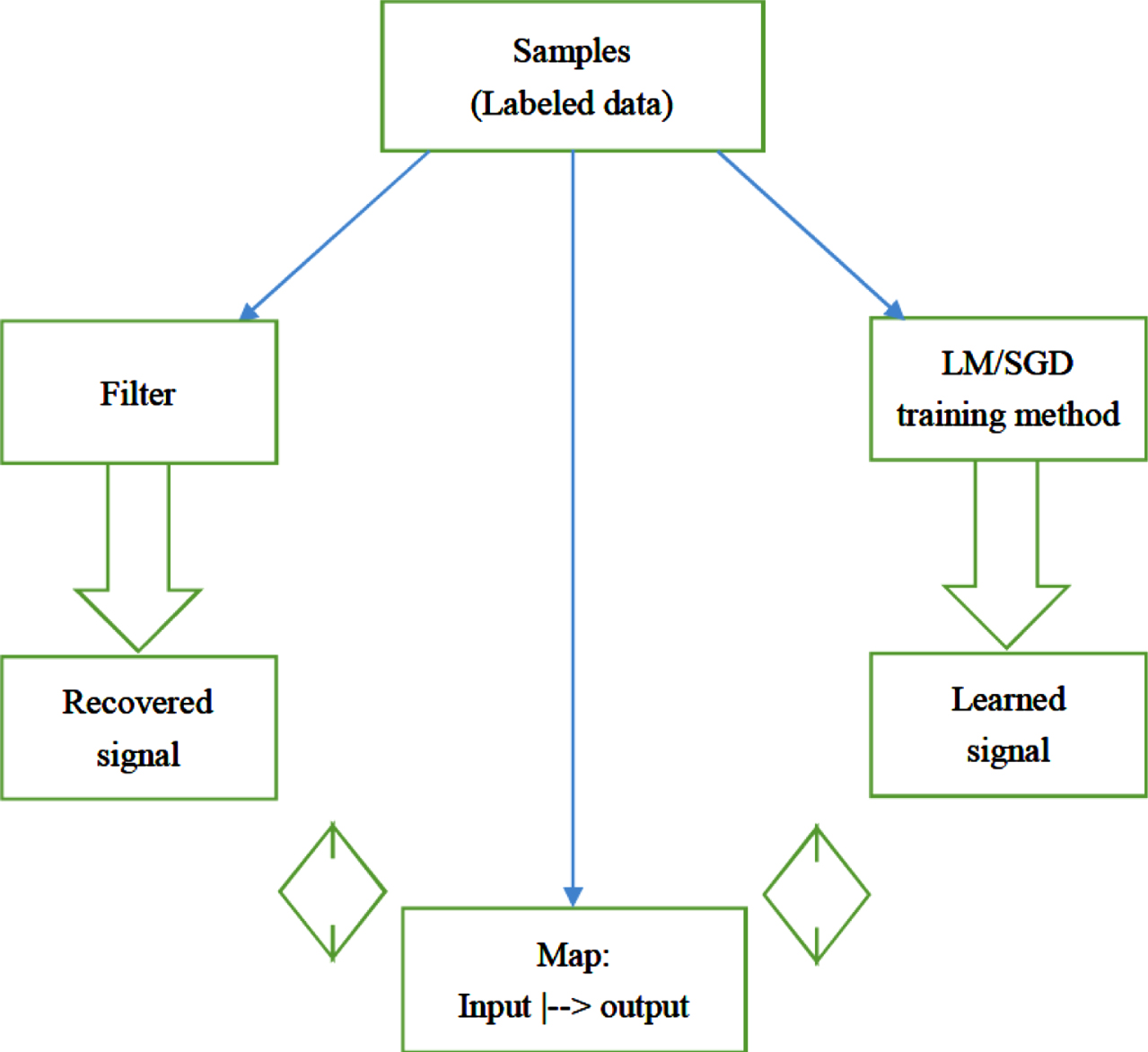
A comparison of signal recovery with supervised learning training.

In the next section, we will give some examples and experiments to show the equivalence between the process of supervised learning training and the process of signal recovery.

Fig. 2

A signal with 4 different sampling rates. (a): Signals in the time domain. (b): Signals in the frequency domain.

Fig. 3

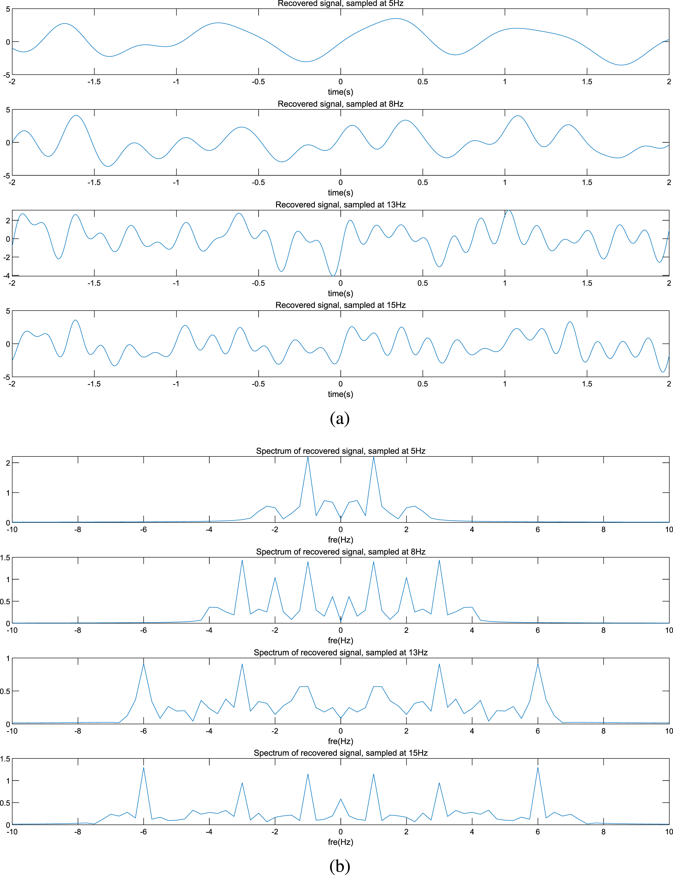
Recovered signals and their spectrums. (a) The signals recovered by passing through lower pass filters. (b) Spectrums of the recovered signals.

Fig. 4

Signals learned by the NN and their spectrums. (a) Signals learned by the NN. (b) Spectrums of the signals learned by the NN.

Fig. 5

Average signals learned by the NN and their spectrums. (a) Average signals learned by the NN. (b) Spectrums of the average signals learned by the NN.

Fig. 6

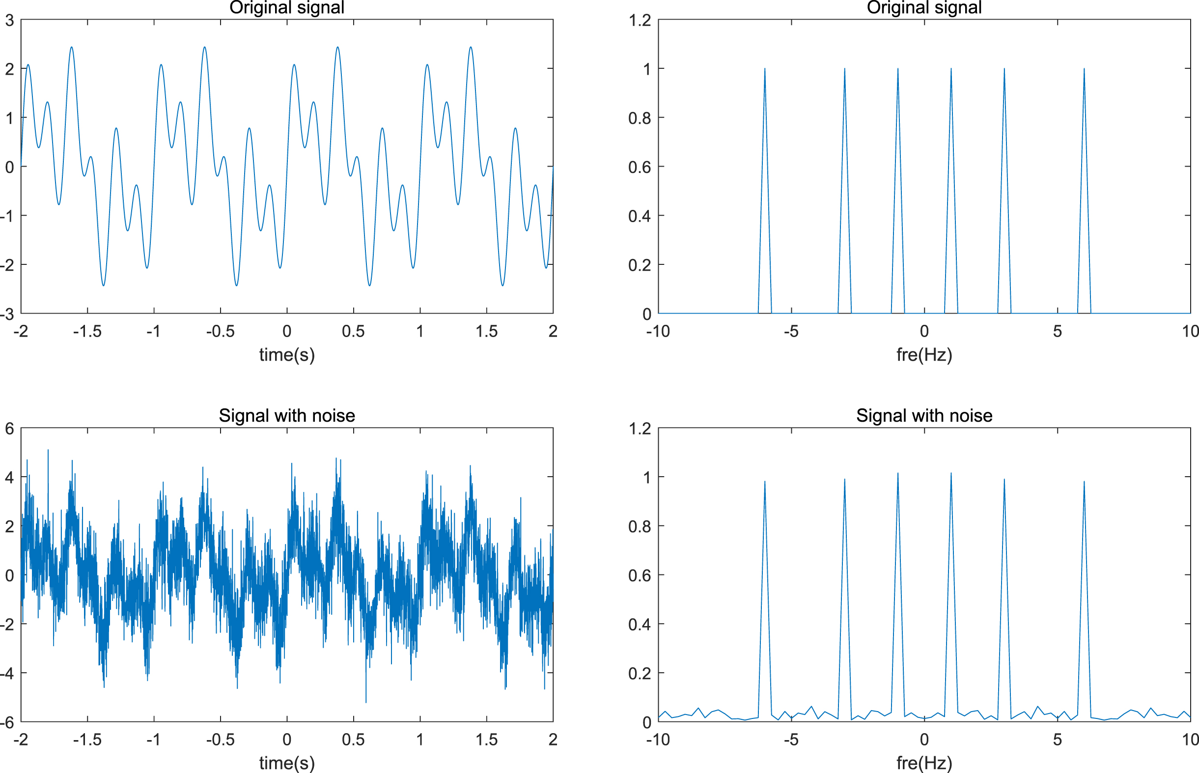
A signal with white noise. Left: the signal in the time domain. Right: the signal in the frequency domain.

4 Experiments

4.1 The one-dimensional signal recovery and the neural network learning

I. without noise.

The target signal is $s (t) = sin (12 π t) + sin (6 π t) + sin (2 π t) .$ (2) Obviously, s (t) is composed with 3 frequencies: 1Hz, 3Hz, 6Hz. According to the sampling theorem, the sampling rate should be larger than 12Hz if we want to recover s (t) without information lost. Let s (t) be sampled by the rates of 5Hz, 8Hz, 13Hz and 15Hz respectively. The corresponding signals and their spectrum are shown in Fig. 2. It is noted that the y-axis denotes the amplitude of the signal while the x-axis can denote time or frequency. This illustration applies to all the following 2D graphics, and it is similar to 3D graphics.

The recovered signals and their spectrums are shown in Fig. 3(a) and (b), where signals are recovered by passing through lower pass filters [27]. When the sampling rate is 5Hz, only the component of 1Hz of s (t) is recovered. Meanwhile, an aliasing component of 2Hz is watched. This indicates that s (t) can not be recovered from the samples generated by the sampling rate of 5Hz since all the frequencies higher than 2.5Hz are lost and an aliasing component is made incorrectly. It is a similar case when the sampling rate is 8Hz: the components of 1Hz and 3Hz are recovered while the component of 6Hz is lost and an aliasing component of 2Hz is made. When the sampling rates are 13Hz and 15Hz, s (t) is recovered completely since these two sampling rates are larger than the Nyquist rate.

The sampling theorem provides a theoretical requirement of how to recover a signal by its samples. Correspondingly, machine learning methods provide concrete ways to recover the signal.

Establish a 1 × 100 × 1 neural network, and the training data are sampled by the rates of 5Hz, 8Hz, 13Hz, and 15Hz respectively. Parameters are set as: the learning rate lr = 0.002, the max epochs times = 30000 and the error target goal = 0.001. The training is implemented by the LM backpropagation method. Figure 4 shows signals learned by the neural network and spectrums of the signals respectively.

Compared with Fig. 3(b), it is noted that the signals learned by the neural network are nearly the same as the signals recovered by passing through lower pass filters. When the sampling rate is 5Hz, the components of 1Hz and 2Hz of s (t) are learned apparently, of which the 2Hz component is a faked frequency. Meanwhile, some frequencies lower than 4Hz are also learned, but they are also faked. When the sampling rate becomes larger and larger, that is, when the training data set becomes larger and larger, the components of 1Hz, 3Hz, and 6Hz are all learned while those faked lower frequencies disappear or become to nearly zero.

Fig. 7

Recovered signals with different sampling rates and their spectrums, the original signal is mixed with white noise. (a) Recovered signals. (b) Spectrums of the recovered signals.

Since the initial parameters of the neural network are set randomly, we may wonder whether the learning results vary heavily at different simulations. Take the average signal of 3 times simulations as the output signal. Figure 5 displays the average signals in the time domain and their corresponding spectrums. It seems the results are nearly not affected by the initial random parameters.

This example in fact shows the equivalence between supervised learning of NN and signal recovery. Note that we employ the LM backpropagation method for NN training here, which is essentially a numerical training method. If we replace it with the standard backpropagation (BP) algorithm, we will find that it is difficult to learn the 6Hz component of the signal even if the sampling rate is 13Hz. This indicates that the least amount of training data we consider here is a theoretical guarantee, which does not suggest that the function can be learned with the least amount of training data by using a training method casually. It also shows that the numerical training methods like the LM algorithm are more effective when the samples dataset is relatively small.

Fig. 8

Signals learned by the NN and their spectrums, data are mixed with white noise. (a) Signals learned by the NN. (b) Spectrums of the signals learned by the NN.

II. with noise.

Data used in machine learning are always contaminated by various noises. In order to investigate the effect of noise, we examine the signal recovery and neural networks learning with noise. The gaussian white noise is adopted, where the standard deviation is σ = 1, as shown in Fig. 6.

The recovered signals and their spectrums are shown in Fig. 7(a) and (b), where the signals are recovered by passing through lower pass filters. Comparing Figs. 3(b) and 7(b), we notice that spectrums of 7(b) have non-zero amplitudes at nearly all the frequencies. It is because the spectrum of white noise is infinite theoretically.

Comparatively, the signals learned by neural networks trained with noisy data, and their spectrums are shown in Fig. 8(a) and (b). It is obvious that the learning results are affected by the noise since learned signals are distorted a little, however, the “real” frequencies of 1Hz, 3Hz and 6Hz can be recognized apparently. When the noise is heavy enough, that is σ is large enough, it is difficult to recover the signal or learn the signal from noisy training data.

Fig. 9

The 2-D signal and its spectrum. (a) The 2-D signal. (b) Spectrum of the signal.

4.2 The high dimensional signal recovery and the neural network learning

In practical tasks, the input data are always multi-dimensional. Similar to the one-dimensional signal recovery and the neural network learning experiments, we examine the case of two-dimensional signal recovery.

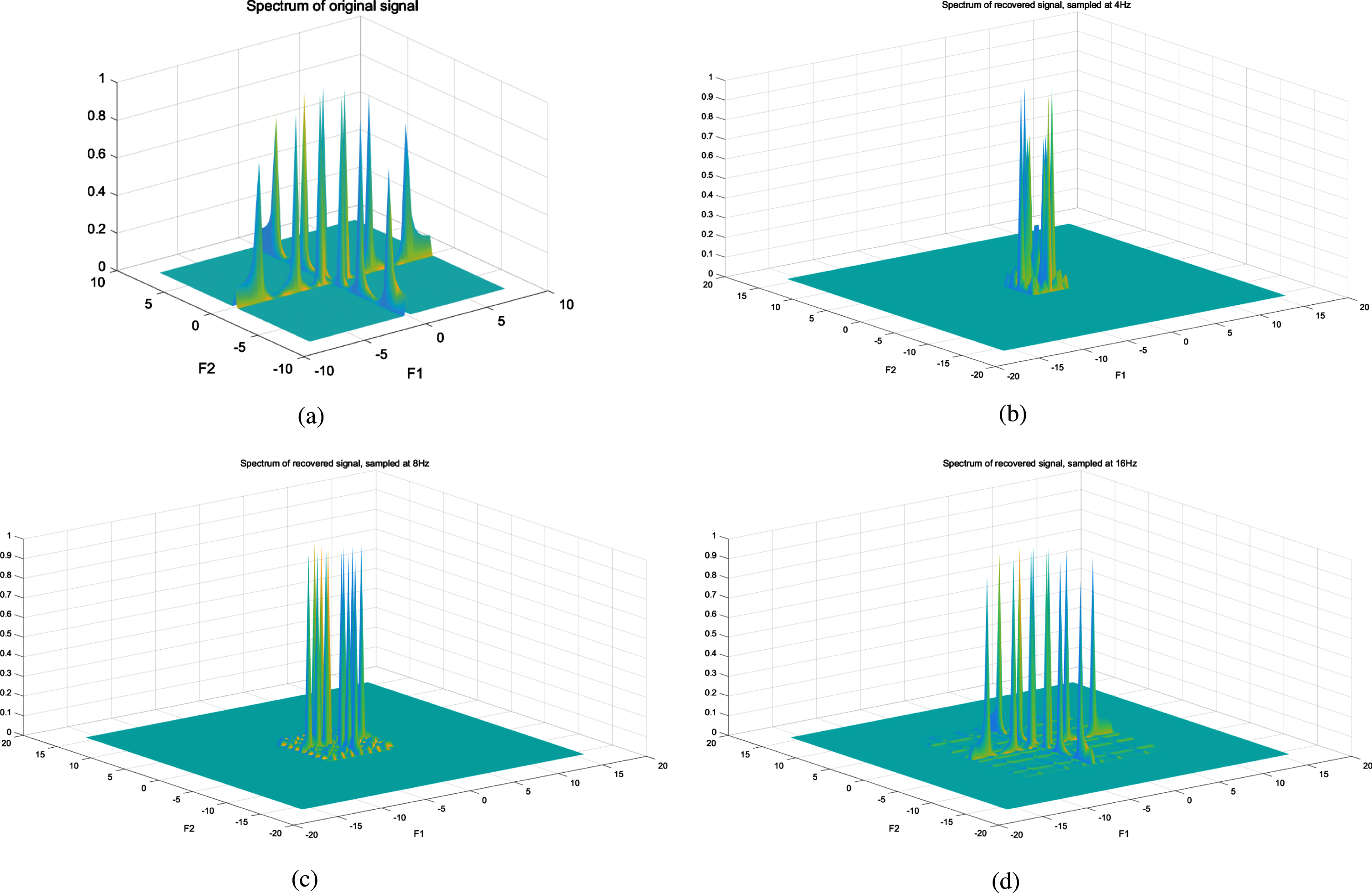
The target signal is $\begin{matrix} s (x, y) & = & sin (12 π x) + sin (6 π x) + sin (2 π x) \\ + & sin (12 π y) + sin (6 π y) + sin (2 π y) . \end{matrix}$ Obviously, s (x, y) is composed with 3 frequencies: 1Hz, 3Hz, 6Hz in both the x-direction and the y-direction. According to the Nyquist sampling theorem, the sampling rate should be larger than 12Hz if we want to recover s (x, y) without information lost. In order to apply the FFT operations directly, we make s (t) be sampled by the rates of 4Hz, 8Hz, and 16Hz respectively. The corresponding signals and their spectrum are shown in Fig. 9. Figure 9(b) display the obvious 6 peaks of the spectrum: (1, 0) , (0, 1) , (3, 0) , (0, 3) , (6, 0) and (0, 6).

Fig. 10

Spectrums of the recovered signals, where signals are recovered by passing through lower pass filters. (a) Spectrum of the original signal. (b) Sampling rate is 4Hz. (c) Sampling rate is 8Hz. (d) Sampling rate is 16Hz.

Figure 10 displays the recovered signals and their spectrums, where signals are recovered by passing through lower pass filters, the sampling rates are 4Hz, 8Hz, and 16Hz respectively. Figure 10(b) shows 6 peaks of the spectrum: (0, 1) , (1, 0) , (0, 1.75) , (1.75, 0), (0, 0.25) , (0.25, 0). The component of frequency 1Hz is recovered when the sampling rate is 4Hz. However, the aliasing components of 0.25Hz and 1.75Hz also appear. This phenomenon is consistent with the sampling theorem. When the sampling rate turns to 8Hz, components of 1Hz and 3Hz are recovered while an aliasing 2Hz appears. Finally, when the sampling rate is 16Hz, all the three components are recovered and there are no aliasing frequencies.

Assume s (t) has N training samples at some sampling rate, then s (x, y) has N² training samples at the same rate. So we need a larger neural network to train samples of s (x, y). Establish a 1 × 550 × 1 neural network, and the training data are sampled by the rates of 4Hz, 8Hz and 16Hz respectively. Other parameters are the same as the neural network for s (t) in Equation (2).

Figure 11 shows spectrums of the signals learned by the neural network. When the sampling rate is 4Hz, only the low frequencies are learned, where the peak point is at (0, 0). Amplitudes of the ideal components (0, 1) and (1, 0) are about 0.1. When the sampling rate gets larger, more frequencies are learned. However, Fig. 11(b) and (c) tell us the training processes are not convergent at low sampling rates. When the rate turns to 16Hz, all the ideal components are learned. Figure 11(d) shows 3-class apparent peaks: amplitudes at (0, 1) and (1, 0) are 1 while amplitudes at (0, 3) and (3, 0) are 0.8594 and amplitudes at (0, 6) and (6, 0) are 0.3577.

Fig. 11

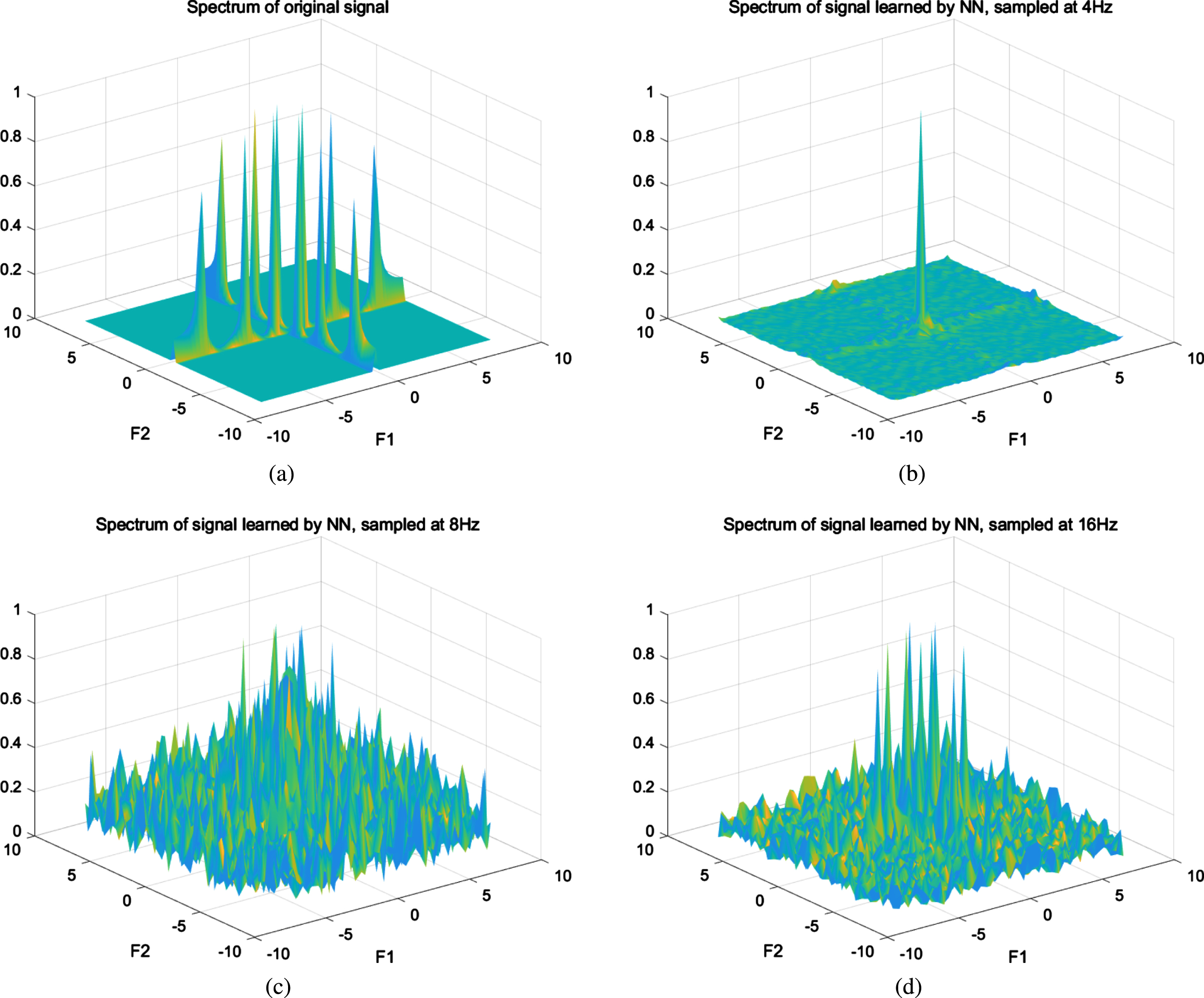
Spectrums of the signals learned by NN. (a) Spectrum of the original signal. (b) Sampling rate is 4Hz. (c) Sampling rate is 8Hz. (d) Sampling rate is 16Hz.

4.3 The one-dimensional signal recovery and the Gaussian process regression

The Gaussian process regression (GPR) is a known machine learning method for regression tasks, which is mathematically equivalent to or closely related to many well known models under suitable conditions, including large neural networks and SVMs [32].

The target signal is also $s (t) = sin (12 π t) + sin (6 π t) + sin (2 π t) .$ The main parameters used in the GPR experiment is listed in Table 1.

Table 1
Main parameters of GPR

Basis function Kernel function Optimizer

Constant Exponential L-BFGS [33]

Basis function	Kernel function	Optimizer
Constant	Exponential	L-BFGS [33]

The signals learned by the GPR and their spectrums are shown in Fig. 12 (a) and (b). Similar to Fig. 8, the components of 1Hz, 3Hz, and 6Hz are all learned correctly when the training dataset becomes larger and larger. However, when the sampling rates are 5Hz and 13Hz, the amplitudes of recovered signals are very small while the amplitudes increase to normal levels when the sampling rate is larger than 15Hz. This example also indicates that the least amount of training data we consider here is a theoretical lower bound, which is not enough for the GPR method. Meanwhile, the parameter setting will affect the results even if the training dataset remains the same. For example, if the kernel function in Table 1 is replaced by a rational quadratic function, more training data are required for the same precision level of the recovered signal.

Fig. 12

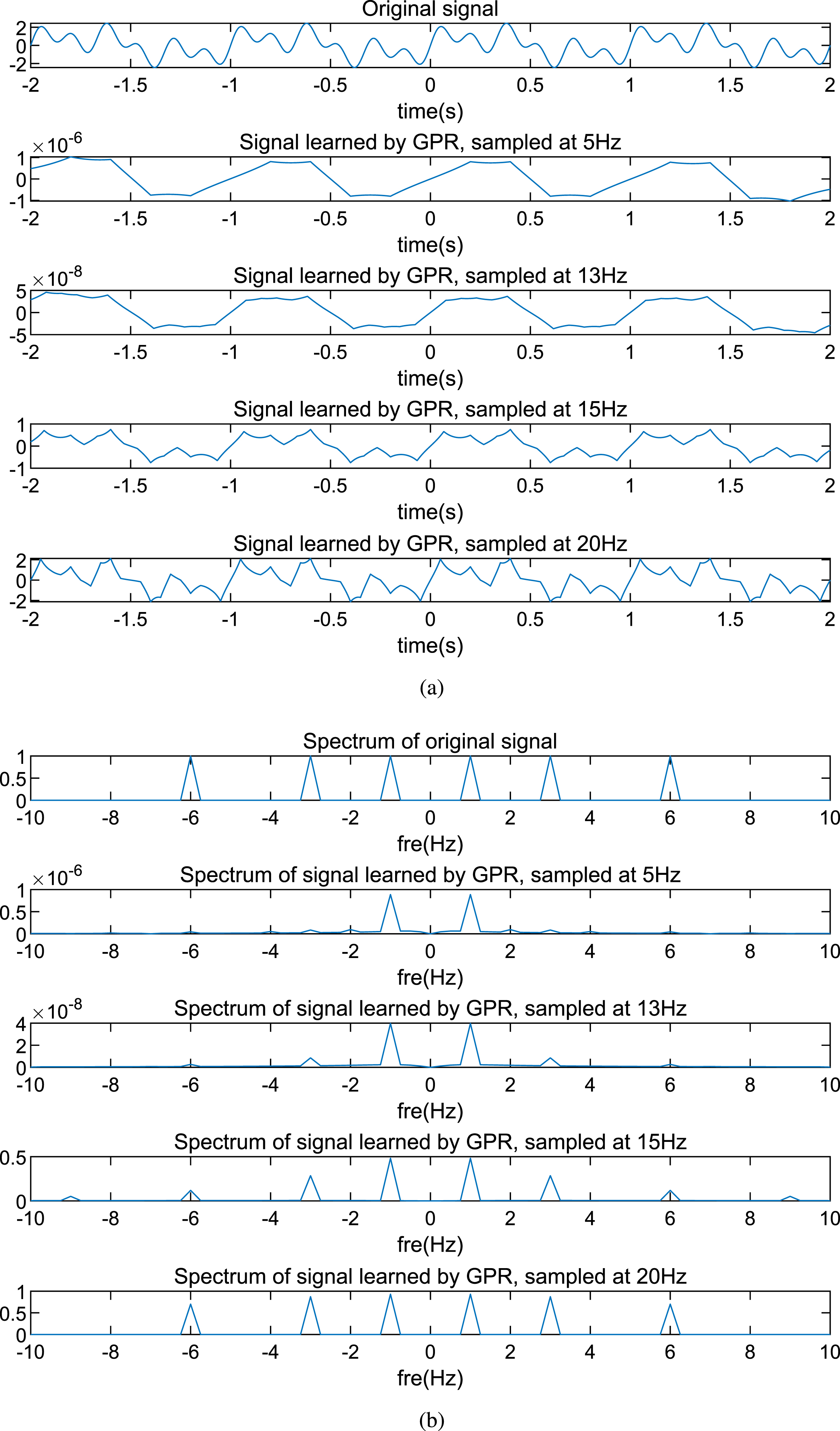
Signals learned by the GPR and their spectrums. (a) Signals learned by the GPR. (b) Spectrums of the signals learned by the GPR.

5 Discussions

I. What is the inspiration of sampling theorem for machine learning?

Experiments in section. 4 prove the high consistence between the signal recovery with sampling theorem and the supervised learning process. This fact inspires us to study machine learning with the help of signal processing methods and means, such as spectral analysis, time-frequency analysis and so on. Specifically, we can investigate the different stages of learning process with various initial data, learning models, and initial parameters. The aforementioned works on the F-Principle belong to this kind. Moreover, we can further apply the spectral analysis methods of signal processing to the influences of regularization methods, dropout operations [34], and so on.

II. Why do not we utilize the lower pass filter to substitute the machine learning methods?

Although the above experiments indicate that making the samples passing through a lower pass filter and training the samples both come to similar results, these two methods are different. On the one hand, the dimension of data for machine learning is usually far high than signal processing, then designing an appropriate filter for a high-dimensional signal is a difficult task. Meanwhile, the spectral analysis of high-dimensional signals requires huge computational costs. On the other hand, the current machine learning methods are already effective, and there exist many open-source frameworks to support these methods. However, although we do not utilize the lower pass filter to substitute the machine learning methods, investigating machine learning with the help of signal processing methods and means will provide a new perspective for the study of the internal mechanism of machine learning, and new ideas and inspiration for the design of new training methods and regularization methods.

6 Conclusion and future work

In this paper, we discuss the topic that what is the least amount of training data for a model from the perspective of the sampling theorem. If we take the target function of supervised learning as a multi-dimensional signal and the labeled data as samples, the training process can be regarded as a process of signal recovery. The main result is that the least amount of training data for a bandlimited task signal corresponds to a sampling rate which is larger than the Nyquist rate. Some numerical experiments are carried out to show the comparison between the learning process and signal recovery, which demonstrates the equivalence between the supervised learning and the signal recovery.

Although the spectral methods are not appropriate to apply to high-dimensional signals due to the costly computations, we can use them to reveal some underlying mechanisms of various supervised learning models, whether they are NN, kernel models, or fuzzy systems, especially those “black-box” NNs. For example, we can investigate how the influences of regularization methods act in the process of learning from the perspective of frequency domain. On the contrary, we can design new training methods and regularization methods based on the previous spectral analysis results.

Footnotes

Acknowledgments

The authors are very grateful to the reviewers for their comments and suggestions which have improved the paper. This work was supported in part by the Sichuan Science and Technology Program (No. 2021YJ0526 and No. 2022NSFSC1840), the open fund of Sichuan National Applied Mathematics Center (No. 2022-KFJJ-01-002), and the Exploration Project of Zhejiang Natural Science Foundation (No. LQ20G010004).

Conflict of interest

The authors declare that there is no conflict of interest regarding the publication of the paper.

References

Krizhevsky

, Sutskever

, Hinton

. Imagenet classification with deep convolutional neural networks, In, Advances in Neural Information Processing Systems, 2012, 1097–1105.

LeCun

, Bengio

, Hinton

. Deep learning, Nature 521 2015, 436–444.

, Zhang

, Ren

, Sun

. Deep residual learning for image recognition, In Proceedings of the IEEE Conference on Computer Vision and Pattern Recognition, 2016, 770–778.

Silver

, Huang

, Maddison

et al. Mastering the game of go with deep neural networks and tree search, Nature 529 2016, 484–489.

Zhao

, Yu

, Li

. Diffusion on Fractal Objects Modeling and its Physics-Informed Neural Network Solution, Fractals 29(3) 2021, 2150071.

Punia

S.K.

, Kumar

, Stephan

, Deverajan

G.G.

, Patan

. Performance analysis of machine learning algorithms for big data classification: Ml and ai-based algorithms for big data analysis, International Journal of E-Health and Medical Communications 12(4) 2021, 60–75.

Zhao

, Yu

, Xu

, Luo

. Equivalence between dropout and data augmentation: A mathematical check, Neural Networks 115 2019, 82–89.

Pinkus

. Approximation theory of the MLP model in neural networks, Acta numerica 8 1999, 143–195.

Shalev-Shwartz

, Ben-David

. Understanding Machine Learning: From Theory to Algorithms, Cambridge University Press, New York, NY, USA, 2014.

10.

Deng

, Dong

, Socher

, Li

L.J.

, Li

. Imagenet: A large-scale hierarchical image database, In IEEE Conference on Computer Vision and Pattern Eecognition, 2009, pp. 248–255.

11.

Montavon

, Orr

, Mĺźller

K.R.

. Neural networks: tricks of the trade, Springer-Verlag, Berlin, Heidelberg, 2012.

12.

Z.Q.J.

, Zhang

, Xiao

. Training behavior of deep neural network in frequency domain, arXiv preprint arXiv:1807.01251, 2018.

13.

Vapnik

. The nature of statistical learning theory, Springer Science & Business Media, New York, 2000.

14.

Leite

, Costa

, Gomide

. Evolving granular neural networks from fuzzy data streams, Neural Networks 38 2013, 1–16.

15.

Garcia

, Leite

, Škrjanc

. Skrjanc, Incremental missing-data imputation for evolving fuzzy granular prediction, IEEE Transactions on Fuzzy Systems 28(10) 2019, 2348–2362.

16.

Janarthanan

, Maheshwari

R.U.

, Shukla

P.K.

, Shukla

P.K.

, Mirjalili

, Kumar

. Intelligent Detection of the PV Faults Based on Artificial Neural Network and Type 2 Fuzzy Systems, Energies 14(20) 2013, 6584.

17.

Mathieu

, Henaff

, LeCun

. Fast training of convolutional networks through FFTs, In International Conference on Learning Representations, 2014.

18.

Sindhwani

, Sainath

, Kumar

. Structured transforms for small-footprint deep learning, In Advances in Neural Information Processing Systems, 2015, pp. 3088—3096.

19.

Yin

, Lopes

R.G.

, Shlens

, Cubuk

E.D.

, Gilmer

. A fourier perspective on model robustness in computer vision, arXiv preprint arXiv:1906.08988, 2019.

20.

Farnia

, Zhang

J.M.

, David

N.T.

. A Fourier-based approach to generalization and optimization in deep learning, IEEE Journal on Selected Areas in Information Theory 1 2020, 145–156.

21.

Khan

S.H.

, Hayat

, Porikli

. Regularization of deep neural networks with spectral dropout, Neural Networks 110 2019, 82–90.

22.

Rahaman

, Baratin

, Arpit

, et al. On the spectral bias of neural networks, In International Conference on Machine Learning, 2019, pp. 5301—5310.

23.

Cai

, Li

, Liu

. Phasednn–a parallel phase shift deep neural network for adaptive wideband learning, arXiv preprint arXiv:1905.01389, 2019.

24.

Z.Q.J.

. Understanding training and generalization in deep learning by fourier analysis, arXiv preprint arXiv:1808.04295, 2018.

25.

Luo

, Ma

, Xu

Z.Q.J.

, Zhang

. Theory of the frequency principle for general deep neural networks, arXiv preprint arXiv:1906.09235, 2019.

26.

Z.Q.J.

, Zhang

, Xiao

, Ma

. Frequency principle: Fourier analysis sheds light on deep neural networks, arXiv preprint arXiv:1901.06523, 2019.

27.

Oppenheim

A.V.

, Willsky

A.S.

, Nawab

S.H.

. Signals and systems, vol. 2, Prentice-Hall Englewood Cliffs, NJ, 1983.

28.

Marvasti

. Nonuniform Sampling: Theory and Practice, Springer Science & Business Media, New York, 2001.

29.

Schölkopf

, Smola

A.J.

. Learning with kernels: support vector machines, regularization, optimization, and beyond, MIT Press, Cambridge/London, 2002.

30.

Shalev-Shwartz

, Singer

, Srebro

, Cotter

. Pegasos: Primal estimated sub-gradient solver for svm, Mathematical programming 127 2011, 3–30.

31.

Levenberg

. A method for the solution of certain non-linear problems in least squares, Quarterly of applied mathematics 2 1944, 164–168.

32.

Williams

C.K.

, Rasmussen

C.E.

. Gaussian processes for machine learning, MIT Press, Cambridge, MA, USA, 2006.

33.

Liu

D.C.

, Nocedal

. On the limited memory BFGS method for large scale optimization, Mathematical programming 45(1) 1989, 503–528.

34.

Hinton

G.E.

, Srivastava

, Krizhevsky

, Sutskever

, Salakhutdinov

R.R.

. Improving neural networks by preventing co-adaptation of feature detectors, arXiv preprint arXiv:1207.0580, 2012.

On the least amount of training data for a machine learning model

Abstract

Keywords

1 Introduction

2 Related works

3 Sampling theorem and spectrum analysis of training process

3.1 The sampling theorem

4.1 The one-dimensional signal recovery and the neural network learning

Table 1 Main parameters of GPR Basis function Kernel function Optimizer Constant Exponential L-BFGS [33]

6 Conclusion and future work

Footnotes

Acknowledgments

Conflict of interest

References

Table 1
Main parameters of GPR

Basis function Kernel function Optimizer

Constant Exponential L-BFGS [33]