Forecasting public bicycle rental demand using an optimized eXtreme Gradient Boosting model

Abstract

The rational distribution of public bicycle rental fleets is crucial for improving the efficiency of public bicycle programs. The accurate prediction of the demand for public bicycles is critical to improve bicycle utilization. To overcome the shortcomings of traditional algorithms such as low prediction accuracy and poor stability, using the 2011–2012 hourly bicycle rental data provided by the Washington City Bicycle Rental System, this study aims to develop an optimized and innovative public bicycle demand forecasting model based on grid search and eXtreme Gradient Boosting (XGBoost) algorithm. First, the feature ranking method based on machine learning models is used to analyze feature importance on the original data. In addition, a public bicycle demand forecast model is established based on important factors affecting bicycle utilization. Finally, to predict bicycle demand accurately, this study optimizes the model parameters through a grid search (GS) algorithm and builds a new prediction model based on the optimal parameters. The results show that the optimized XGBoost model based on the grid search algorithm can predict the bicycle demand more accurately than other models. The optimized model has an R-Squared of 0.947, and a root mean squared logarithmic error of 0.495. The results can be used for the effective management and reasonable dispatch of public bicycles.

Keywords

Bicycle demand forecast feature importance grid search algorithm optimal parameters eXtreme Gradient Boosting

1 Introduction

The shared bicycles will gradually become an important part of the urban public transportation system as a green, low-carbon and healthy travel mode. The rapid development of shared bicycles has played a key role in satisfying public travel, reducing air pollution, and alleviating traffic pressure, and can be used as a connecting tool for conventional buses and subways to expand the scope of urban public transportation services [1]. At present, the most popular public bicycle systems use “pile-free” shared bicycles [2], this kind of bicycle has no fixed docking station, which is more convenient for cyclists. However, in the development process of the public bicycle system, there are also problems such as unreasonable allocation and resource scheduling, which affects the reasonable operation and management of shared bicycles [3]. The demand for public bicycles is different in different time periods. Accurate prediction of the demand for rentals allows public bicycle systems to avoid shortages peak commuting times to improve utilization rates, so that public bicycles better serve the public. Therefore, the forecast of demand for public bicycles can provide an important basis for the dispatch and management of urban public bicycle resources [4].

Through the mining and analysis of historical data, it is a core problem that needs to be solved to accurately and efficiently predict the demand for public bicycles. Many scholars have devoted themselves to predicting the demand for public bicycles [5 –9]. Traditional statistical models and linear models were widely used to estimate bicycle demand in a certain area [10]. Barnes et al. [11] estimated the possible range of total bicycle demand in a certain area based on census commuting data, this method mainly obtains data through manual investigation, which is time-consuming and labor-intensive, and the collected raw data is limited. Singhvi et al. [12]. used a linear regression model to predict the demand for bicycles at stations in New York City. Zhang et al. [13] proposed two prediction models based on MART regression and Lasso regression, which respectively predicted the final destination and the duration of use bicycle. Zhang et al. [14] used the historical user data of the public bicycle system in Zhongshan City, and used a multiple linear regression model to study the impact of various scenic spots on travel demand and the ratio of station demand to supply in Zhongshan City. Juan et al. [15] used Bayesian network and analysed bicycle demand based on vehicle factors, load factors, environmental factors and human factors. To accurately adapt to seasonal changes in bicycle demand, Fournier et al. [16] proposed a sine model to estimate bicycle demand. The model can estimate the monthly average daily bicycle count and the annual average daily bicycle count. Zhang et al. [17] established a linear regression model. The model reflects the relationship between the demand for public bicycle rental and the characteristics of land use within the scope of the rental station. Ryu et al. [18] used the O-D matrix method to estimate the bicycle demand in a small community. This method is not suitable for processing data with a large amount of calculation.

The above researches use relatively simple algorithms to estimate bicycle demand, and have low utilization of raw data. There are many factors that affect the demand for bicycles. The studies of Bd et al. [19] and Chibwe et al. [20] have shown that location, facility type, meteorological, Unemployment rate, temperature, rainfall, wind speed, household income and other factors will affect the change in bicycle demand. This means that bicycle demand forecasting models need to consider more factor, and explores the relationship between these factors and the bicycle demand. Traditional models cannot reveal the complex relationships among multiple feature factors, and the prediction performance of these methods depends on the quality of the data.

With the rapid development of artificial intelligence, more and more scholars are committed to studying the application of machine learning algorithms in bicycle demand forecast. Martins et al. [21] used a random forest model to predict bicycle demand for public stations in Barcelona and add weather forecast information to improve the prediction accuracy of the model. Chen et al. [22] used the BP neural network model to predict the number of bicycle rentals at bicycle rental sites. The predicted value and the actual value differ by about 3 vehicles on average, and the curve fits well, which proves that the model can be practical. In order to accurately predict the usage information of users in public bicycle systems from massive data, Feng et al. [23] used multiple linear regression model to predict bicycle demand but do not achieve sufficient predictive accuracy. Therefore, the authors estimate a random forest model using the same data. The results show that the random forest prediction is better than the multiple linear regression model. Kang Z et al. [24] combined user behavior, weather, and holiday data from Citi Bike and estimate multiple regression, decision tree, and random forest models. The highlights of the article are the richness of the data and the comparative analysis of the three different models. In order to plan the efficient distribution of public bicycles between sites, Yao X et al. [25] proposed a public bicycle demand forecasting method based on space-time correlation. The method analysed the use of the bicycle sharing system based on long-term stability and short-term volatility. The method considers the user’s demand from both the time and space perspectives, to schedule the bicycle more efficiently. Gao et al. [26] proposed a method for predicting bicycle demand based on Fuzzy C-Mean (FCM) Genetic Algorithm (GA) and Back Propagation Network (BPN), the root mean squared error (RMSE) and mean absolute error (MAE) are used to evaluate case analysis results to verify the effectiveness of the model. The results show that the proposed method can effectively forecast demand.Yi Ai et al. [27] adopted a deep learning method, named the convolutional long short-term memory network (conv-LSTM), to solve spatial and temporal dependencies. Experiments show that conv-LSTM is better than LSTM in capturing space-time correlation. This method is innovative and takes into account the dynamic characteristics of the public bicycle system to a certain extent. Xu et al. [28] proposed a dynamic scheduling (DBS) model based on short-term demand forecasting. The method first uses K-means to cluster the sites, and uses random forest (RF) to predict the demand for bicycles in each category. Finally, the performance of the model is evaluated through the data set from the Chicago Public Bicycle Sharing System, and the root mean squared logarithmic error (RMSLE) indicator is used to evaluate the model prediction results. Chen et al. [29] used recurrent neural networks to predict the demand for public bicycles, and four indicators, mean absolute percentage error (MAPE), RMSLE, MAE and RMSE, are used to evaluate the performance of the model. Seo et al. [30] adopted random forest machine learning technology for demand forecasting. The case study used the public bike-sharing (PBS) database in Seoul, South Korea, and the RMSE indicator was used to evaluate the performance of the random forest model. Li et al. [31] transformed the original time series data into high-order tensor time series, and proposed a city public bicycle prediction model based on the HOSVD-LSTM hybrid algorithm. Wu et al. [32] proposed a pseudo-double hidden layer feedforward neural network model to approximate the actual demand for shared bicycles. This method overcomes the limitations of the traditional back-propagation learning process. The study validated the proposed model with the dataset of Streeter Dr bike-sharing station in Chicago, the MSE and R² are used to evaluate the prediction accuracy of the model.

The above research shows that neural network algorithms and machine learning algorithms of different structures are widely used in demand forecasting. However, the neural network structure algorithm is more sensitive to parameter settings, and the stability of the network is poor. Still, the stability and generalization ability of the model needs to be improved. The continuous optimization of the ensemble learning framework algorithm in machine learning greatly improves the stability and accuracy of the prediction model. Three common ensemble learning frameworks in machine learning are bagging, boosting, and stacking [33]. Gradient Boosting Decision Tree (GBDT), XGBoost [34] are all boosting framework algorithms. The XGBoost algorithm is an improvement and optimization of the GBDT algorithm. A regularization term is added to the loss function, which is convenient to prevent over-fitting and control the complexity of the tree.

To solve the problems in the development of the public bicycle system and improve the stability and generalization ability of the model, this study starts with the analysis of the factors affecting the demand for shared bicycles, and reasonably predicts the demand for shared bicycles. This paper uses the XGBoost model to reveal the influence of seasons, temperature, wind speed, weather, holidays, humidity and other factors on bicycle demand, and realizes accurate and efficient prediction of bicycle demand. The research results provide solutions to the problem of demand forecasting for shared bicycles in real scenarios.

The present study aims to develop an innovative method for predicting bicycle demand. To achieve this goal, the key contents of this paper include: (1) This paper constructs a non-linear feature analysis method based on a tree model to identify factors that significantly affect bicycle demand. The high correlation between features is explored, to avoid the interactive influence between features, only one of the two highly correlated features is retained. (2)A method for predicting the demand for public bicycles based on the XGBoost model is constructed. Owing to the tediousness and inaccuracy of manual parameter adjustment, this study uses a GS algorithm to optimize the parameters of the model. Considering the mutual influence of the parameters, this paper divides 9 parameters commonly used in the XGBoost model into 6 groups for optimization to improve the accuracy of the model. (3) This paper uses GS algorithm to optimize the parameters of support vector machine (SVM) and random forest (RF), and compares the proposed model with these methods.

The main advantages and innovations of this paper are as follows:

Traditional feature analysis methods reflect the linear relationship between features and features. The XGBoost-based tree model proposed in this paper can reveal the complex non-linear relationship between features and explore the mechanism of bicycle demand changes in depth.

This paper proposes a demand forecast based on GS and XGBoost hybrid model, and consider the independence and correlation between model parameters when performing grid search. The demand forecasting method for shared bicycles proposed in this paper breaks through the limitations of traditional methods such as low efficiency, insufficient data utilization, and poor stability, it realizes demand forecasting under multi-characteristic conditions.

The structure of this paper is as follows: Section 2 introduces the basic principles of the XGBoost model. Section 3 introduces bicycle rental data and the construction of prediction models. At the same time, this section demonstrates the optimization process of the commonly used parameters of the XGBoost model in detail. Section 4 conducts case studies and analyzes the prediction results of the model in detail. Section 5 discusses and summarizes this paper.

2 XGBoost model construction principle

2.1 Principle of Boosting tree algorithm

Ensemble learning combines multiple weak classifiers into one strong classifier to improve the classification method [35]. The boosting tree is an ensemble learning method, and it uses an additive model (linear combination of basic functions) and a forward stepwise algorithm. At the same time, the basis function adopts a decision tree algorithm. The classification problem is a binary classification tree, and the regression problem is a binary regression tree. The boosting tree model can be regarded as the addition model of the decision tree [36]. The bicycle rental demand problem studied here belongs to the regression problem. Therefore, the regression tree model is taken as an example for the analysis. The basic learner for improving the regression tree model is a decision tree. In the learning process, the training set is divided into several parts using the cross-validation method, and each training set is learned separately by constructing multiple decision trees. During the training process, the training sample weights are adjusted according to the learning error rate, and finally a strong learner is obtained. The specific process of the regression tree model is shown in Fig. 1.

Fig. 1

Boosting tree schematic.

The boosting tree implementation process includes these steps:

The error rate, e, which denotes the misclassification rate of a weak classifier, is used as the credibility weight of this classifier and the updated sampling weight D.

D represents the weight matrix of the original data and is used for random sampling. Initially, the sampling probability of each sample is the same, which is 1/n. When a weak classifier makes a prediction, an error rate e will be generated, and D will increase or decrease accordingly according to e.

According to the error rate of each weak classifier, the weight of the result of the classifier in the total result is determined, such that low error rate classifier receive greater weight.

Finally, according to each weak classifier and its weight value, the strong classifier is obtained by weighting.

These steps describe the boosting tree model. XGBoost is an extreme gradient boosting algorithm that is optimized according to the traditional boosting algorithm [34].

2.2 XGBoost model principle

The basic principle of XGBoost is to realize predictive modeling by constructing multiple decision trees. Unlike the random forest algorithm, all of the decision trees it integrates are related to each other. The input of the first decision tree consists of the multiple features of the original data, and the output is the predicted value. The input of the next tree is the residual of the predicted value and the true value from the previous decision tree, and so on. The model improve prediction accuracy by constantly fitting and optimizing residuals. The final prediction is the sum of the output of all decision trees [34, 37].

XGBoost is used to supervise learning problems (classification and regression). The objective function in supervised learning includes parameters for training error and regularization. For a given data set D = x_i, y_i (|D| = n, x_i ∈ R^m, y_i ∈ R) with n samples and m features, a boosting tree model uses K accumulated functions to predict the output: ${\hat{y}}_{i} = \sum_{k = 1}^{K} f_{k} (x_{i})$ (1)

In equation 1, k is the number of decision trees, and f_k represents the weighted predicted value for the kth tree, f_k (x_i) is the score of the kth decision tree for the input x_i, and ${\hat{y}}_{i}$ is the predicted result of the sample x_i. Then the objective function is as follows: $obj (θ) = \sum_{i}^{n} l (y_{i}, {\hat{y}}_{i}^{t}) + \sum_{k = 1}^{K} Ω (f_{k})$ (2)

The first term on the right side of the equation is the training error, which describes how well the model fits the data. The second term is the sum of the complexity of each tree, which is used to prevent over-fitting. ${\hat{y}}_{i}^{(t)}$ is the predicted value for iteration t, and there are the following iterations: ${\hat{y}}_{i}^{0} = 0$ (3) ${\hat{y}}_{i}^{1} = {\hat{y}}_{i}^{0} + f_{1} (x_{i})$ (4) ${\hat{y}}_{i}^{2} = {\hat{y}}_{i}^{1} + f_{2} (x_{i})$ (5) ${\hat{y}}_{i}^{(t)} = \sum_{k = 1}^{t} (f_{k} (x_{i})) = {\hat{y}}_{i}^{(t - 1)} + f_{t} (x_{i})$ (6)

The objective function can be further rewritten as: ${obj}^{(t)} = \sum_{i = 1}^{n} l (y_{i}, {\hat{y}}_{i}^{(t - 1)} + f_{t} (x_{i})) + Ω (f_{t}) + \sum_{i = 1}^{(t - 1)} Ω (f_{i})$ (7)

Therefore, optimizing the objective function can be achieved by finding the best f_t (x_i).

For the t step, $\sum_{i = 1}^{t - 1} Ω (f_{i})$ is known, so: ${obj}^{(t)} = \sum_{i = 1}^{n} l (y_{i}, {\hat{y}}_{i}^{(t - 1)} + f_{t} (x_{i})) + Ω (f_{t}) + cons tan t$ (8)

If l is a squared loss function, then there are: $\begin{matrix} {obj}^{(t)} = \sum_{i = 1}^{n} (y_{i} - ({\hat{y}}_{i}^{(t - 1)} + f_{t} (x_{i})))^{2} + Ω (f_{t}) + cons tan t \\ = \sum_{i = 1}^{n} [2 ({\hat{y}}_{i}^{(t - 1)} - y_{i}) f_{t} (x_{i}) + f_{t} (x_{i})^{2}] + Ω (f_{t}) + cons tan t \end{matrix}$ (9)

Where $({\hat{y}}_{i}^{(t - 1)} - y_{i})$ is the residual.

If l is not a square loss function, for a general loss function, XGBoost will approximate the original objective function using the Taylor expansion form, according to the second-order Taylor expansion: $f (x + Δ x) \approx f (x) + f^{'} (x) Δ x + \frac{1}{2} f^{″} (x) Δ x^{2}$ (10)

A second-order Taylor expansion on the loss function is as follows: $\begin{matrix} \sum_{i = 1}^{n} l (y_{i}, {\hat{y}}_{i}^{(k - 1)} + f_{k} (x_{i})) = \sum_{i = 1}^{n} \\ [l (y_{i}, {\hat{y}}_{i}^{(k - 1)}) + l^{'} (y_{i}, {\hat{y}}_{i}^{(k - 1)}) f_{k} (x_{i}) + \frac{1}{2} l^{″} (y_{i}, {\hat{y}}_{i}^{(k - 1)}) f_{k}^{2} (x_{i})] \end{matrix}$ (11)

Use g_i as the first derivative of the ith sample loss function, and h_i as the second derivative of the ith sample loss function. $g_{i} = l^{'} (y_{i}, {\hat{y}}_{i}^{(k - 1)})$ (12) $h_{i} = l^{″} (y_{i}, {\hat{y}}_{i}^{(k - 1)})$ (13)

The derivatives are included in a new objective function: $obj \approx \sum_{i = 1}^{n} [l (y_{i}, {\hat{y}}_{i}^{(k - 1)}) + g_{i} f_{k} (x_{i}) + \frac{1}{2} h_{i} f_{k}^{2} (x_{i})] + Ω (f_{k})$ (14)

The objective function only depends on the first derivative and the second derivative of the error function. When l is a square loss function, it is convenient to find the optimal solution for the objective function. To facilitate the optimal solution of the objective function for the general loss function, XGBoost introduces a second-order Taylor expansion transformation, so that solving other loss functions becomes simple and feasible. In summary, the process of constructing the optimal decision tree by XGBoost is shown in Fig. 2. Among them: $G_{t} = \sum_{i = 1}^{m} gti, H_{t} = \sum_{i = 1}^{m} hti$ (15)

$\begin{matrix} score = max (score, \frac{1}{2} \frac{G_{L}^{2}}{H_{L} + λ} + \frac{1}{2} \frac{G_{R}^{2}}{H_{R} + λ} \\ - \frac{1}{2} \frac{(G_{L} + G_{R})^{2}}{H_{L} + H_{R} + λ} - γ) \end{matrix}$ (16)

G_L is the sum of the first derivative of the left subtree, G_R is the sum of the first derivative of the right subtree; H_L is the sum of the second derivative of the left subtree, H_R is the sum of the second derivative of the right subtree; λ and γ are regularization coefficients.

Fig. 2

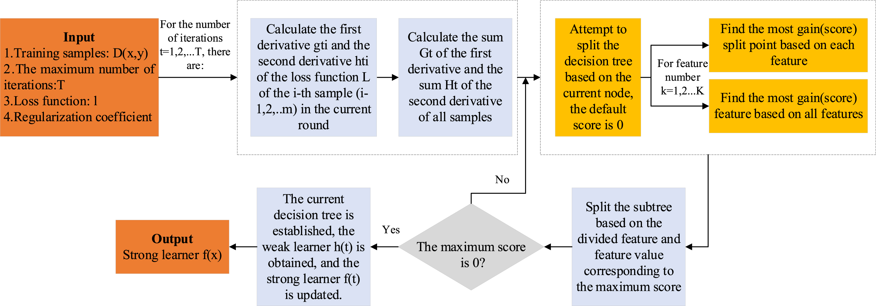
Optimal decision tree construction process.

Therefore, XGBoost model has two advantages over other traditional boosting tree models:

The objective function is approximated by a second-order Taylor expansion. The traditional gradient boosting decision tree model only uses the first derivative in the optimization. XGBoost performs the second-order Taylor expansion on the cost function and uses the first and second derivatives. The custom cost function is supported as long as the function satisfies the first and second order.

XGBoost defines the complexity of the tree. That is, XGBoost model adds a regular term to the cost function to control the complexity of the model and prevent over-fitting.

3 XGBoost prediction model implementation

3.1 Bicycle rental data preprocessing

Bike sharing systems are a means of renting bicycles where the process of obtaining membership, rental, and bike return is automated via a network of kiosk locations throughout a city. Using these systems, people are able rent a bike from a one location and return it to a different place on an as-needed basis. Currently, there are over 500 bike-sharing programs around the world. The data generated by these systems makes them attractive for researchers because the duration of travel, departure location, arrival location, and time elapsed is explicitly recorded. Bike sharing systems therefore function as a sensor network, which can be used for studying mobility in a city. This article combines historical usage patterns with weather data in order to forecast bike rental demand in the Capital Bike share program in Washington, D.C. Washington, D.C. is located in the Northeast and Mid-Atlantic regions of the United States, its specific location is shown in Fig. 3.

Fig. 3

USA Map with Capitals.

The raw data used in this article is hourly bicycle rental data recorded by the Washington, D.C. bicycle rental system during 2011 and 2012. The data set includes 10,886 observations for twelve variables. Table 1 shows some of the data in the original bicycle rental data.

Table 1

Example of bicycle rental data

datetime	season	holiday	workingday	weather	temp	atemp	humidity	windspeed	casual	registered	count
2011/1/1 0 : 00	1	0	0	1	9.84	14.395	81	0	3	13	16
2011/1/1 1 : 00	1	0	0	1	9.02	13.635	80	0	8	32	40
2011/1/1 2 : 00	1	0	0	1	9.02	13.635	80	0	5	27	32
2011/1/1 3 : 00	1	0	0	1	9.84	14.395	75	0	3	10	13

As can be seen from Table 1, there are a total of 12 columns of data. The definition of each data field is shown in Table 2.

Table 2

Data field explanation

Id	Feature	Range	Explain
1	datetime	/	Format: year/month/day hour
2	season	/	1: spring, 2: summer, 3: autumn, 4:winter
3	holiday	/	Whether it is a holiday,1:yes; 0:no
4	workingday	/	Whether it is a working day, 1: yes; 0: no
5	weather	/	1: Sunny weather or less clouds, 2: Foggy and clouds / wind 3: Light snow/light rain, lightning and cloudy, 4: Heavy rain / hail / lightning and heavy fog / heavy snow
6	temp	[0.82,41]	Celsius
7	atemp	[0.76,46)	The temperature people feel
8	humidity	0,100]	Humidity
9	windspeed	[0,57)	Wind speed
10	casual	0,367]	Number of unregistered people who book bicycles
11	registered	[0,886]	Number of registered people who book bicycles
12	count	[1,997]	Total bicycle demand = casual+registered (label)

This article selects the variables datetime, season, holiday, workingday, weather, temp, atemp, humidity, and windspeed for model training and then predicts the number of bicycle rentals. Since the datetime feature format is given in the form of “year/month/day.hour”, may be prompted for formatting errors during data reading. In order to unify the data format, this paper extracts year, month, day, and hour from the datetime feature. The datetime feature can be deleted, so the number of features used to train the model becomes 12, the results are shown in Table 3.

Table 3

Example of bicycle rental data after adding features

season	holiday	workingday	weather	temp	atemp	humidity	windspeed	year	month	day	hour	count
1	0	0	1	9.84	14.395	81	0	2011	1	1	0	16
1	0	0	1	9.02	13.635	80	0	2011	1	1	1	40
1	0	0	1	9.02	13.635	80	0	2011	1	1	2	32
1	0	0	1	9.84	14.395	75	0	2011	1	1	3	13
1	0	0	1	9.84	14.395	75	0	2011	1	1	4	1

3.2 Feature selection of bicycle rental demand data

Feature selection refers to transforming samples in high-dimensional space into low-dimensional space by means of mapping or transformation, which reduces dimensionality, and then further reducing dimensionality through feature selection of redundant and unrelated items [38]. The principle of feature selection is to obtain as small a feature subset as possible without significantly reducing the accuracy of estimation or affecting the data distribution. Feature selection methods are roughly divided into two types based on whether they use correlation coefficients or learning models. In this paper, the feature importance analysis method based on learning model is adopted. This method uses the machine learning algorithm to build a prediction model for each individual feature and response variable, which can better mine the relationship between features.

In this paper, the XGBoost model is used to analyze the importance of the feature. The advantage of this algorithm is that after the promotion tree is created, the importance score of each attribute can be directly obtained. The XGBoost model calculates the importance of the feature by summing the number of times the feature is split in each decision tree [39]. In a single decision tree, the closer an attribute is to the root node, the greater the weight; the more the tree is selected, the more important the attribute is. Finally, the results of an attribute for all of the boosting trees are averaged by weighted summation to obtain the order of feature importance. The principle of feature importance analysis of the XGBoost model is shown in Fig. 4.

Fig. 4

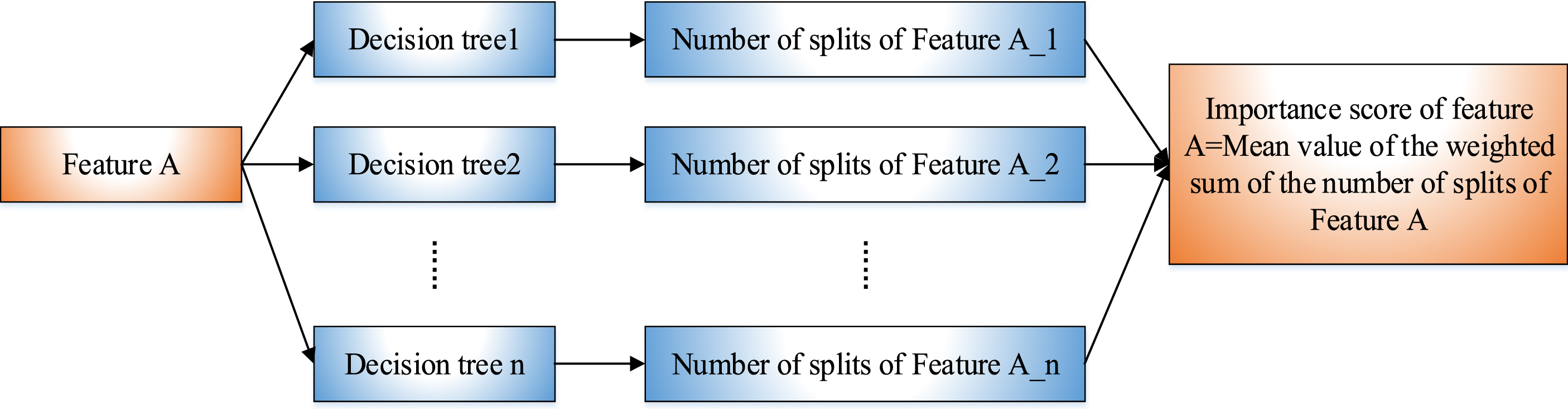
Feature Importance Analysis of XGBoost Model.

The 13 features – season, holiday, workingday, weather, temp, atemp, humidity, windspeed, year, month, day, hour, and count – are input into the XGBoost model for training, and the importance of the remaining 12 features except count is analyzed. Importance is defined as the extent to which each feature affects the count value to be predicted. The results of the feature importance analysis are shown in Fig. 5.

Fig. 5

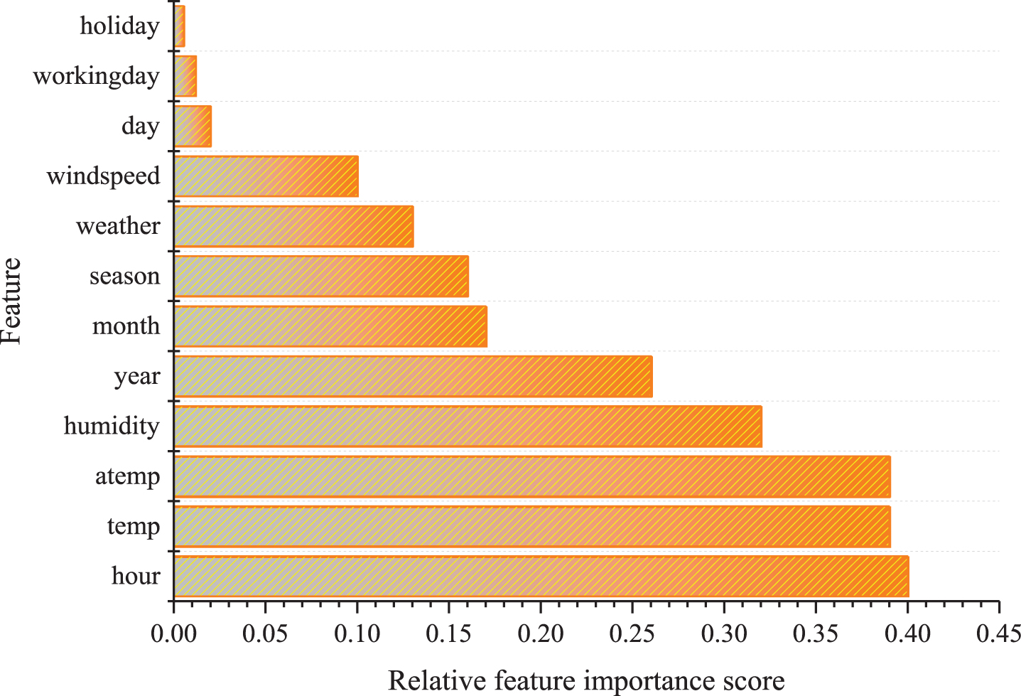
Feature Importance Analysis Based on XGBoost Model.

To demonstrate visually the correlations between the features and also between the features and the predicted count value, a thermal map of the matrix of feature correlation coefficients is presented in Fig. 6. The closer the absolute value of the correlation between a given feature and count is to 1, the more relevant the features are. A correlation coefficient of 0 indicates that the feature is irrelevant. The features with low importance, as shown in Figs. 5 and 6, are removed in the model training. According to the characteristic thermogram, for two or more features with strong correlation, only one of the features is retained for model training, in general, the absolute value of the correlation coefficient is greater than 0.8, and the two variables are considered to be strongly correlated. For example, the correlation coefficients of the features temp and atemp are as high as 0.98, so one of the features can be selected. Therefore, to ensure the stability and accuracy of the machine learning model, highly relevant features are deleted during the modeling process, which avoids the interaction between different features [40].

Fig. 6

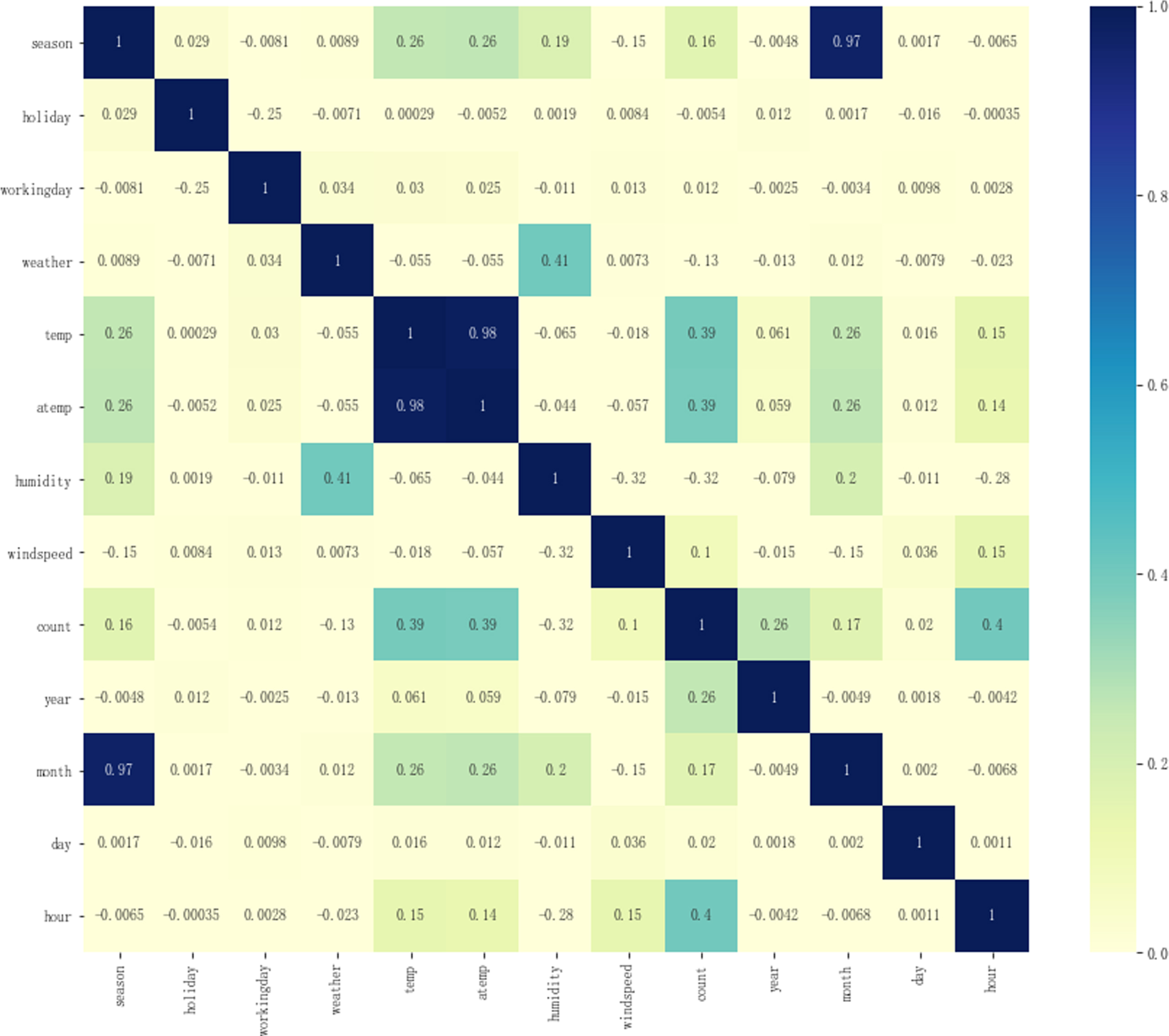
Thermal map of the matrix of feature correlation coefficients.

3.3 Optimized XGBoost prediction model based on a grid search algorithm

3.3.1 Grid Search principle

Parameter optimization is an effective method to improve the accuracy of prediction. Manually adjusting parameters is high complexity and labor-intensive and requires continuous testing. The grid search (GS) is a common parameter optimization method, it is easy to implement. The algorithm tried various parameter combinations to find the optimal parameters. GS has high parallelism [41]. Some of the common parameters of XGBoost are independent of each other, and some influence each other. The GS algorithm can meet this flexible characteristic. Therefore, this paper proposes a parameter optimization method for the XGBoost model based on a GS algorithm which automatically finds the optimal parameter value for the model. The GS algorithm is an exhaustive search method for specifying parameter values. The parameters of the estimation function are optimized using a cross-validation method to obtain an optimal learning algorithm. The algorithm arranges and combines all of the possible values of each parameter. With all of the parameters listed, the possible combined results generate a “grid,” and each parameter combination is used for model training while cross-validation is used to evaluate model performance.

In the process of actual parameter optimization, cross-validation and GS are combined as a model evaluation method referred to as “Grid Search with Cross Validation.” Cross-validation is used to divide the original data set randomly. The training set is divided into k subsets. Each training takes one subset as the verification set, and the remaining subsets are training sets. Therefore, k verification sets can be selected. This article uses 5-fold cross-validation to evaluate the results of the GS. Figure 7 shows the process of five-fold cross-validation, that is, 5 iterations of cross-validation are performed, and 5 model scores are obtained.

Fig. 7

5-fold cross-validation schematic.

3.3.2 Optimization of XGBoost model parameters based on grid search

In this paper, the GS algorithm is used to optimize the common parameters of the XGBoost model. Parameter optimization can improve the prediction accuracy of the model to some extent. The XGBoost model parameters are divided into general parameters, booster parameters, and task parameters. This paper optimizes the general parameters and booster parameters of the XGBoost model. The common parameters of the model and their meanings are shown in Table 4.

Table 4
Model parameters

Parameter

1 n_estimators

2 min_child_weight

3 max_depth

4 gamma

5 subsample

6 colsample_bytree

7 reg_alpha

8 reg_lambda

9 learning_rate

	Parameter
1	n_estimators
2	min_child_weight
3	max_depth
4	gamma
5	subsample
6	colsample_bytree
7	reg_alpha
8	reg_lambda
9	learning_rate

This paper will optimize the nine parameters in Table 4. This paper divides the training set and test set according to the ratio of 7 : 3. The cross-validation and grid search algorithm combined with the specific process of optimizing the XGBoost model parameters is shown in Fig. 8. The grid search optimizes model parameters six times, and nine model parameter values, including the n_estimators parameter, are optimized. Through continuous search and verification, a set of optimal parameter values will be obtained, and the prediction model will be re-established according to these values.

Fig. 8

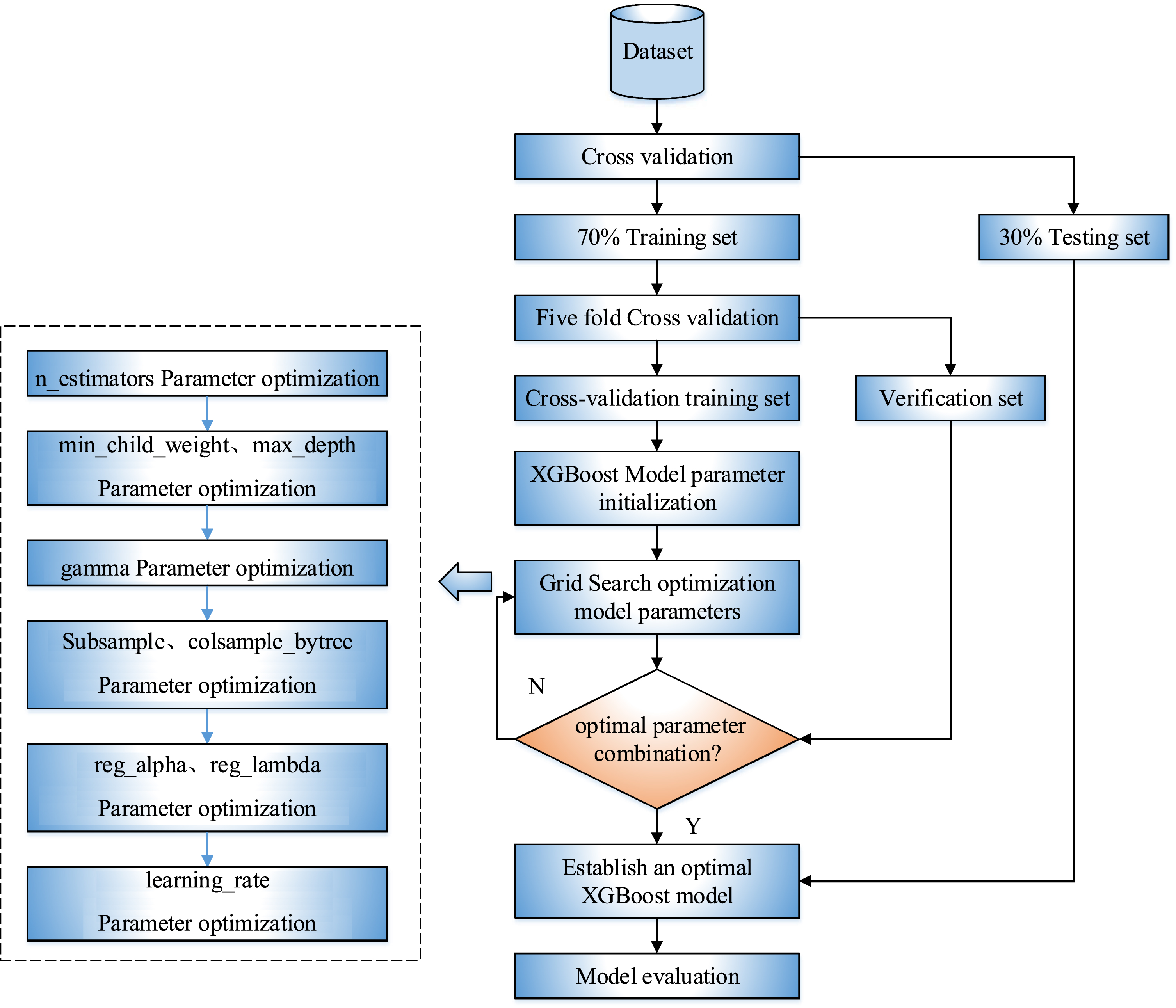
Flowchart for optimizing XGBoost model parameters.

1) Optimizing the n_estimators parameter

This paper first optimizes the n_estimators parameter. The search range is 550–675, and the step size is 25. The comparison of the model scores corresponding to different n_estimators values is shown in Fig. 9a. It can be seen that when n_estimators = 675, the performance of the model is the strongest.

Fig. 9

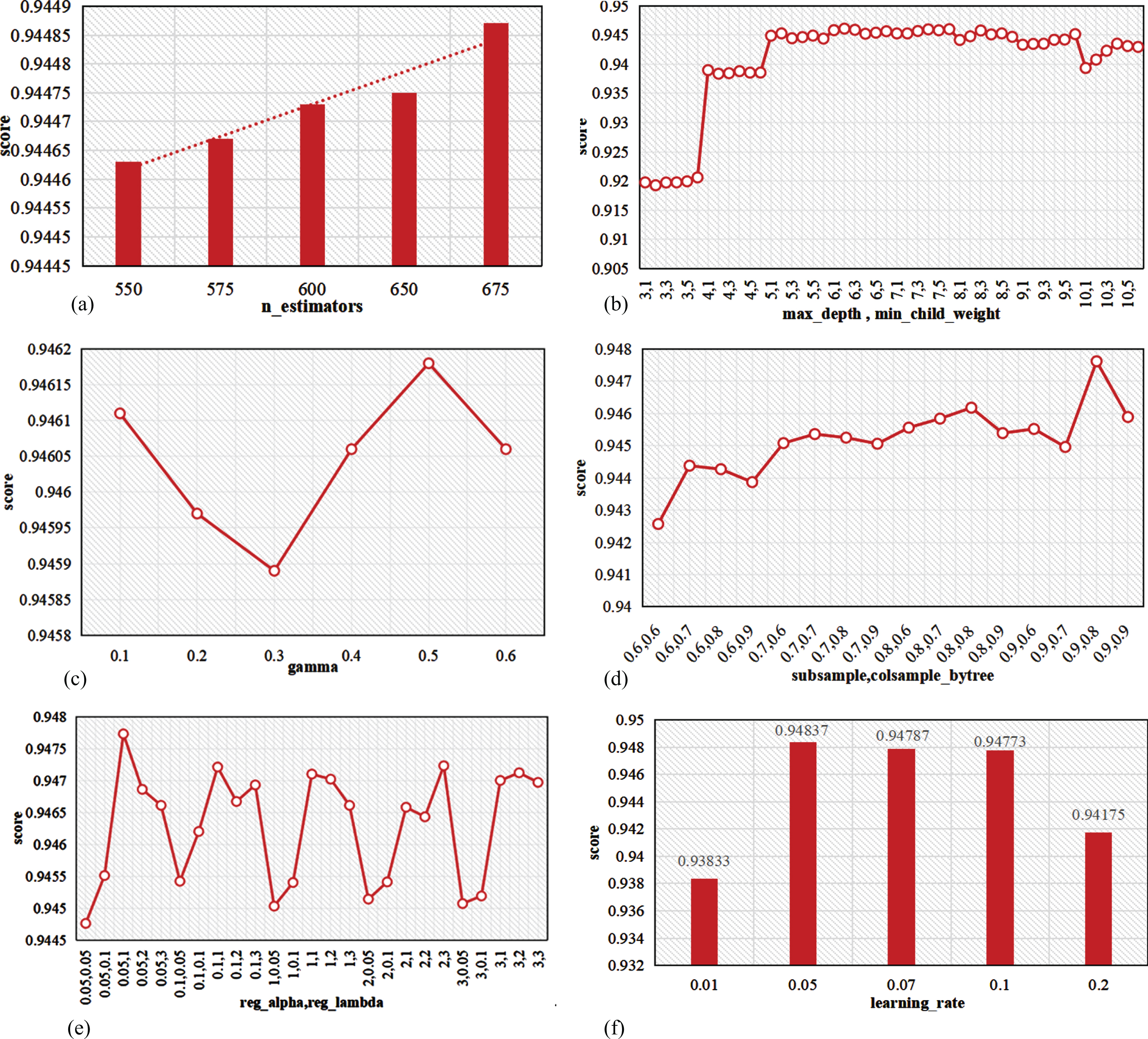
Model parameter optimization. a) n_estimators. b) max_depth and min_child_weight. c) gamma. d) subsample and colsample_bytree. e) reg_alpha and reg_lambda. f) learning_rate.

2) Optimizing the min_child_weight and max_depth parameters

Setting the n_estimators value to the optimal value of 675 during the second grid search, the remaining parameter values are initially their default values. To search for the best value of max_depth in the range of 3–10, the step size is set to 1. To search for the best value of min_child_weight in the range of 1–6, the step size is set to 1. The model scores under different parameter values are shown in Fig. 9b. It can be seen that the model prediction effect is best when max_depth = 6 and min_child_weight = 2.

3) Optimizing the gamma parameters

When performing the third grid search, the n_estimators value is set to the optimal value 675. The max_depth and min_child_weight parameters are set to the optimal values of 6 and 2, respectively. The remaining parameters are initially set to their default values. The model scores under different gamma parameters are shown in Fig. 9c. The model score is highest when gamma = 0.5.

4) Optimizing the subsample and colsample_bytree parameters

In the fourth grid search, the n_estimators value is set to the optimal value of 675. The max_depth and min_child_weight parameter values are set to 6 and 2, respectively. The gamma parameter value is set to 0.5. The remaining parameters are initially set at their default values. The search range for the subsample and colsample_bytree parameters is 0.6–0.9 with a step size of 0.1. The results are shown in Fig. 9d. The model prediction is best when subsample = 0.9 and colsample_bytree = 0.8.

5) Optimize the reg_alpha and reg_lambda parameter

In the fifth grid search, the n_estimators value is set to the optimal value of 675. The max_depth and min_child_weight are set to the optimal values of 6 and 2, respectively. The gamma parameter value is set to the optimal value of 0.5. The subsample and colsample_bytree are set to 0.9 and 0.8, respectively. The remaining parameters are initially set at their default values. The search ranges are 0.05–0.1 for reg_alpha and 1–3 for reg_lambda. The model scores under different parameter values are shown in Fig. 9e. The model prediction is best when reg_alpha = 0.05 and reg_lambda = 1.

6) Optimize the learning_rate parameter

In the sixth grid search, the n_estimators value is set to the optimal value of 675. The max_depth and min_child_weight are set to the optimal values of 6 and 2, respectively. The gamma parameter value is set to the optimal value of 0.5. The subsample and colsample_bytree are set to 0.9 and 0.8, respectively. The reg_alpha and reg_lambda parameters are set to the optimal values of 0.05 and 0.1, respectively. The remaining parameters are initially set at their default values. The search range for the optimal value of the learning_rate parameter is the following set of values: 0.01, 0.05, 0.07, 0.1, and 0.2. The model scores under different parameter values are shown in Fig. 9f. The model prediction is best when learning_rate = 0.05.

After the grid search is adjusted, the optimal parameters of a set of XGBoost models are obtained, as shown in Table 5. The bicycle rental demand forecasting model is established according to the optimal parameters, and the regression model evaluation index is used to analyze model fit before and after optimization.

Table 5

Optimal parameter combination

	Optimal parameter value
1	n_estimators=675
2	min_child_weight=2
3	max_depth=6
4	gamma=0.5
5	Subsample=0.9
6	colsample_bytree=0.8
7	reg_alpha=0.05
8	reg_lambda=0.1
9	learning_rate=0.05

3.4 Evaluation indicators of regression prediction model

The regression model generally uses the indicators of Mean Absolute Error (MAE), Mean Squared Error (MSE), and R-squared to evaluate and analyze the prediction results, as shown in Table 6.

Table 6
Evaluation index

Evaluation index Description

1 Mean Absolute Error(MAE) Average absolute error

2 Mean Square Error(MSE) Mean square error

3 Root Mean Squard Error(RMSE) Root mean square error

4 R-Squared R squared value

	Evaluation index	Description
1	Mean Absolute Error(MAE)	Average absolute error
2	Mean Square Error(MSE)	Mean square error
3	Root Mean Squard Error(RMSE)	Root mean square error
4	R-Squared	R squared value

In addition to the regression model evaluation indicators commonly found in Table 6, this paper uses a new evaluation index Root Mean Squared Logarithmic Error, it is expressed as: $RMSE = \sqrt{\frac{\sum_{i = 1}^{n} (y_{i} - {\hat{y}}_{i})^{2}}{n}}$ (17)

The root mean squared logarithmic error is expressed as: $RMSLE = \sqrt{\frac{1}{n} \sum_{i = 1}^{n} {(log (y_{i} + 1) - log ({\hat{y}}_{i} + 1))}^{2}}$ (18)

Where n is the number of samples, y_i is the true value, and ${\hat{y}}_{i}$ is the predicted value. The smaller the root mean square logarithmic error, the better the fit of the model.

4. Analysis of forecast results of bicycle rental demand

4.1 Comparison of the prediction results of the XGBoost model before and after optimization

Following to the feature selection principle, 6 features (season, weather, temp, humidity, windspeed, and hour) are used as input variables to construct the XGBoost bicycle rental demand forecasting model. Figure 10 is a comparison of the results of bicycle demand forecast before and after optimization of the XGBoost model. Figure 10a is a comparison of the predicted values of rental count from XGBoost model before optimization and the observed values. Figure 10c is a comparison of the predicted values from an XGBoost model based on the grid search algorithm and the observed values. Figure 10c is a comparison of the difference between the predicted and observed values of rental count for the model before and after optimization. Figure 11 shows the fitting effect of the real and predicted values of the model before and after optimization. According to Figs. 10 and 11, the optimized XGBoost model fits the data better than the regular XGBoost model and more accurately predicts changes in bicycle demand. The error between the optimized model prediction value and the real value is significantly reduced, thereby more accurately predicting the bicycle rental demand.

Fig. 10

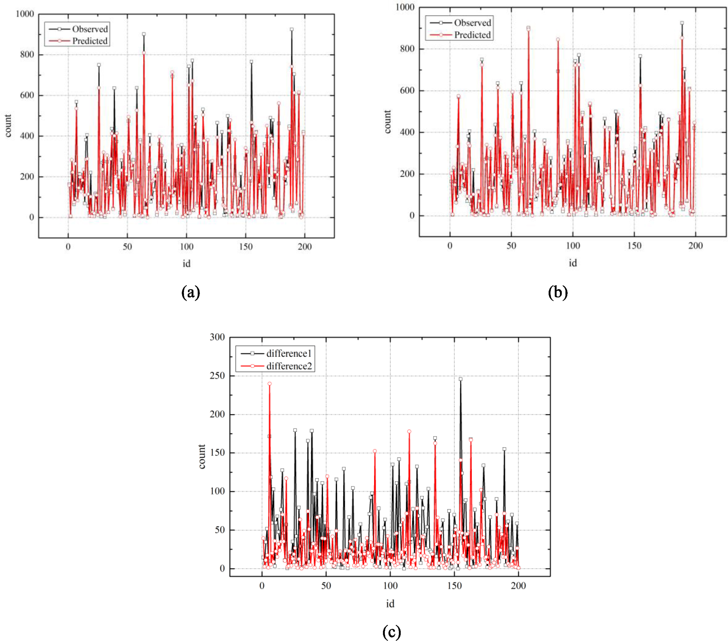
Comparison of XGBoost model and optimized XGBoost model prediction. (difference1 indicates the absolute value of the difference between the predicted value of the XGBoost model and the observed value, difference2 indicates the absolute value of the difference between the predicted value of the optimized XGBoost model based on the grid search algorithm and the observed value.) a) The prediction results of the XGBoost model. b) The prediction results of the optimized XGBoost model. c) The absolute value of difference between observed values and predicted values.

Fig. 11

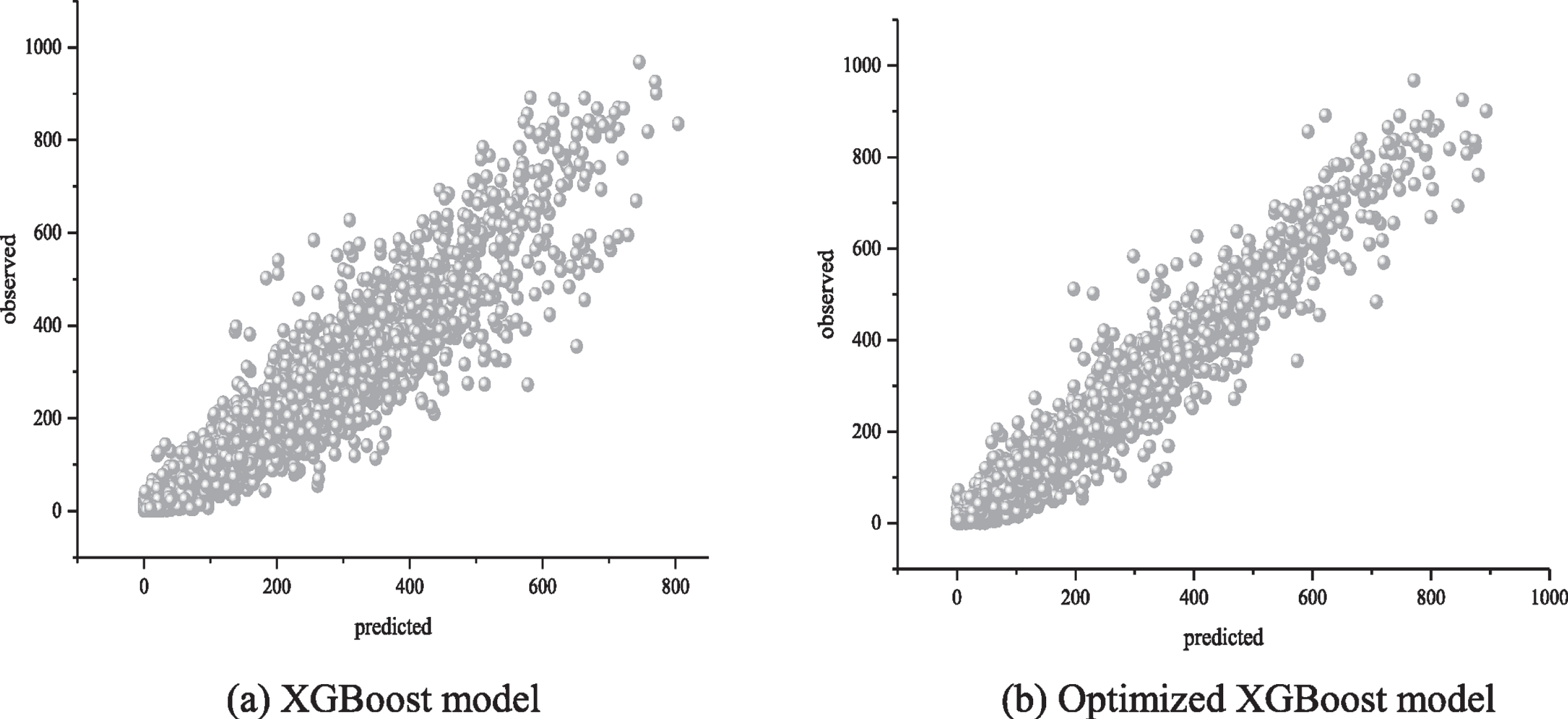
Fitting effect of the observed value and predicted value of bicycle demand.

This paper uses RMSLE, MAE, R-Squared, and the Pearson correlation coefficient to measure the performance of the XGBoost model before and after optimization. Table 7 analyzes the performance of the XGBoost model and the optimized XGBoost model by taking the 2012 data in the test set as an example, and analysis of model evaluation index values of three characteristics of season, workingday and temp. Table 8 takes the entire test set as an example to compare and analyze the performance of the model before and after optimization.

Table 7

Comparison of model evaluation indicators in different seasons, on working or weekend days, and for different temperatures

		XGBoost				Optimized XGBoost model
		RMSLE	MAE	R-Squared	Pearson	RMSLE	MAE	R-Squared	Pearson
Season	spring	0.599	35.76	0.878	0.937	0.592	24.94	0.939	0.969
	summer	0.518	57.96	0.876	0.936	0.507	38.34	0.943	0.971
	autumn	0.514	55.57	0.883	0.940	0.474	42.10	0.931	0.964
	winter	0.478	49.60	0.875	0.935	0.471	34.90	0.940	0.969
Working day	no	0.522	50.04	0.876	0.936	0.537	39.85	0.923	0.961
	yes	0.536	48.96	0.892	0.944	0.506	32.53	0.950	0.974
Temp	0–10	0.666	30.95	0.839	0.916	0.570	15.14	0.937	0.968
	10–20	0.579	42.48	0.865	0.930	0.528	23.87	0.942	0.970
	20–30	0.514	56.23	0.885	0.941	0.505	34.52	0.937	0.968
	30–40	0.241	62.08	0.814	0.902	0.163	38.36	0.910	0.954

Table 8

Comparison of model evaluation indicators before and after optimization

Model	RMSLE	MAE	R-Squared	Pearson
XGBoost Model	0.552	43.81	0.879	0.938
Optimized XGBoost Model	0.495	28.481	0.947	0.973

Tables 7, 8 illustrate the effectiveness of the grid search algorithm. Smaller RMSLE and MAE values indicate smaller differences between the predicted and observed values of the dependent variable. Larger R-Squared and Pearson correlation coefficients indicate better model fit for the data. Compared to the regular XGBoost model, the XGBoost model using grid search optimization can better describe the variation of the original data. Finding the optimal combination of parameters improves the accuracy of the XGBoost model in predicting hourly bicycle. The optimized model can better explore the changing trend of Washington, D.C. bicycle demand and provide information that will help promote the development of the city’s public bicycle rental system.

4.2 Comparison of prediction results of different models

Different regression algorithms will produce different effects under the same data conditions. Therefore, this paper compares the XGBoost algorithm with the classic SVM and RF algorithm. Similarly, three indicators, RMSLE, MAE, and R-Squared, are used to evaluate the performance of different models. The prediction accuracy of different kernel functions of the support vector machine is analyzed through experiments, and it is found that the prediction error of linear kernel and Gauss radial basis function are small under the same data conditions, and the performance of the linear kernel is better than the Gauss radial basis function.

C and gamma are crucial parameters in SVM, and these two parameters are independent of each other [42]. The parallelism of the GS algorithm is very suitable for optimizing the parameters of the SVM. After parameter optimization by the GS algorithm, the support vector machine regression prediction result is more accurate under the condition that the kernel function is the Gauss radial basis function. Similarly, the grid search algorithm is used to optimize the parameters of the RF, and the specific parameter optimization results are shown in Table 9.

Table 9
Parameter settings of support vector machine and random forest

SVM Random forest

C = 1000 max_depth = 36

epsilon = 0.1 min_samples_split = 2

gamma = 0.01 min_samples_leaf = 1

kernel = ’rbf ’ n_estimators = 710

max_features = 12

SVM	Random forest
C = 1000	max_depth = 36
epsilon = 0.1	min_samples_split = 2
gamma = 0.01	min_samples_leaf = 1
kernel = ’rbf ’	n_estimators = 710
	max_features = 12

The comparison results of the evaluation indexes of the three models after the GS optimization parameters are shown in Fig. 12. It can be seen that the optimized XGBoost model has the highest prediction accuracy and the smallest prediction error; random forest comes next; SVM have the worst performance. Compared with other algorithms, XGBoost reduces the error generated during model training by adding a regular term to the objective function. At the same time, the algorithm performance improves the prediction accuracy to a certain extent. This shows that the XGBoost algorithm maintains a strong generalization ability and stability in regression prediction examples, and can provide more reliable data information.

Fig. 12

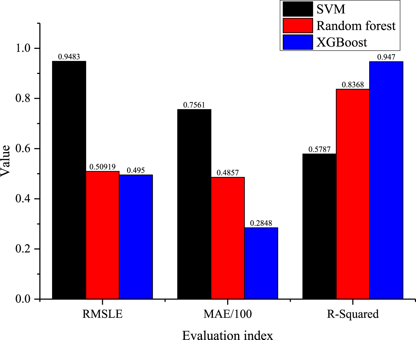
Evaluation results of different models.

This paper analyzes how bicycle demand across seasons, months, hours of the day, and different temperatures. Taking part of the data of 2012 in the test set as an example, Fig. 13 shows the accumulated bicycle demand in different seasons, different months and different time points in 2012.

Fig. 13

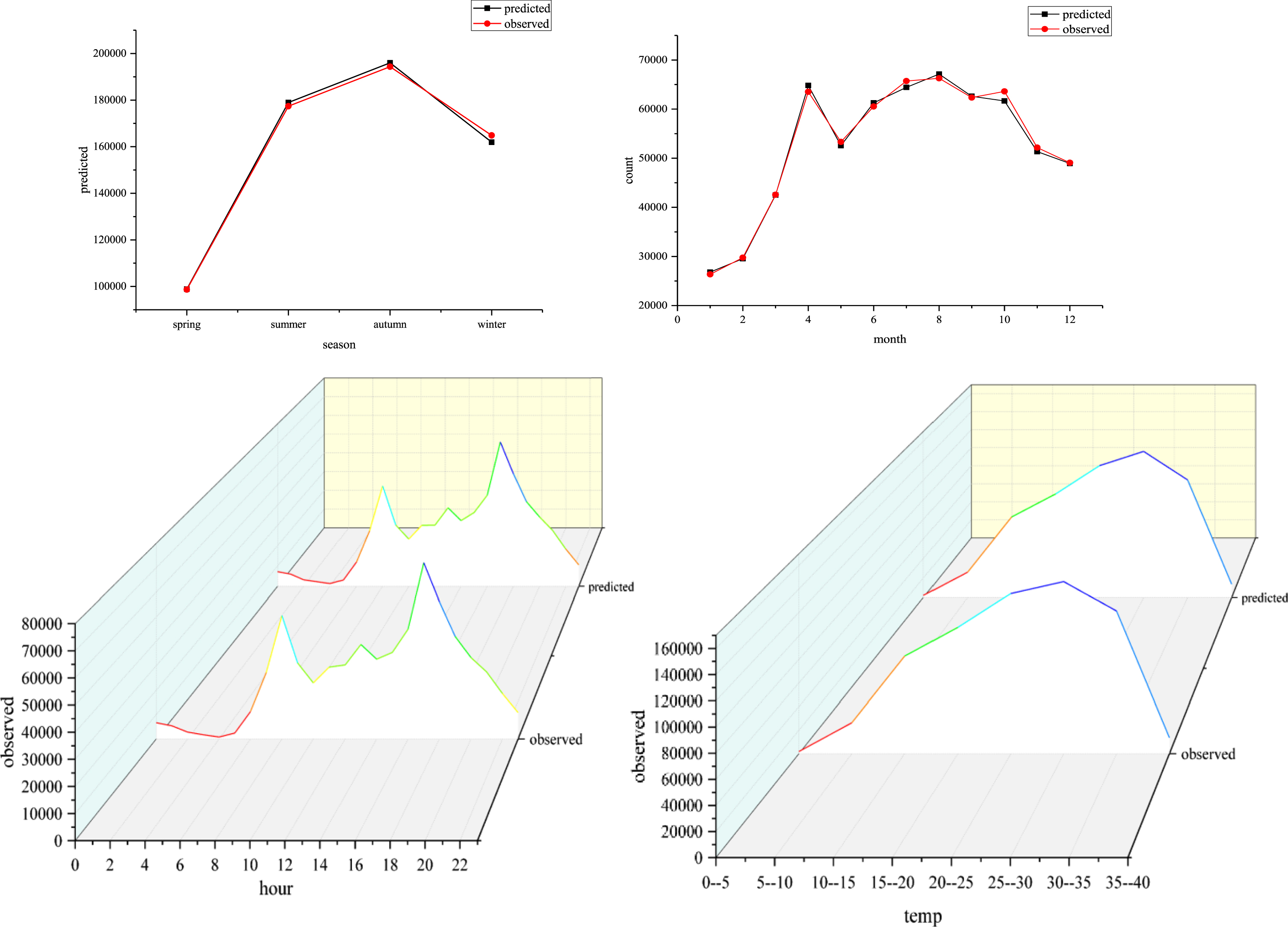
Analysis of bicycle demand in different seasons, different months, different times and different temperatures.

Analysis of Fig. 13 leads to the following conclusions:

The demand for bicycles is relatively large from April to October every year, and it is growing rapidly in March-April. The relevant management departments of Washington, D.C. can increase the amount of bicycles during this period.

The daily demand for bicycles sharply increases from 7am to 9am and 4pm to 8pm is increasing rapidly. These two periods are the morning peak and the evening peak, respectively. During these periods, more public bicycles can be made available to avoid shortages during peak hours. According to the changes in bicycle demand across different time periods, the amount of bicycles can be reasonably arranged, which can effectively alleviate the urban traffic pressure during the peak period.

Weather factors also have a significant influence on the number of bicycles demand. When the temperature is between 15–35 degrees, the number of bicycles rented is large.

5 Conclusion and future wok

To solve the problems of unanticipated bicycle rentals and imbalances of supply and demand in the management process of the public bicycle system, this paper proposes a bicycle demand forecasting model based on GS and XGBoost fusion model. Bicycle rental data provided by the Washington City Bicycle Rental System is used to verify the performance of the proposed model. Through discussion and analysis, the following points can be drawn:

This paper used the tree model-based method to analyze the importance of the features of season, holiday, workingday, weather, temp, atemp, humidity, windspeed, year, month, day, and hour. This method reveals potentially non-linear relationships between features. The results show that hour, atemp,temp and humidity factors are strongly correlated with changes in bicycle demand. At the same time, there is a strong correlation between temp and atemp,to avoid the interaction between features, atemp is deleted.To ensure the stability and accuracy of the model, the features that have low correlation with the target value are deleted.

This paper constructs a bicycle demand forecasting model based on GS and XGBoost. Through the GS algorithm, the nine commonly used parameters of the prediction model are tuned, and then the optimized parameters are used to re-establish the prediction model. improving prediction accuracy. Comparing XGBoost model, optimized XGBoost has higher prediction accuracy, R-Squared is 0.947.This method overcomes the instability of traditional neural network algorithms, has strong generalization ability, and shows excellent performance when processing massive data.

This paper uses the GS algorithm to optimize the important parameters of the SVM and the RF model, and compares the model proposed in this paper with these models. The results show that the predicted value of the optimized XGBoost model is closer to the true value. This method solves the problem of low prediction accuracy of traditional algorithms.

The research work of this paper can provide data support for the efficient distribution of public bicycles and provide a theoretical basis for the effective development of the city’s public bicycle management system and the full use of public resources. Further, the paper explores trends in bicycle demand more comprehensively and demonstrates that future research should integrate predictive models with other models. This will improve generalization ability and generate more accurate predictions of bicycle demand, making the development of urban public transportation system more scientific and rational.

Footnotes

Acknowledgments

The author sincerely thanks the Prof. Z.S. and Prof. W.L. for her help and coaching. At the same time, the authors would like to express thanks to the anonymous reviewers for providing valuable comments.

Funding details

This paper is based on the research conducted by the National Key Research and Development Program, China (Grant number: 2018YFB1600202), with help of Prof. Z.S.; the National Natural Science Foundation of China (Grant number: 51978071), with help of Prof. W.L.

Data availability statement

Some or all data, models, or code generated or used during the study are available from the Second author by request.

Competing interests

The authors declare that they have no competing interests.

References

mzwagerman, Bike-share systems: accessibility and availability, (2015).

Shui

C.S.

and Szeto

W.Y.

, A review of bicycle-sharing service planning problems, Transportation Research Part C Emerging Technologies 117 (2020), 102648.

Oskarbski

, Birr

and Zarski

, Bicycle Traffic Model for Sustainable Urban Mobility Planning, Energies 14(18) (2021).

Shen

, Wei

, Sun

, Rao

K.S.

and Wang

, A Hybrid Dispatch Strategy Based on the Demand Prediction of Shared Bicycles, Applied Sciences 10(8) (2020), 2778. doi:10.3390/app10082778.

Kaltenbrunner

, Meza

, Grivolla

, Codina

and Banchs

, Urban cycles and mobility patterns: exploring and predicting trends in a bicycle-based public transport system, Pervasive and Mobile Computing 6(4) (2010), 455–466.

Borgnat

, Robardet

, Abry

, Flandrin

, Rouquier

J.B.

and Tremblay

, A dynamical network view of lyon’s vélo’v shared bicycle system, (2013).

Vogel

, Greiser

and Mattfeld

D.C.

, Understanding bike-sharing systems using data mining: exploring activity patterns, Procedia – Social and Behavioral Sciences 20(none) (2011), 514–523.

Vogel

and Mattfeld

D.C.

, Strategic and Operational Planning of Bike-Sharing Systems by Data Mining – A Case Study, International Conference on Computational Logistics, Springer, Berlin, Heidelberg, (2011).

Kuang

, Xu

and Lu

, Self-balanced bicycle rental systems under dynamic demand forecasting, International Conference on Fuzzy Systems & Knowledge Discovery, IEEE, (2014).

10.

Cantelmo

, Kucharski

and Antoniou

, Low-dimensional model for bike-sharing demand forecasting that explicitly accounts for weather data, Transportation Research Record Journal of the Transportation Research Board 2674(1) (2020), 036119812093216.

11.

Barnes

and Krizek

, Estimating bicycling demand, Transportation Research Record 1939 (2005), 45–51.

12.

Singhvi

, Singhvi

, Frazier

P.I.

, Henderson

S.G.

, Mahony

E.O.

, Shmoys

D.B.

, et al., Predicting Bike Usage for New York City’s Bike Sharing System, (2015).

13.

Yajun

, Lilei

, Rong

and Yulong

, A markov chain based demand prediction model for stations in bike sharing systems, Mathematical Problems in Engineering 2018 (2018), 1–8.

14.

Zhang

, Xiao

, Li

and Yu

P.S.

, Bicycle-sharing system analysis and trip prediction, IEEE, (2016).

15.

Febres

J.D.

, Mohamadi

and Mariscal

M.A.

, The Role of Journey Purpose in Road Traffic Injuries: A Bayesian Network Approach, Journal of Advanced Transportation, (2019).

16.

Fournier

, Christofa

and Knodler

M.A.

, A sinusoidal model for seasonal bicycle demand estimation, Transportation Research Part D Transport & Environment 50(JAN.) (2017), 154–169.

17.

Zhang

, Zhou

, Hao

and Zhou

, Prediction model of demand for public bicycle rental based on land use, Advances in Mechanical Engineering 10(12) (2018), 168781401881897.

18.

Ryu

, Su

, Chen

and Choi

, Estimating bicycle demand of a small community, Ksce Journal of Civil Engineering 23(6) (2019), 2690–2701.

19.

and Gpg

, Random parameter models for estimating statewide daily bicycle counts using crowdsourced data sciencedirect, Transportation Research Part D: Transport and Environment, 84.

20.

Chibwe

, Heydari

, Imani

A.F.

and Scurtu

, An exploratory analysis of the trend in the demand for the bike-sharing system: from london olympics to covid-19 pandemic, Sustainable Cities and Society 69(3) (2021), 102871.

21.

Martins Dias

, Bellalta

and Oechsner

, Predicting occupancy trends in barcelona’s bicycle service stations using open data, (2015).

22.

Chen

, Jiang

Y.K.

and Li

M.Y.

, Research on Single-station Scheduling Demand of Public Bicycle Based on BP Neural Network, Journal of Transportation Research 3 (2016), 30–35.

23.

Feng

Y.L.

and Wang

S.S.

, A forecast for bicycle rental demand based on random forests and multiple linear regression, 2017 IEEE/ACIS 16th International Conference on Computer and Information Science (ICIS), IEEE, (2017).

24.

Kang

, Zuo

, Huang

, Zhou

and Chen

, Research on the Forecast of Shared Bicycle Rental Demand Based on Spark Machine Learning Framework, 2017 16th International Symposium on Distributed Computing and Applications to Business, Engineering and Science (DCABES), IEEE Computer Society, (2017).

25.

Yao

, Shen

, He

and Son

S.H.

, Demand Estimation of Public Bike-Sharing System Based on Temporal and Spatial Correlation, 2018 4th International Conference on Big Data Computing and Communications (BIGCOM), IEEE Computer Society, (2018).

26.

Gao

and Lee

G.M.

, Moment-based rental prediction for bicycle-sharing transportation systems using a hybrid genetic algorithm and machine learning, Computers & Industrial Engineering 128 (2019), 60–69.

27.

, Li

, Gan

, Zhang

, Yu

, Chen

, et al., A deep learning approach on short-term spatiotemporal distribution forecasting of dockless bike-sharing system, Neural Computing and Applications, (2018).

28.

, Duan

and Pu

, Dynamic bicycle scheduling problem based on short-term demand prediction, Applied Intelligence, (2018).

29.

Chen

P.C.

, Hsieh

H.Y.

, Sigalingging

X.K.

, Chen

Y.R.

and Leu

J.S.

, Prediction of Station Level Demand in a Bike Sharing System Using Recurrent Neural Networks, IET Intelligent Transport Systems 14(6) (2020), 556–561.

30.

Seo

Y.H.

, Yoon

, Kim

D.K.

, Kho

S.Y.

and Hwang

, Predicting demand for a bike-sharing system with station activity based on random forest, Municipal Engineer 174(2) (2020), 1–24.

31.

, Lin

, Gao

, Meng

and Song

, Short-term rental forecast of urban public bicycle based on the hosvd-lstm model in smart city, Sensors (Basel, Switzerland) 20(11) (2020).

32.

, Hong

, Zhao

, Wang

and Zheng

, Neural networks with improved extreme learning machine for demand prediction of bike-sharing, Mobile Networks and Applications (Jan) (2021).

33.

Hastie

, Tibshirani

and Friedman

, Ensemble Learning, Springer, New York, (2009).

34.

Chen

, Tong

and Benesty

, Xgboost: extreme gradient boosting, (2016).

35.

Zounemat-Kermnai

, Batelaan

, Fadaee

and Hinkelmann

, Ensemble machine learning paradigms in hydrology: a review, Journal of Hydrology (2021), 126266.

36.

Nie

, Roccotelli

, Fanti

M.P.

, Ming

and Li

, Prediction of home energy consumption based on gradient boosting regression tree, Energy Reports 7(7) (2021), 1246–1255.

37.

Mitchell

, Adinets

, Rao

and Frank

, Xgboost: scalable gpu accelerated learning, (2018).

38.

Thirumoorthy

and Muneeswaran

, Feature selection for text classification using machine learning approaches, National Academy Science Letters (2021), 1–6.

39.

Singh

, Nagar

, Sharma

and Kotiyal

, A Gaussian process regression approach to predict the k-barrier coverage probability for intrusion detection in wireless sensor networks, Expert Systems with Applications 172 (2021), 114603.

40.

Tolosi

and Lengauer

, Classification with correlated features: unreliability of feature ranking and solutions, Bioinformatics 27(14) (2011), 1986–1994.

41.

Sun

, Ding

, Zhang

and Jia

, An improved grid search algorithm to optimize svr for prediction, Soft Computing (10) (2021).

42.

Singh

, Kotiyal

, Sharma

, Nagar

and Lee

C.C.

, A machine learning approach to predict the average localization error with applications to wireless sensor networks, IEEE Access 8 (2020), 208253–208263.

Forecasting public bicycle rental demand using an optimized eXtreme Gradient Boosting model

Abstract

Keywords

1 Introduction

2 XGBoost model construction principle

2.1 Principle of Boosting tree algorithm

3.1 Bicycle rental data preprocessing

3.3.1 Grid Search principle

Table 4 Model parameters Parameter 1 n_estimators 2 min_child_weight 3 max_depth 4 gamma 5 subsample 6 colsample_bytree 7 reg_alpha 8 reg_lambda 9 learning_rate

Table 6 Evaluation index Evaluation index Description 1 Mean Absolute Error(MAE) Average absolute error 2 Mean Square Error(MSE) Mean square error 3 Root Mean Squard Error(RMSE) Root mean square error 4 R-Squared R squared value

4.1 Comparison of the prediction results of the XGBoost model before and after optimization

Table 9 Parameter settings of support vector machine and random forest SVM Random forest C = 1000 max_depth = 36 epsilon = 0.1 min_samples_split = 2 gamma = 0.01 min_samples_leaf = 1 kernel = ’rbf ’ n_estimators = 710 max_features = 12

Footnotes

Acknowledgments

Funding details

Data availability statement

Competing interests

References

Table 4
Model parameters

Parameter

1 n_estimators

2 min_child_weight

3 max_depth

4 gamma

5 subsample

6 colsample_bytree

7 reg_alpha

8 reg_lambda

9 learning_rate

Table 6
Evaluation index

Evaluation index Description

1 Mean Absolute Error(MAE) Average absolute error

2 Mean Square Error(MSE) Mean square error

3 Root Mean Squard Error(RMSE) Root mean square error

4 R-Squared R squared value

Table 9
Parameter settings of support vector machine and random forest

SVM Random forest

C = 1000 max_depth = 36

epsilon = 0.1 min_samples_split = 2

gamma = 0.01 min_samples_leaf = 1

kernel = ’rbf ’ n_estimators = 710

max_features = 12